| Issue |
A&A
Volume 549, January 2013
|
|
|---|---|---|
| Article Number | A51 | |
| Number of page(s) | 8 | |
| Section | Extragalactic astronomy | |
| DOI | https://doi.org/10.1051/0004-6361/201219746 | |
| Published online | 18 December 2012 | |
NGC 6240: extended CO structures and their association with shocked gas⋆
1
IRAM – Institut de RadioAstronomie Millimétrique, 300 rue de la Piscine,
Domaine Universitaire,
38406
Saint Martin d’Hères,
France
e-mail: feruglio@iram.fr
2
INAF – Osservatorio astronomico di Roma, via Frascati
33, 00040
Monteporzio Catone,
Italy
3
Cavendish Laboratory, University of Cambridge,
19 J. J. Thomson Ave.,
Cambridge
CB3 0HE,
UK
4
XMM-Newton Science Operations Centre, ESAC, PO Box 78, 28691
Villanueva de la Canãda, Madrid, Spain
5
Laboratoire AIM-Paris-Saclay, CEA/DSM/Irfu, CNRS, Université Paris
Diderot, Saclay, pt courrier
131, 91191
Gif-sur-Yvette,
France
6
Max-Planck-Institut fur Extraterrestrische Physik
(MPE), Giessenbachstr.
1, 85748
Garching,
Germany
Received: 4 June 2012
Accepted: 5 November 2012
We present deep CO(1–0) observations of NGC 6240 performed with the IRAM Plateau de Bure Interferometer (PdBI). NGC 6240 is the prototypical example of a major galaxy merger in progress, caught at an early stage, with an extended, strongly-disturbed butterfly-like morphology and a heavily obscured active nucleus in the core of each progenitor galaxy. The CO line shows a skewed profile with very broad and asymmetric wings detected out to velocities of −600 km s-1 and +800 km s-1 with respect to the systemic velocity. The PdBI maps reveal two prominent structures of blueshifted CO emission. One extends eastward, i.e. approximately perpendicular to the line connecting the galactic nuclei, on scales of ~7 kpc, and it shows velocities up to −400 km s-1. The other extends southwestward out to ~7 kpc from the nuclear region, and has a velocity of −100 km s-1 with respect to the systemic one. Interestingly, redshifted emission with velocities 400 to 800 km s-1 is detected around the two nuclei, extending in the east-west direction, and partly overlapping with the eastern blueshifted structure, although tracing a more compact region of size ~1.7 kpc. The overlap between the southwestern CO blob and the dust lanes seen in HST images, which are interpreted as tidal tails, indicates that the molecular gas is deeply affected by galaxy interactions. The eastern blueshifted CO emission is cospatial with an Hα filament that is associated with strong H2 and soft X-ray emission. The analysis of Chandra X-ray data provides strong evidence of shocked gas at the position of the Hα emission. Its association with outflowing molecular gas supports a scenario where the molecular gas is compressed into a shock wave that propagates eastward from the nuclei. If this is an outflow, the active galactic nuclei are very likely the driving force.
Key words: galaxies: active / galaxies: interactions / galaxies: evolution / galaxies: ISM / quasars: general
© ESO, 2012
1. Introduction
The observed transformation of gas-rich star-forming galaxies into red, bulge-dominated spheroids devoid of gas is due to several mechanisms. In massive galaxies star formation might lead to a faster gas consumption rate than in less massive ones (Daddi et al. 2007; Peng et al. 2010; Elbaz et al. 2011; Rodighiero et al. 2011). In addition, galaxy interactions, mergers (Sanders et al. 1988; Barnes & Hernquist 1996; Cavaliere & Vittorini 2000; Di Matteo et al. 2005), together with active galactic nuclei (AGN) and starburst feedback, are expected to play a role (Silk & Rees 1998; King 2010, and references therein). Mergers can destabilize cold gas and trigger both star formation and nuclear accretion onto super-massive black holes (SMBHs), inducing AGN activity. A natural expectation of this scenario is that the early, powerful AGN phase is highly obscured by large columns of gas and dust (e.g. Fabian 1999). Once an SMBH reaches masses >107−8 M⊙, the AGN can efficiently contribute to the radiative heating of the interstellar medium (ISM) through winds and shocks, thus inhibiting further accretion and also star formation in the nuclear region and possibly on larger scales in the galactic disk. The radiative feedback from a luminous AGN is therefore a mechanism that could explain the low gas content of local massive galaxies and the galaxy bimodal color distribution (Kauffmann et al. 2003; Croton et al. 2006; Menci et al. 2006). This evolutionary scenario needs to be observationally confirmed. This can be achieved by observing systems during a major interaction phase. They probe both AGN and starburst-driven winds, and their interaction with the molecular gas. This represents the bulk of the gas in a galaxy.
Only recently have molecular gas outflows been discovered both in star-forming galaxies (e.g. M 82, Walter et al. 2002; Arp 220; Sakamoto et al. 2009) and in the hosts of powerful AGN, through the detection of both molecular absorption lines with P-Cygni profiles and of broad molecular emission lines (Feruglio et al. 2010; Fischer et al. 2010; Alatalo et al. 2011; Sturm et al. 2011; Aalto et al. 2012, Cicone et al. 2012, Maiolino et al. 2012). The inferred outflow rates show that these outflows can displace large amounts (several hundred solar masses per year) of molecular gas into the galactic disk, hence supporting AGN feedback model predictions (e.g. King 2005, 2010; Zubovas & King 2012; Lapi et al. 2005; Menci et al. 2008). In particular, strong molecular outflows have been found in several local ultra luminous infrared galaxies (ULIRGs), suggesting that they might be common in objects undergoing major mergers (Sturm et al. 2011). The prototype of this class of objects is Mrk 231, in which we indeed discovered a massive molecular outflow extended on scales of ~1 kpc in the host galaxy disk (Feruglio et al. 2010). Mrk 231 is known to be in a late merger state (Sanders et al. 1988; Davies et al. 2005), and it shows a compact molecular disk (Carilli et al. 1998).
In the framework of the exploration of massive molecular outflows in nearby ULIRGs and LIRGs, we present our millimeter observations of the nearby merger NGC 6240 in this work . This is a prototypical galaxy undergoing transformations. Thanks to its close distance (z = 0.024), this system offers the opportunity to investigate in detail the distribution and dynamics of the molecular gas during a merger event, which represents the key process in hierarchical models of galaxy formation and evolution. It is a massive object, that results from the merger of two gas-rich spirals. The nuclei, separated by ~2′′ in approximately the north-south direction, are located in the central region of the system, and are probably the remnants of the bulges of the progenitor galaxies, since the majority of the nuclear stellar luminosity is provided by stars predating the merger (Engel et al. 2010). Each nucleus hosts an AGN (Komossa et al. 2003). At least one of the AGN is highly obscured by a hydrogen column density of NH > 1024 cm-2 (Compton-thick), and it has an intrinsic luminosity of L(2–10 keV) > 1044 erg s-1 (Vignati et al. 1999). The mass of the SMBH powering this AGN most likely exceeds 108 M⊙ (Engel et al. 2010). The system is in an early, short-lived phase of merging, probably between the first encounter and the final coalescence, as witnessed by intense star formation activity (see e.g. Sanders & Mirabel 1996; Mihos & Hernquist 1996). The system thus has a greater physical size than Mrk 231, and exhibits large-scale streamers and outflows, witnessed by the spectacular, butterfly-shaped emission-line nebula seen in HST Hα images (Gerssen et al. 2004). The nebula is interpreted as evidence of a super-wind shock heating the ambient ISM. The emission line filaments and bubbles appear to trace a bipolar outflow pattern, aligned east-westward, extending up to 15–20 arcsec (7–10 kpc) from the nuclear region perpendicular to the wide dust lane seen in the HST images (Gerssen et al. 2004), and to the line connecting the two nuclei. The superwind is most likely powered by both the nuclear star formation and by the AGN. NGC 6240 is thus an ideal target to study a) the interplay between AGN and star formation activity; b) the mechanism of transport of energy from the nuclei to the gas in the outer parts of the galaxy; c) the way molecular gas is heated by the winds.
We present in this work CO(1–0) maps obtained with the IRAM Plateau de Bure Interferometer (PdBI) in the D and A-array configurations. These data have lower spatial resolution than previous works (Engel et al. 2010; Iono et al. 2007; Nakanishi et al. 2005), but the useful bandwidth is much broader, and the noise level is a factor >2 lower. We also present a reanalysis of the Chandra X-ray, high spatial resolution data (available from the Chandra public archive). A ΛCDM cosmology (H0 = 70 km s-1 Mpc-1; ΩM = 0.3; ΩΛ = 0.7) is adopted.
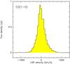 |
Fig. 1 CO(1–0) spectrum of NGC 6240 obtained with IRAM/PdBI in D configuration. Asymmetric broad wings extend from −600 km s-1 to + 800 km s-1 with respect to the systemic velocity. The 3 mm continuum has been subtracted to highlight the high-velocity wings. The spectral channels are 53.3 km s-1 wide. |
2. PdBI observations and data analysis
We observed with the PdBI the CO(1–0) transition, redshifted to 112.516 GHz assuming a systemic velocity of 7339 km s-1 (Iono et al. 2007), corresponding to a redshift of z = 0.02448. The observations were carried out in May 2011 with six antennas using the compact array configuration, and in January 2012 with five antennas in the extended (A) configuration. The on-source time of this dataset is ~4.6 h in the compact configuration and ~5.9 h in the extended configuration.
Data were reduced using GILDAS. The system temperatures during the observations were in the range between 150 and 300 K. The absolute flux calibration relies on the strong quasars 3C273 and 3C279, and its accuracy is expected to be of the order 10% (Castro-Carrizo & Neri 2010). The synthesized beams, obtained by using natural weighting, are 5.6″ × 4.6″ for the D configuration and 1.4″ × 0.7″ for the A configuration maps. The achieved noise levels are 0.9 mJy/beam for the D configuration data, and 1.2 mJy/beam over 20 MHz (i.e. ~50 km s-1) for the configuration A data.
3. X-ray observation and data analysis
NGC 6240 was observed by Chandra on July 2001 for about 35 ks. Reduced and calibrated data are available from the public CXO data archive. Results from these observations have been published by Komossa et al. (2003) and Lira et al. (2004).
4. Results
Figure 1 shows the continuum-subtracted spectrum of the CO(1–0) line, extracted from a polygonal region enclosing the source from the D-array configuration data. The 3 mm continuum was estimated by averaging the visibilities in the spectral channels corresponding to the velocity ranges –3500 to –2000 km s-1, and 2000 to 4000 km s-1 with respect to the systemic velocity. This range of velocities (not shown in Fig. 1 for clarity) is fully covered by the WideX Correlator, and it is free of emission lines. Based on the data taken in the D-array configuration, the continuum emission peaks at −0.16, 0.82 arcsec off the phase tracking center, and it has a flux density of 12.7 mJy. This is consistent with the 1 mm continuum reported by Tacconi et al. (1999), assuming a radio spectral index of 0.7. Two components of the radio and mm continua, centered on the position of each AGN, are found in maps with higher spatial resolution (Tacconi et al. 1999; Colbert et al. 1994). Our data from the D configuration do not allow us to spatially resolve these two components. The continuum map shows one component whose fitted size is 1 ± 0.1 kpc (FWHM), assuming a circular Gaussian model. The 1 mm and radio (8 GHz) continua are consistent with nonthermal synchrotron emission. The CO line peaks close to the assumed systemic velocity (~−50 km s-1). Broad and asymmetric wings extend to at least −600 km s-1 on the blue side and +800 km s-1 an the red side of the line peak. The full width at zero intensity (FWZI ~ 1400 km s-1) is broader than those of CO(2–1) and CO(3–2) reported by Engel et al. (2010) and Iono et al. (2007). In particular, the blue side of the line covers a wider velocity range than the previously reported −450 km s-1 (Bryant & Scoville 1996; Tacconi et al. 1999; Engel et al. 2010; Iono et al. 2007; Nakanishi et al. 2005), probably due to the larger bandwidth and the better sensitivity of the new PdBI receivers.
Figure 2 shows the integrated maps from the D configuration data of the CO core emission (−50 to 50 km s-1) and of the redshifted velocities (from 400 to 800 km s-1 with respect to the systemic velocity). The axes show the coordinate offsets with respect to the phase tracking center, (RA, Dec) = (16:52:58.9, 02:24:02.9). The positions of the two AGN nuclei from VLBI observations (Hagiwara et al. 2011) are also indicated. The CO core emission is elongated in the north-south direction on scales of 10′′, and shows a faint southwestern elongation. The map of the red wing shows a strong compact source of size ~1.7 kpc and cospatial with the narrow core emission, and an elongation in the east-west direction with a position angle of 80 degrees. Fitting an elliptical Gaussian model in the uv-plane gives a flux of 11.4 Jy km s-1 for this high velocity, redshifted component. The uv-fit results are reported in Table 1.
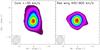 |
Fig. 2 Maps of the CO core emission (left panel, −50, +50 km s-1) and red wing emission (right panel 400 to 800 km s-1 with respect to the systemic velocity), from the compact D array data. Each contour is 5σ (limited to 20σ). The positions of the two AGN nuclei are shown by crosses. The synthesized beam is shown in the bottom-left corners. |
4.1. Blueshifted CO emission
We now examine in detail the blueshifted emission of CO. We find complex morphology extended on scales from a few arcseconds to 15–20′′. Figure 3 shows CO(1–0) maps at different velocities from −400 to −100 km s-1 in channels 20 MHz (=53.3 km s-1) wide for the D and A configuration data. Each contour in Fig. 3 is 5σ (limited to 20σ for clarity). Two structures are particularly prominent: emission extended eastward out to at least 15′′ with velocities from −400 to −200 km s-1, and emission extending southwestward with velocities from −200 to −100 km s-1. The most prominent emission is located eastward from the nuclei, i.e. approximately perpendicular to the line connecting the galactic nuclei, in the velocity range −400 to −150 km s-1. From this, a structure showing velocities of ~−260 km s-1 develops in the southern direction, most likely a tidal tail remnant of the merger. This shows substructure in the form of three main clumps of CO emission, and it coincides with the smooth structure seen by Bush et al. (2008) at 8 μm, and tracing dust through emission by poly-aromatic hydrocarbons (PAHs). Figure 3 (lower panels) shows the maps obtained by merging the data from the D and A configuration. The synthesized beam is intermediate between them both and allows for better spatial resolution of the thin, jet-like structures to better follow their alignment with the emission at other wavelengths. In the merged maps, we estimate, that for the central region (around the nuclei) we are missing ~33% of the flux.
Measured quantities from the uv-plane fit, and derived quantities (line luminosities and gas masses) of the CO-emitting components.
Figure 4 shows two spectra extracted from circular regions of 2′′ radius centered on the eastern and southwestern features. The spectra were extracted from the cleaned data cubes in regions that enclose the extended structures shown in Fig. 3. These spectra are presented for the purpose of showing the emission line peak velocity and linewidth, and should not be used to derive the fluxes. Here we derive the line fluxes from the visibilities of D configuration data. We derive the line intensities of the two blueshifted structures and of the nuclear region by fitting the visibilities of the compact D configuration array data in the uv-plane. The fit in the uv-plane yields the flux at zero spacing. First, we fit the central region around the two nuclei (see Fig. 2, left panel), with the combination of two elliptical Gaussian models, which yield a line intensity of ICO = 213 Jy km s-1 (Table 1). The fit produces a residual table where the visibilities of the central component have been subtracted. To derive the line intensity of the blueshifted, extended structures, we fit the residual visibilities using two elliptical Gaussians. The derived line intensity is 49.3 Jy km s-1 (over 600 km s-1) for the eastern emission region, and 32.5 Jy km s-1 (over 400 km s-1) for the south-western streamer. Summing these three components, we obtain a total integrated CO intensity of 295 ± 29 Jy km s-1, in agreement with both the Solomon et al. (1997) single-dish observations (310 Jy km s-1) and with the interferometric flux (324 Jy km s-1) of Bryant & Scoville (1996).
The emission of each blueshifted region is four to seven times fainter than the central part of the galaxy. As seen in Fig. 3, both these structures are spatially resolved. The eastern component is found to be 7.6″,1.3″ off the phase tracking center. The southwestern one is found at −6.4″, −6.8″ off the phase center. The fit with elliptical Gaussians gives sizes of 14.4″ × 8.2′′ for the eastern blob, and 8.3″ × 4.4′′ for the southwestern blob.
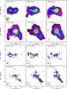 |
Fig. 3 Upper panel: CO(1–0) maps from the compact array data, in velocity bins of 20 MHz each (velocity labels are rounded off), showing the detection of blueshifted CO, including structures extended on scales of 10–15′′. The positions of the two AGN nuclei are shown by crosses. The synthesized beam is shown in only the first panel, for clarity. Each contour is 5σ (limited to 20σ). Lower panel: maps from merged data of the D and A configurations in the same velocity channels. The synthesized beams are shown in the bottom-left corners. |
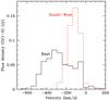 |
Fig. 4 CO(1–0) spectra of NGC 6240 extracted from the D configuration data in circular regions of 2′′ radii encompassing the extended, blueshifted emission eastward (solid black histogram) and southwestward of the nuclei (red dashed histogram). The extraction regions are centered on offsets of (7.6′′, 1.3′′) and (–6.4′′, –6.8′′) from the phase-tracking center. |
Figure 5 (left panel) shows the Wide Field Planetary Camera (WFPC2 F673N) image from the Hubble Space Telescope (HST), which includes the galaxy’s Hα emission (Gerssen et al. 2004), with overlaied contours of the blueshifted CO(1–0) emission at −400 km s-1 and −100 km s-1. The WFPC2 image shows that the Hα nebula comprises five main bright filaments: two southwards of the nuclear region, one located in the western region, and two eastwards from the nuclei. We note that the CO emission with velocity –100 km s-1 is located on the southwestern dust lane, in between two Hα filaments. An elongation of this component toward the northern dust lane is also visible. The CO emission centered at −400 km s-1 first follows the eastern elongation of the Hα emission, and continues further eastward and southward. We also show the X-ray emission at 1.6–2 keV, centered on the highly ionized Si emission. The X-ray data trace the Hα emission remarkably well. In particular, the soft X-ray emission is coincident with the eastern Hα, H2 (see Fig. 9 in Max et al. 2005) and CO elongation. This led us to further investigate the association of the X-ray emission with the Hα, H2, and CO emitting gas.
4.2. X-ray spatially resolved spectroscopy
We extracted a spectrum from the X-ray Chandra data at the position of each of the five Hα filaments described above and combined them. The extraction regions are shown in Fig. 6. A background spectrum was extracted from a source-free region of 25 arcmin2 size at distances of 2 to 5 arcmin from the nuclei of the galaxy, in order to avoid the contamination from the diffuse X-ray emission, which is still seen on scales of 1 arcmin away from the nuclei. The background-subtracted X-ray spectrum is plotted in Fig. 7. Strong emission lines are visible at about 1.3–1.4 keV, 1.7–1.9 keV and 2.3–2.4 keV. At these energies the ionized emission from Mg, Si, and S is expected. We fitted the spectrum using xspec and adopting χ2 statistics. The spectrum was binned to have at least 30 counts per channel. We limited the fit to the 0.5–7 keV band (440 original channels, 67 bins), where the instrument response is best calibrated and where it avoids strong background lines at high energy (see e.g. the Chandra background spectrum in Fiore et al. 2011). We started modeling the spectrum with a thermal equilibrium gas component (mekal in xspec), reduced at low energy by photoelectric absorption by gas along the line of sight. This model is clearly inadequate for reproducing the observed spectrum, giving a χ2 = 179.5 for 63 degrees of freedom (D.O.F.) and large residuals at 0.8–0.9 keV, 1.2 keV, 1.8 keV and above 4 keV. We then added a second thermal equilibrium gas component to the model. Figure 7 shows the best fit model with eight free parameters (two temperatures, two metal abundances, two normalizations, and two absorbing column densities). The best fit χ2 is 93.3 (59 D.O.F.). There are rather strong positive residuals at 1, 1.4, 1.8, 2.2 keV, i.e. the position of the Mg, Si, and S line complexes. Stronger line emission is expected in nonequilibrium models, because of the broader ion distribution with respect to thermal equilibrium models at the same temperature and metal abundances. In particular, shock models, like xspec pshock, are known to produce spectra with prominent line emission. We therefore fitted the spectrum with a model that includes a thermal equilibrium component and a shock component. The best fit χ2 is now 62.1 (58 D.O.F.). The improvement in χ2 with respect to the two component thermal equilibrium model is significant at the 99.9997% confidence level (using the F test). Residuals with respect to the best fit model do not show any systematic deviation. Figure 8 shows the best fit unfolded (i.e. corrected for the response matrix of the instrument) spectrum with the identified contributions of the thermal equilibrium and shock components. We conclude that the X-ray analysis supports the idea that shocked gas is present at the position of strong Hα emission, both in the nuclear starburst and in the elongated filaments.
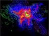 |
Fig. 5 Hα map of NGC 6240 (color image). CO(1–0) emission at different velocities: −350 km s-1 (green contours), −100 km s-1 (magenta contours), with respect to the system velocity. Contours are calculated by merging D and A configuration data. Chandra 1.6–2 keV emission is shown by white contours. |
5. Discussion and conclusions
We have obtained deep 3 mm maps of the archetypical interacting galaxy NGC 6240 with the IRAM PdBI, covering a velocity range of 10 000 km s-1. The CO(1–0) line shows strong blue and red wings extending from −600 km s-1 to +800 km s-1 with respect to the systemic velocity. The line (FWZI = 1400 km s-1) is significantly broader than the one previously reported by Tacconi et al. (1999), Engel et al. (2010), and Iono et al. (2007). The systemic CO emission shows a north-south elongation over at least 10″. Elongation in the same direction is seen in the CO(1–0) maps of Bryant & Scoville (1996) and in the CO(2–1) maps of Tacconi et al. (1999), and Engel et al. (2010) on ten times smaller scales. The CO luminosity of this region is L′(CO) = 5.7 × 10⁹ K km s-1 pc2. We derived an estimate of the molecular gas mass in this region, assuming the standard CO to H2 conversion factor, α = 0.8 M⊙ (K km s-1 pc2)-1 (units omitted hereafter). We found M(H2) = 4.5 109 M⊙, which is consistent with the value derived from CO(2–1) for this region by Tacconi et al. (1999).
We were able to identify new components. We found CO emission extended up to distances of 15–20′′ from the galaxy center (7–10 kpc at the distance of NGC 6240). In particular, we found strong emission blueshifted by ~150 to 400 km s-1 extending eastward by at least 15′′ from the nuclei, and by 100–200 km s-1 extending south-westward on a similar scale. The presence of the latter component was suggested by the interferometric CO maps of Bryant & Scoville (1996), although with low significance.
The CO southwestern emission coincides with the dust lane seen in HST images (Gerssen 2004, also see Fig. 5) and in the IRAC 8 μm image (Bush et al. 2008). This large scale dust distribution has been interpreted as due to a tidal tail curving in front of the system (Gerssen et al. 2004; Yun & Hibbard 2001). Molecular gas is associated with this tidal tail, a situation reminiscent of M 82, where Walter et al. (2002) found molecular gas in the tidal tales correlated with dust absorption features. The integrated CO luminosity of the southwestern emitting region is L′(CO) = 8.7 × 10⁸ K km s-1 pc2. For the conversion from CO luminosity into molecular gas mass M(H2), we conservatively adopted the lowest conversion factor found in the giant outflows and streamers of M 82 (Weiss et al. 2001), α = 0.5. The mass of the molecular gas in this region is thus M(H2) = 4.3 × 10⁸ M⊙, so four to ten times the H2 mass in the streamers of M 82 (Walter et al. 2002, derived for the same conversion factor). This estimate probably represents a lower limit to the molecular gas mass in this streamer. The physical size of the southwestern tidal tail is however at least 15′′, i.e. 7 kpc, four to seven times larger than the streamers in M 82 (Walter et al. 2002). The CO extended emission to the north (see Fig. 2, left panel) coincides with a dust lane seen in HST images (Gerssen et al. 2004) and might be associated with another streamer. The detection of molecular streamer(s) in NGC 6240 confirms that the molecular gas is severely affected by galaxy interaction and that the redistribution of molecular gas is very likely the trigger for the strong starburst activity in the central region of NGC 6240.
The blueshifted eastern CO emitting region is not associated with the dust lanes mentioned above, but follows an Hα filament, and PAH emission observed at 8 μm (Bush et al. 2008). The emission-line nebula seen in Hα images (Gerssen et al. 2004) is interpreted as evidence of a superwind that is shock heating ambient ISM. The Hα emitting filaments are aligned east-westward, perpendicular to the dust lanes and to the line connecting the two nuclei. The X-ray emission is associated with the Hα filaments (Lira et al. 2002). In particular, strong soft X-ray emission is coincident with the northeastern filament (N–E region in Fig. 6). We re-analyzed the Chandra X-ray data and found strong evidence of shocked gas at the position of the Hα filaments. The presence of shocked gas in the NGC 6240 system is confirmed by the detection of strong H2(1–0) S(1) emission at 2.12 μm. NGC 6240 has the strongest H2 line emission found in any galaxy (Goldader et al. 1995). Shocks are usually identified as the excitation mechanism for this line. Ohyama et al. (2000, 2003) suggest that such shocks are produced by a superwind outflowing from the southern nucleus and colliding with the surrounding molecular gas. Intriguingly, Max et al. (2005) find that excited H2 emission closely follows the Hα filament extending eastward. The position of one of the peaks of the eastern blueshifted CO emission coincides with the position where Bland-Hawthorne et al. (1991) and Gerssen et al. (2004) found a large velocity gradient of the ionized gas (the velocity decreasing, roughly, north to south). No significant radio continuum emission is detected in this region in the VLA maps of Colbert et al. (1994). The blueshifted molecular gas in this region might be a tidal tail, left behind during the merger. However, its association with strongly shocked gas suggests that a shock is propagating eastward and is also compressing the molecular gas, while crossing it.
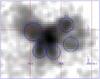 |
Fig. 6 The Chandra X-ray map of NGC 6240 in the energy range 0.3–4 keV. The circles indicate the regions where we extracted the X-ray spectra. The region for the background extraction is outside the limits of this map, at 2–5 arcmin from the nuclei. |
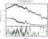 |
Fig. 7 Top panel: the top curve represents the background corrected Chandra spectrum (uncorrected for the response of the instrument; crosses denote spectral widths and amplitude uncertainties) extracted at the position of Hα filaments (see Fig. 6), and fitted with a two-temperature thermal equilibrium model (solid line). The lower curve represents the background spectrum. Data, represented by crosses, have been binned to give a signal-to-noise ratio >5 in each bin (for plotting purposes only). Bottom panel: the data-to-model ratio (the green solid line representing a ratio of unity), showing the residuals at about 1 keV, 1.4 keV, 1.8 keV, 2.2 keV, and 5 keV. |
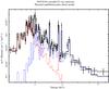 |
Fig. 8 The background-corrected Chandra spectrum (also corrected for the response matrix of the instrument) extracted at the position of the Hα filaments (see Fig. 6). Symbols are as in Fig. 7. Red dotted histogram: thermal equilibrium model component; blue dashed histogram: shock model component. |
The integrated luminosity of CO in this region is L′(CO) = 1.3 × 10⁹ K km s-1 pc2, corresponding to a gas mass M(H2) = 7 × 10⁸ M⊙ (assuming again α = 0.5). Hypothesizing that this outflow originates in the southern, luminous AGN (or from both the AGN), we derive here a mass loss rate. We assume that the molecular outflow is distributed in a spherical volume of radius Rof = 7 kpc (i.e. the distance of the eastern blob from the AGN), centered on the AGN. If the gas is uniformly distributed in this volume, the volume-averaged density of molecular gas is given by  , where Ω is the solid angle subtended by the outflow, and Mof is the mass of gas in the outflow (Feruglio et al. 2010; Maiolino et al. 2012). This assumption is an approximation, and evidently cannot represent the complexity of the system, but can provide a rough estimate of the mass loss rate. Based on this geometry, we can derive a mass loss rate by using the relation:
 where v is the terminal velocity of the outflow (~400 km s-1). This relation yields a mass loss rate of Ṁ ~ 120 M⊙/yr. The Hα, H2, and CO(1–0) maps suggest that the outflow is most likely conical. In this geometry, since the mass loss rate is independent of Ω, the mass outflow rate would be equal to the spherical case if there are no significant losses through the lateral sides of the cone. As it is observed in other local massive outflows (Cicone et al. 2012; Aalto et al. 2012), the outflowing gas is likely characterized by a wide range of densities, ranging from low density gas to dense clumps, which would increase the mass flow rate. In addition, the mass flow rate would obviously be larger than our previous estimates if α is significantly higher than 0.5. To date, this is the lowest conversion factor measured in an extragalactic object. This said, it is unlikely that the mass loss rate is less than several tens M⊙ yr-1, and it is likely as big as a few hundred M⊙ yr-1. The kinetic power of the outflowing gas is given by the relation Pk = 0.5 v2 Ṁ = 6 × 1042 erg s-1. The age of the outflow is >2 × 10⁷ years, since it is observed at about 7 kpc distance from the southern nucleus. The star formation rate at the position of the eastern filament can be evaluated through both the Hα luminosity and the X-ray luminosity (e.g. Kennicut 1998; Ranalli et al. 2003). The 0.5–2 keV X-ray luminosity at the position of the eastern filament is 0.5−1 × 1041 erg s-1, which according to Ranalli et al. (2003) would imply a star formation rate of 10–20 M⊙ yr-1. This estimate is derived by assuming that all the X-ray luminosity is due to star formation. In Sect. 4.2 we showed that at least a fraction of the X-luminosity is due to a shock, therefore the SFR derived from the X-ray is an upper limit. This would suggest that the outflow is not pushed by SN winds. Indeed, the power transferred to the ISM by a star formation-driven wind is given by PSF = η × 7 × 1041 × SFR = 1042 erg s-1, where η ~ 0.1 is the standard mass-energy conversion (see e.g. Lapi et al. 2005). We conclude that it is unlikely that the molecular flow is powered by star formation. Instead, star formation in this region is likely to be in the process of being quenched by the outflow. However, we cannot exclude that star formation in this area is induced by the compression caused by the propagating shock.
We detected a redshifted component with velocity 400 to 800 km s-1 with respect to the systemic velocity (Fig. 2), centered on the two AGN nuclei. Interestingly this emitting region is elongated in the same east-west direction as the blueshifted emission discussed above, although on smaller scales (~1.7 kpc in diameter). We derive a CO luminosity for this component of L′(CO) = 3.0 × 10⁸ K km s-1 pc2, which converts into a gas mass of M(H2) = 1.5 × 10⁸ M⊙, under the same assumptions as given above for the CO-to-H2 conversion factor. The high velocity of this component suggests that the AGN might contribute to the dynamics of this gas (Sturm et al. 2011).
Given the complex dynamics and morphology of this system, it is not trivial to disentangle and quantify the relative role of each mechanism. Probably several mechanisms are acting contiguously, but mainly the radiation pressure of the AGN together with dynamic shocks induced by the merger event. High-resolution, X-ray observations will help clarify the interaction between the star-forming regions and the CO extended structures (Wang et al. in prep., conf. comm.). The high spatial resolution data taken in the A-array configuration indeed provide new insights into the nuclear region, which will be addressed in a separate publication (Feruglio et al., in prep.).
Acknowledgments
We thank D. Downes and R. Neri for useful inputs and careful reading of the paper. F.F. acknowledges support from PRIN-INAF 2011. We acknowledge the referee for her/his very careful review, that allowed us to significantly improve the quality of this work.
References
- Aalto, S., Garcia-Burillo, S., Muller, S., et al. 2012, A&A, 537, 44 [Google Scholar]
- Alatalo, K. A., Davis, T. A., Young, L. M., et al. 2011, ApJ, 735, 88 [NASA ADS] [CrossRef] [Google Scholar]
- Barnes, J. E., & Hernquist, L. 1996, ApJ, 471, 115 [NASA ADS] [CrossRef] [Google Scholar]
- Bland-Hawthorn, J., Wilson, A. S., & Cecil, G. 1991, ApJ, 371, 19 [NASA ADS] [CrossRef] [Google Scholar]
- Boroson, T., & Meyers, K. 1992, ApJ, 397, 442 [NASA ADS] [CrossRef] [Google Scholar]
- Bryant, P. M., & Scoville, N. Z. 1996, ApJ, 457, 678 [NASA ADS] [CrossRef] [Google Scholar]
- Bush, S. J., Wang, Z., Karovska, M., & Fazio, G. 2008, ApJ, 688, 875 [NASA ADS] [CrossRef] [Google Scholar]
- Carilli, C. L., Wrobel, J. M., & Ulvestad, J. S. 1998, AJ, 115, 928 [NASA ADS] [CrossRef] [Google Scholar]
- Castro-Carrizo, A., & Neri, R. 2010, IRAM Plateau de Bure Interferometer Data Reduction Cookbook [Google Scholar]
- Cavaliere, A., & Vittorini, V. 2000, ApJ, 543, 599 [NASA ADS] [CrossRef] [Google Scholar]
- Cicone, C., Feruglio, C., Maiolino, R., et al. 2012, A&A, 543, A99 [NASA ADS] [CrossRef] [EDP Sciences] [Google Scholar]
- Colbert, E. J. M., Wilson, A. S., & Bland-Hawthorn, J. 1994, ApJ, 436, 89 [NASA ADS] [CrossRef] [Google Scholar]
- Croton, D. J., Springel, V., White, S. D. M., et al. 2006, MNRAS, 367, 864 [NASA ADS] [CrossRef] [Google Scholar]
- Daddi, E., Alexander, D. M., Dickinson, M., et al. 2007, ApJ, 670, 173 [NASA ADS] [CrossRef] [Google Scholar]
- Davies, R. I., Tacconi, L. J., & Genzel, R. 2004, ApJ, 613, 781 [NASA ADS] [CrossRef] [Google Scholar]
- Davies, R. I., Sternberg, A., Lehnert, M. D., & Tacconi-Garman, L. E. 2005, ApJ, 633, 105 [NASA ADS] [CrossRef] [Google Scholar]
- Dekel, A., Birnboim, Y., Engel, G., et al. 2009, Nature, 457, 451 [NASA ADS] [CrossRef] [PubMed] [Google Scholar]
- Di Matteo, T., Springel, V., & Hernquist, L. 2005, Nature, 433, 604 [NASA ADS] [CrossRef] [PubMed] [Google Scholar]
- Downes, D., & Solomon, P. M. 1998, ApJ, 507, 615 [NASA ADS] [CrossRef] [Google Scholar]
- Elbaz, D., Dickinson, M., Hwang, H. S., et al. 2011, A&A, 533, A119 [NASA ADS] [CrossRef] [EDP Sciences] [Google Scholar]
- Engel, H., Davies, R. I., Genzel, R., et al. 2010, A&A, 524, A56 [NASA ADS] [CrossRef] [EDP Sciences] [Google Scholar]
- Fabian, A. C. 1999, MNRAS, 308, 39 [Google Scholar]
- Feruglio, C., Maiolino, R., Piconcelli, E., et al. 2010, A&A, 518, A155 [Google Scholar]
- Fiore, F., Puccetti, S., Grazian, A., et al. 2012, A&A, 537, A16 [NASA ADS] [CrossRef] [EDP Sciences] [Google Scholar]
- Fischer, J., Sturm, E., Gonzales-Alfonso, E., et al. 2010, A&A, 518, A41 [Google Scholar]
- Gerssen, J., van der Marel, R. P., Axon, D., et al. 2004, AJ, 127, 75 [NASA ADS] [CrossRef] [Google Scholar]
- Granato, G. L., De Zotti, G., Silva, L., et al. 2004, ApJ, 600, 580 [Google Scholar]
- Goldader, J. D., Joseph, R. D., Doyon, R., & Sanders, D. B. 1995, ApJ, 444, 97 [NASA ADS] [CrossRef] [Google Scholar]
- Hagiwara, Y., Baan, W. A., & Klockner, H. 2011, AJ, 142, 17 [NASA ADS] [CrossRef] [Google Scholar]
- Iono, D., Wilson, C. D., Takakuwa, S., et al. 2007, ApJ, 659, 283 [NASA ADS] [CrossRef] [Google Scholar]
- Kauffmann, G., Heckman, T. M., Tremonti, C., et al. 2003, MNRAS, 346, 1055 [Google Scholar]
- Kennicut, R. C. 1998, ApJ, 498, 541 [NASA ADS] [CrossRef] [Google Scholar]
- King, A. R. 2005, ApJ, 635, 121 [Google Scholar]
- King, A. R. 2010, MNRAS, 402, 1516 [NASA ADS] [CrossRef] [Google Scholar]
- Komossa, S., Burwitz, V., Hasinger, G., et al. 2003, ApJ, 582, 15 [Google Scholar]
- Lapi, A., Cavaliere, A., & Menci, N. 2005, ApJ, 619, 60 [NASA ADS] [CrossRef] [Google Scholar]
- Lira, P., Ward, M. J., Zezas, A., & Murray, S. S. 2002, MNRAS, 330, 259 [NASA ADS] [CrossRef] [Google Scholar]
- Maiolino, R., Gallerani, S., Neri, R., et al. 2012, MNRAS, 425, L66 [NASA ADS] [CrossRef] [Google Scholar]
- Max, C. E., Canalizo, G., Macintosh, B. A., et al. 2005, ApJ, 621, 738 [NASA ADS] [CrossRef] [Google Scholar]
- Menci, N., Fontana, A., Giallongo, E., et al. 2006, ApJ, 647, 753 [NASA ADS] [CrossRef] [Google Scholar]
- Menci, N., Fiore, F., Puccetti, S., & Cavaliere, A. 2008, ApJ, 686, 219 [NASA ADS] [CrossRef] [Google Scholar]
- Mihos, J. C., & Hernquist, L. 1996, ApJ, 464, 641 [NASA ADS] [CrossRef] [Google Scholar]
- Nakanishi, K., Okomura, S. K., Kohno, K., Kawabe, R., & Nakagawa, T. 2005, PASJ, 57, 575 [NASA ADS] [CrossRef] [Google Scholar]
- Ohyama, Y., Yoshida, M., Takata, T., et al. 2000, PASJ, 52, 563 [NASA ADS] [Google Scholar]
- Ohyama, Y., Yoshida, M., & Takata, T. 2003, AJ, 126, 229 [Google Scholar]
- Peng, Y., Lilly, S., Kovac, K., et al. 2010, ApJ, 721, 193 [NASA ADS] [CrossRef] [Google Scholar]
- Ranalli, P., Comastri, A., & Setti, G. 2003, A&A, 399, 39 [NASA ADS] [CrossRef] [EDP Sciences] [Google Scholar]
- Rodighiero, G., Daddi, E., Baronchelli, I., et al. 2011, ApJ, 739, 40 [NASA ADS] [CrossRef] [Google Scholar]
- Sakamoto, K., Aalto, S., Wilner, D. J., et al. 2009, ApJ, 700, 104 [Google Scholar]
- Sanders, D. B., & Mirabel, I. F. 1996, ARA&A, 34, 749 [NASA ADS] [CrossRef] [Google Scholar]
- Sanders, D. B., Soifer, B. T., Elias, J. H., et al. 1988, ApJ, 325, 74 [NASA ADS] [CrossRef] [Google Scholar]
- Scoville, N. Z., Frayer, D. T., Schinnerer, E., & Christopher, M. 2003, ApJ, 585, L105 [NASA ADS] [CrossRef] [Google Scholar]
- Silk, J., & Rees, M. J. 1998, A&A, 331, L1 [NASA ADS] [Google Scholar]
- Sturm, E., Gonzalez-Alfonso, E., Veilleux, S., et al. 2011, A&A, 518, A36 [Google Scholar]
- Solomon, P. M., & Van den Bout, P. A. 2005, ARA&A, 43, 677 [NASA ADS] [CrossRef] [Google Scholar]
- Solomon, P. M., Downes, D., Radford, S. J. E., et al. 1997, ApJ, 478, 144 [NASA ADS] [CrossRef] [Google Scholar]
- Solomon, P. M., Downes, D., Radford, S. J. E., & Barret, J. W. 2007, ApJ, 478, 144 [Google Scholar]
- Tacconi, L., Genzel, R., Tezca, M., & Gallimore, J. F. 1999, ApJ, 524, 732 [NASA ADS] [CrossRef] [Google Scholar]
- Veilleux, S., Cecil, G., & Bland-Hawthorn, J. 2005, ARA&A, 43, 769 [Google Scholar]
- Vignati, P., Molendi, S., Matt, G., et al. 1999, A&A, 349, 57 [Google Scholar]
- Walter, F., Weiss, A., & Scoville, N. 2002, ApJ, 580, 21 [Google Scholar]
- Weiss, A., Neininger, N., Húttemeister, S., & Klein, U. 2001, A&A, 365, 571 [NASA ADS] [CrossRef] [EDP Sciences] [Google Scholar]
- Yun, M. S., & Hibbard, J. E. 2001, in Gas and Galaxy Evolution, eds. J. E. Hibbard, M. Rupen, & J. H. van Gorkom, ASP Conf. Proc., 240, 866 [Google Scholar]
- Zubovas, K., & King, A 2012, ApJ, 745, 34 [Google Scholar]
All Tables
Measured quantities from the uv-plane fit, and derived quantities (line luminosities and gas masses) of the CO-emitting components.
All Figures
|
Fig. 1 CO(1–0) spectrum of NGC 6240 obtained with IRAM/PdBI in D configuration. Asymmetric broad wings extend from −600 km s-1 to + 800 km s-1 with respect to the systemic velocity. The 3 mm continuum has been subtracted to highlight the high-velocity wings. The spectral channels are 53.3 km s-1 wide. |
| In the text | |
|
Fig. 2 Maps of the CO core emission (left panel, −50, +50 km s-1) and red wing emission (right panel 400 to 800 km s-1 with respect to the systemic velocity), from the compact D array data. Each contour is 5σ (limited to 20σ). The positions of the two AGN nuclei are shown by crosses. The synthesized beam is shown in the bottom-left corners. |
| In the text | |
|
Fig. 3 Upper panel: CO(1–0) maps from the compact array data, in velocity bins of 20 MHz each (velocity labels are rounded off), showing the detection of blueshifted CO, including structures extended on scales of 10–15′′. The positions of the two AGN nuclei are shown by crosses. The synthesized beam is shown in only the first panel, for clarity. Each contour is 5σ (limited to 20σ). Lower panel: maps from merged data of the D and A configurations in the same velocity channels. The synthesized beams are shown in the bottom-left corners. |
| In the text | |
|
Fig. 4 CO(1–0) spectra of NGC 6240 extracted from the D configuration data in circular regions of 2′′ radii encompassing the extended, blueshifted emission eastward (solid black histogram) and southwestward of the nuclei (red dashed histogram). The extraction regions are centered on offsets of (7.6′′, 1.3′′) and (–6.4′′, –6.8′′) from the phase-tracking center. |
| In the text | |
|
Fig. 5 Hα map of NGC 6240 (color image). CO(1–0) emission at different velocities: −350 km s-1 (green contours), −100 km s-1 (magenta contours), with respect to the system velocity. Contours are calculated by merging D and A configuration data. Chandra 1.6–2 keV emission is shown by white contours. |
| In the text | |
|
Fig. 6 The Chandra X-ray map of NGC 6240 in the energy range 0.3–4 keV. The circles indicate the regions where we extracted the X-ray spectra. The region for the background extraction is outside the limits of this map, at 2–5 arcmin from the nuclei. |
| In the text | |
|
Fig. 7 Top panel: the top curve represents the background corrected Chandra spectrum (uncorrected for the response of the instrument; crosses denote spectral widths and amplitude uncertainties) extracted at the position of Hα filaments (see Fig. 6), and fitted with a two-temperature thermal equilibrium model (solid line). The lower curve represents the background spectrum. Data, represented by crosses, have been binned to give a signal-to-noise ratio >5 in each bin (for plotting purposes only). Bottom panel: the data-to-model ratio (the green solid line representing a ratio of unity), showing the residuals at about 1 keV, 1.4 keV, 1.8 keV, 2.2 keV, and 5 keV. |
| In the text | |
|
Fig. 8 The background-corrected Chandra spectrum (also corrected for the response matrix of the instrument) extracted at the position of the Hα filaments (see Fig. 6). Symbols are as in Fig. 7. Red dotted histogram: thermal equilibrium model component; blue dashed histogram: shock model component. |
| In the text | |
Current usage metrics show cumulative count of Article Views (full-text article views including HTML views, PDF and ePub downloads, according to the available data) and Abstracts Views on Vision4Press platform.
Data correspond to usage on the plateform after 2015. The current usage metrics is available 48-96 hours after online publication and is updated daily on week days.
Initial download of the metrics may take a while.