| Issue |
A&A
Volume 548, December 2012
|
|
|---|---|---|
| Article Number | A95 | |
| Number of page(s) | 18 | |
| Section | Stellar atmospheres | |
| DOI | https://doi.org/10.1051/0004-6361/201220215 | |
| Published online | 29 November 2012 | |
The magnetic field topology of the weak-lined T Tauri star V410 Tauri
New strategies for Zeeman-Doppler imaging⋆
1
Leibniz-Institute for Astrophysics Potsdam,
An der Sternwarte 16,
14482
Potsdam,
Germany
e-mail: This email address is being protected from spambots. You need JavaScript enabled to view it.
; This email address is being protected from spambots. You need JavaScript enabled to view it.
; This email address is being protected from spambots. You need JavaScript enabled to view it.
2
Department of Physics, Brandon University,
Brandon, Manitoba
R7A 6A9,
Canada
e-mail: This email address is being protected from spambots. You need JavaScript enabled to view it.
Received:
13
August
2012
Accepted:
25
October
2012
Abstract
Aims. In a follow-up investigation we present Zeeman-Doppler maps of the weak-lined T Tauri star (WTTS) V410 Tau. As a rapid rotating star and a typical WTTS the stellar surface of V410 Tau is accessible to surface imaging techniques and allows us to detect and reconstruct the major magnetic surface features on this pre-main sequence star.
Methods. The polarized signals we are measuring are on the order of 10-4 to 10-3 and are hidden well below the noise level of a single observation. A new line profile reconstruction technique based on a singular value decomposition (SVD) allows us to extract the weak polarized line profiles (Stokes V) as well as the intensity profiles (Stokes I). One of the key features of the line profile reconstruction is that the SVD line profiles are amenable to radiative transfer modeling within our Zeeman-Doppler Imaging code iMap. The code also utilizes a new iterative regularization scheme which is independent of any additional surface constraints. To provide more stability a vital part of our inversion strategy is to invert both Stokes I and Stokes V profiles to simultaneously reconstruct the temperature and magnetic field surface distribution of V410 Tau. A new image-shear analysis is also implemented to allow the search for image and line profile distortions induced by a differential rotation of the star.
Results. The magnetic field structure we obtain for V410 Tau shows a good spatial correlation with the surface temperature and is dominated by a strong field within the cool polar spot. The Zeeman-Doppler maps exhibit a large-scale organization of both polarities around the polar cap in the form of a twisted bipolar structure. The magnetic field reaches a value of almost 2 kG within the polar region but smaller fields are also present down to lower latitudes. The pronounced non-axisymmetric field structure and the non-detection of a differential rotation for V410 Tau supports the idea of an underlying α2-type dynamo, which is predicted for WTTS.
Key words: stars: magnetic field / stars: activity / methods: data analysis / line: profiles / techniques: spectroscopic / stars: pre-main sequence
Appendices are available in electronic form at http://www.aanda.org
© ESO, 2012
1. Introduction
T Tauri stars are very young stars on their way toward the zero-age main sequence (ZAMS). With the ongoing contraction they prepare the conditions in their interiors to start the first nuclear process. In classical T Tauri stars, the outside is still dominated by the accretion of matter from the disk while in the weak-lined T Tauri stars (WTTS), or “naked” T Tauri stars, the accretion disk is basically gone and the star is soon to arrive on the ZAMS. Little is known about the magnetic field generating processes during both of these evolutionary phases (see, e.g. the review by Gregory & Donati 2011). How do WTTS stars produce, maintain, and reorganize their internal fields at this rapidly changing evolutionary stage? An even more relevant question from a general point of view is how do these fields manifest themselves on the surface of the star and whether their appearance, i.e. the topology, is directly linked to the generating process in the interior? Or do convection and other surface flows alter the surface appearance in such a way that they will prevent us from making any direct conclusions about the internal dynamo processes? We are still far from answering all these questions which is, unfortunately, not only true for WTTS stars but also for any other type of star (Schrijver & Zwaan 2000). Even for the Sun there is no clear answer yet of how strong sunspots and active regions are still connected deep down into the tachocline region (Rempel & Schüssler 2009; Rempel 2011) where the internal dynamo is believed to operate (Schrijver & Title 1999; Schüssler 2005). We are still in the phase of characterization and it may still take some time before we can connect observations with theory (and vice versa) in a conclusive way.
However, the characterization of surface magnetic fields with techniques like Doppler imaging (DI; e.g. Rice 2002), which tracks the magnetically induced cool spots on the surface of stars, or more directly with Zeeman-Doppler imaging (ZDI; see, e.g. Donati 2001, has provided us in the last two decades with a wealth of new information about the surface spots and magnetic fields on many different types of stars, see Strassmeier (2009) and Donati & Landstreet (2009) for comprehensive overviews.
In this work, we concentrate on DI and ZDI of V410 Tau, a rapidly rotating WTTS that has fully stripped away its surrounding disk. Many WTTS like V410 Tau show strong signatures of photospheric variability attributed to atmospheric magnetic activity rather than to a left-over from external accretion processes. Indirect signs of magnetic activity are known for a long time from photometric light curve variations (see, e.g. Rydgren & Vrba 1983; Bouvier & Bertout 1989). More direct evidence of photospheric magnetic activity could be obtained by Doppler images, in particular for V410 Tau (Joncour et al. 1994; Strassmeier et al. 1994; Hatzes 1995; Rice & Strassmeier 1996; Rice et al. 2011). Skelly et al. (2010) presented the first Zeeman-Doppler map of V410 Tau. Surprisingly, the reconstructed large-scale field exhibit a rather complex structure dispersed over different latitudes with strongly inclined fields that are only weakly correlated with the spots shown in their brightness maps.
Signs of chromospheric and coronal activity on V410 Tau are also known for many years and strong ultraviolet and optical emission lines and X-rays emission were observed (Hatzes 1995; Stelzer & Neuhäuser 2001; Stelzer et al. 2003). An intriguing fact here is that the modulation of the chromospheric and coronal activity tracers seem not to be strongly correlated with the photospheric spot locations (Stelzer et al. 2003).
To shed more light on the magnetic field distribution on stellar surfaces, in particular for V410 Tau, we conducted a simultaneous investigation of rotationally modulated spectral line profiles (Stokes I) and spectropolarimetric line profiles (Stokes V) in terms of a rigorous Doppler imaging and Zeeman-Doppler imaging analysis. In this respect, the present paper is a continuation of the work by Rice et al. (2011), which we hereby call Paper I. The present paper is organized as follows. In Sect. 2, we briefly describe the acquisition of the data. In Sect. 3, we introduce our improved polarized-line profile extraction and reconstruction technique based on a singular-value decomposition (SVD). Section 4 is devoted to a recap of the basic outline and assumptions in our ZDI code iMap and its recent improvements. In Sect. 5, we present the results of our simultaneous DI and ZDI approach as well as the results of our search for a differential rotation on V410 Tau. Section 6 summarizes our findings and conclusions.
2. Observations
High-resolution spectropolarimetric observations were obtained with the ESPADONS echelle
spectrograph and polarimeter (Donati 2003) in
Stokes I and Stokes V at the 3.6 m Canada-France-Hawaii
telescope (CFHT) on Mauna Kea, Hawaii. Data were obtained in queue mode during one observing
block over four nights from 2008 October 15 to 19, and one over 13 nights distributed
between the dates of 2008, December 5th to 2009, January 14th. A spectral resolution of
60 000 with a wavelength coverage of 390–900 nm was obtained. All integrations on V410 Tau
( ) were set to an exposure time of
4 × 600 s. This allowed for a total of 17 spectra with an average signal-to-noise ratio
(S/N) of around 160:1 per single exposure per pixel. All spectra were reduced and extracted
using the Libre-ESPRIT package provided by CFHT and executed automatically. Details of this
reduction procedure are given in Donati et al.
(1997).
) were set to an exposure time of
4 × 600 s. This allowed for a total of 17 spectra with an average signal-to-noise ratio
(S/N) of around 160:1 per single exposure per pixel. All spectra were reduced and extracted
using the Libre-ESPRIT package provided by CFHT and executed automatically. Details of this
reduction procedure are given in Donati et al.
(1997).
3. SVD based signal extraction and reconstruction
3.1. Method
For most active cool late-type stars the typical signal amplitude of a single polarized line profile is on the order of a few times 10-4 relative to the normalized continuum. These values are far below the S/N of a typical spectropolarimetric observation, which hardly exceeds a few times 103. So the individual polarimetric line profiles are buried well below the noise level by typically one order of magnitude. This requires techniques that are able to recover and extract the line profile signals from the measurement noise prior to the actual ZDI analysis. Most of the techniques for circularized, i.e. Stokes V, line profiles take advantage of the fact that the polarized Stokes V patterns for almost all Zeeman sensitive atomic spectral lines are similar except for a non-linear scaling (in wavelength and amplitude) caused by different atomic line parameters, broadening mechanisms, and magnetic sensitivities. For rapidly rotating stars, when the rotational broadening dominates as well as under the weak magnetic field approximation (Stenflo 1994), line-profile shapes can be considered as equal and amplitudes are only linearly dependent upon their individual Landé factors and line strengths. One popular and very successful extraction technique which follows this line of arguments is the so called least-squares deconvolution (LSD, Donati et al. 1997; Kochukhov et al. 2010). Another method is the principal component analysis (PCA, Carroll et al. 2007; Martínez González et al. 2008; Carroll et al. 2009; Paletou 2012) or the simple but very effective coherent addition of line profiles in the velocity or logarithmic wavelength domain (Semel et al. 2009; Ramírez et al. 2010).
For our application to V410 Tau, we present here an improved version of the PCA technique that is more robust in the case of weak polarimetric signals and which can be described in terms of an eigenvalue decomposition (EVD) of the observation covariance matrix. An EVD of the signal covariance matrix (or a SVD of the observation matrix) allows us to obtain an orthogonal decomposition of the signal or line profiles in terms of the covariance eigenprofiles. The basic idea is similar as in the previous PCA-based approach where the similarity of the individual Stokes V profiles allows one to describe the most coherent and systematic features present in all spectral line profiles as a projection onto a small number of eigenprofiles. In parallel, incoherent features like noise, and line blends etc. will be dispersed along many dimensions in the transformed eigenspace. In other words the similarity and coherence of all individual Stokes V patterns allows one to capture the signal pattern by a low-rank representation of the observation covariance matrix. The respective eigenvalues of the observation covariance matrix, together with an estimate of the noise level in the data, then provide a means of separating the low-dimensional signal subspace from the noise subspace. Once the reduced rank of the signal subspace is determined a projection of the observed line profiles onto the signal subspace and a subsequent subspace-averaging is performed to eventually provide the signal boosting effect for the polarimetric line profile. What is described in the following for Stokes V profiles also holds for Stokes I but for the sake of brevity we will use a notation that makes use of Stokes V only.
The problem setup is as follows: an individual, observed, line profile
 is the
result of the true signal vector V(λ) and a
noise vector N, which we consider as additive and
independent of wavelength and time and of zero mean. Although our idealize assumption are
not met (and we will discuss the consequence later in this section), let us proceed with
this assumption to describe the basic mechanism of the subspace method.
is the
result of the true signal vector V(λ) and a
noise vector N, which we consider as additive and
independent of wavelength and time and of zero mean. Although our idealize assumption are
not met (and we will discuss the consequence later in this section), let us proceed with
this assumption to describe the basic mechanism of the subspace method.
The observed line profile can be written in a discrete form as,  (1)where
i and j denote the wavelength and the spectral line
index, respectively. In vector form, we may write Eq. (1) as
(1)where
i and j denote the wavelength and the spectral line
index, respectively. In vector form, we may write Eq. (1) as  (2)We further assume
that the net circular polarization of each individual Stokes V line
profile is zero such that their integral over the wavelength range is also zero. This
implies that there are no gradients in magnetic field and velocity present in the
atmosphere (Carroll & Kopf 2007) which is
also the usual starting point for ZDI to keep the problem tractable.
(2)We further assume
that the net circular polarization of each individual Stokes V line
profile is zero such that their integral over the wavelength range is also zero. This
implies that there are no gradients in magnetic field and velocity present in the
atmosphere (Carroll & Kopf 2007) which is
also the usual starting point for ZDI to keep the problem tractable.
Arranging now the individual, observed, Stokes profiles in a
m × n observation matrix
 ,
where m denotes the number of wavelength pixels and n
the number of observed individual spectral lines, we can calculate the non-normalized
covariance matrix of the observations as
,
where m denotes the number of wavelength pixels and n
the number of observed individual spectral lines, we can calculate the non-normalized
covariance matrix of the observations as  (3)where the
superscript T denotes the transpose. The covariance matrix
(3)where the
superscript T denotes the transpose. The covariance matrix
 is a m × m real symmetric matrix and has
m linear independent eigenvectors, which can be used to decompose
by a spectral decomposition, i.e. an EVD, such as
is a m × m real symmetric matrix and has
m linear independent eigenvectors, which can be used to decompose
by a spectral decomposition, i.e. an EVD, such as  (4)with
 being a diagonal matrix containing the eigenvalues
  ,
and Q an m × m orthogonal
matrix containing in each column the eigenvectors
,
and Q an m × m orthogonal
matrix containing in each column the eigenvectors  . By assumption, signal
and noise are uncorrelated and we may therefore write the covariance matrix
as the sum of the two matrices CS and
CN, i.e. the clean signal and the noise covariance
matrix:
. By assumption, signal
and noise are uncorrelated and we may therefore write the covariance matrix
as the sum of the two matrices CS and
CN, i.e. the clean signal and the noise covariance
matrix:  (5)Based on our assumption
that the clean signals span only a lower dimensional subspace of the observed space (i.e.
signals plus noise), which is equivalent of assuming that the signal matrix is rank
deficient, we can use the orthogonal matrix Q of the observed
signal space for the EVD of the clean signal covariance matrix
CS and the noise covariance matrix
CN, to write
(5)Based on our assumption
that the clean signals span only a lower dimensional subspace of the observed space (i.e.
signals plus noise), which is equivalent of assuming that the signal matrix is rank
deficient, we can use the orthogonal matrix Q of the observed
signal space for the EVD of the clean signal covariance matrix
CS and the noise covariance matrix
CN, to write  (6)and
  (7)which directly
follows from Eq. (5). Here,
σ2 is the eigenvalue of the noise and corresponds to the
noise variance along a direction in subspace, the matrix I is the
identity matrix and ΛS is the diagonal matrix of the
eigenvalues λ of the clean signal matrix. Note, because the noise is
assumed to be isotropic and featureless it will be homogeneously distributed across the
eigenspace with all eigenvalues of similar magnitude. Note also that by definition of the
covariance matrix each eigenvalue provide the total energy (variance) of the observation
along its corresponding dimension (eigenprofile). The noise eigenvalue is related to the
estimated observation error σobs by
(7)which directly
follows from Eq. (5). Here,
σ2 is the eigenvalue of the noise and corresponds to the
noise variance along a direction in subspace, the matrix I is the
identity matrix and ΛS is the diagonal matrix of the
eigenvalues λ of the clean signal matrix. Note, because the noise is
assumed to be isotropic and featureless it will be homogeneously distributed across the
eigenspace with all eigenvalues of similar magnitude. Note also that by definition of the
covariance matrix each eigenvalue provide the total energy (variance) of the observation
along its corresponding dimension (eigenprofile). The noise eigenvalue is related to the
estimated observation error σobs by  (8)Using the definition of
Eqs. (6) and (7) the EVD of the covariance matrix
can now be written as
(8)Using the definition of
Eqs. (6) and (7) the EVD of the covariance matrix
can now be written as 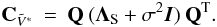 (9)If the clean signals
are confined to an s-dimensional subspace with
s < m, then the eigenvalues of
(9)If the clean signals
are confined to an s-dimensional subspace with
s < m, then the eigenvalues of
 can be expressed as
 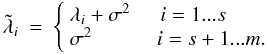 (10)Partitioning
Q in an orthogonal m × s
matrix QS for the signal subspace and a
m × (m − s) matrix
QN for the noise subspace allows us to write for the
observational covariance matrix
(10)Partitioning
Q in an orthogonal m × s
matrix QS for the signal subspace and a
m × (m − s) matrix
QN for the noise subspace allows us to write for the
observational covariance matrix ![Mathematical equation: \begin{equation} {\bf C}_{\tilde{V}^*} \: = \: \left [ {\bf Q}_{\rm S} {\bf Q}_{\rm N} \right ] \: \left ( \: \left [ \begin{array}{cc} \vec{\Lambda}_s & 0 \\ 0 & 0 \end{array} \right ] + \sigma^2 \left [ \begin{array}{cc} \vec{I}_s & 0 \\ 0 & \vec{I}_{m-s} \end{array} \right ] \: \right ) \: \left [ \vec{Q}_{\rm S} \vec{Q}_{\rm N} \right ]^{\rm T}. \label{Eq:3_11} \end{equation}](/articles/aa/full_html/2012/12/aa20215-12/aa20215-12-eq48.png) (11)From this we can
define a simple but effective criterion for the separation of the signal subspace. All
those eigenvalues λi, i.e. the combination of
clean signal and noise eigenvalues, which are larger than the noise eigenvalues alone
carry more energy than a pure noise component and may therefore exhibit significant
structural information. The condition for the separation of the signal space then reads
(11)From this we can
define a simple but effective criterion for the separation of the signal subspace. All
those eigenvalues λi, i.e. the combination of
clean signal and noise eigenvalues, which are larger than the noise eigenvalues alone
carry more energy than a pure noise component and may therefore exhibit significant
structural information. The condition for the separation of the signal space then reads
 (12)It provides an
estimate of the number s of the signal space, i.e. the reduced rank. The
above described EVD can efficiently calculated by utilizing a SVD of the original
observation matrix
(12)It provides an
estimate of the number s of the signal space, i.e. the reduced rank. The
above described EVD can efficiently calculated by utilizing a SVD of the original
observation matrix  .
.
Let us now briefly discuss the restriction and consequences of our idealized assumption, i.e. that we deal with homogeneous and stationary noise. The real noise that we are dealing with in our spectral data is certainly not stationary and may have a dependence on wavelength. The noise can therefore introduce a systematic feature and the noise matrix will have off-diagonal elements. If the correlation of this feature is strong enough among the contributing lines it would give rise to a structure in signal space that is different from pure random noise. In that case this systematic will therefore be detected as a significant signal feature in our framework as it follows our basic notion of being systematic and correlated among all contributing lines. So without giving up the derivation of the rank estimation we need to change the meaning of the signal space. The signal space is not exclusively given by the true underlying Stokes signal but rather includes all systematic effects that possess a certain correlation within the observation matrix.
In principle, we could now retrieve each individual Stokes V profile by
projecting the observed line profiles
Vj onto the restricted set of
s signal eigenprofiles from QS.
This could be done for any line profile of interest. Unfortunately, this approach alone is
limited to relative noise levels above unity. The situation changes when the original
profiles are noise dominated such that the true signal patterns are completely hidden by
noise and any projection operations is increasingly affected by the noise contamination of
the original signal. For this case we use a two-stage strategy where the reduced rank
estimation of the covariance matrix is used to perform a coherent addition of the
projection coefficients in signal subspace. Consequently our second stage of the signal
extraction consists of a projection of each individual line profile onto the eigenprofiles
QS in order to obtain a low-dimensional
representation of each observation vector. This projection and the respective matrix of
projection coefficients VP can be written as
 (13)We can use the
projection matrix to obtain the subspace averaged projection vector
(13)We can use the
projection matrix to obtain the subspace averaged projection vector
 by multiplying an
n × 1 sum vector Z to the projection
matrix VP. Each entry of the vector
Z may hold a specific weighting for each individual
spectral line or may be given by a simple equal weighting scheme (e.g.
1/n for the sample mean).
by multiplying an
n × 1 sum vector Z to the projection
matrix VP. Each entry of the vector
Z may hold a specific weighting for each individual
spectral line or may be given by a simple equal weighting scheme (e.g.
1/n for the sample mean).  (14)We can then use the
averaged projection vector together with the
signal space eigenprofiles to finally obtain the signal
reconstruction VR,
(14)We can then use the
averaged projection vector together with the
signal space eigenprofiles to finally obtain the signal
reconstruction VR,  (15)Now we have a
reconstructed (weighted) mean line profile that is comparable to the mean Zeeman feature
obtained by a conventional LSD approach. However, the reconstruction here is performed
over the estimated signal subspace, which carries the majority of the significant
information of the profile pattern. This is in contrast to the LSD method which operates
in the original data domain where the observed signals are still a mixture of coherent and
non-coherent features. Much of the noise and incoherent structures are already reduced in
the first processing step while the main signal-boosting is provided by Eq. (14). The second crucial difference lies in the
fact that we use this subspace-averaged line profile not as a proxy for the general line
shape in the ZDI inversion but rather as the real approximate mean line
profile that can be synthetically calculated by using the same lines that have been used
for the observation matrix .
Even though it is a formidable computational task to calculate the mean line profile from
several hundreds or even thousands of individual spectral lines in each iteration cycle of
the inversion process it has been shown that artificial neural networks (Bishop 1995) provide a fast and accurate approximation
of the polarized radiative transfer equation to calculate thousands of synthetic Stokes
profiles with a minimum amount of computational time (Carroll et al. 2008).
(15)Now we have a
reconstructed (weighted) mean line profile that is comparable to the mean Zeeman feature
obtained by a conventional LSD approach. However, the reconstruction here is performed
over the estimated signal subspace, which carries the majority of the significant
information of the profile pattern. This is in contrast to the LSD method which operates
in the original data domain where the observed signals are still a mixture of coherent and
non-coherent features. Much of the noise and incoherent structures are already reduced in
the first processing step while the main signal-boosting is provided by Eq. (14). The second crucial difference lies in the
fact that we use this subspace-averaged line profile not as a proxy for the general line
shape in the ZDI inversion but rather as the real approximate mean line
profile that can be synthetically calculated by using the same lines that have been used
for the observation matrix .
Even though it is a formidable computational task to calculate the mean line profile from
several hundreds or even thousands of individual spectral lines in each iteration cycle of
the inversion process it has been shown that artificial neural networks (Bishop 1995) provide a fast and accurate approximation
of the polarized radiative transfer equation to calculate thousands of synthetic Stokes
profiles with a minimum amount of computational time (Carroll et al. 2008).
The net gain of the SVD method can be readily estimated by using our starting assumption
of incoherent white noise that is homogeneously distributed in eigenspace. The total
energy (variance) of a line profile is given by the following expectation 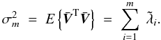 (16)We know that the
reconstructed signal only uses eigenprofiles of the signal subspace so that we can write
according to Eq. (11) their total energy
as,
(16)We know that the
reconstructed signal only uses eigenprofiles of the signal subspace so that we can write
according to Eq. (11) their total energy
as, 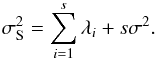 (17)The relative S/N of the
reconstructed signal can then be expressed as
(17)The relative S/N of the
reconstructed signal can then be expressed as 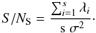 (18)On the other hand using
again Eq. (10) as well as Eq. (16) the energy of the original signal which
results from the signal subspace eigenvalues plus the noise contribution from the entire
m-dimensional domain is given by,
(18)On the other hand using
again Eq. (10) as well as Eq. (16) the energy of the original signal which
results from the signal subspace eigenvalues plus the noise contribution from the entire
m-dimensional domain is given by, 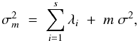 (19)and the relative S/N in
this case is
(19)and the relative S/N in
this case is 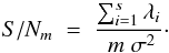 (20)This finally allows us to
write the gain factor g for the first stage of the SVD reconstruction,
(20)This finally allows us to
write the gain factor g for the first stage of the SVD reconstruction,
 (21)We see that due to
the projection of the observations onto the signal subspace we already obtain a signal
improvement of the order of m/s, i.e.
the noise level scales with
(21)We see that due to
the projection of the observations onto the signal subspace we already obtain a signal
improvement of the order of m/s, i.e.
the noise level scales with  .
The sample size also plays an import role in the reconstruction process and is relevant
for the noise level within the signal eigenprofiles as well as for the second stage of the
reconstruction process. Using Eq. (15)
together with the mean weighting scheme in the second stage and moreover realizing that
each subspace dimension contributes a total noise variance which is equal to the
eigenvalue σ2, the variance of the average of all subspace
dimensions then scales
with σ2/n.
.
The sample size also plays an import role in the reconstruction process and is relevant
for the noise level within the signal eigenprofiles as well as for the second stage of the
reconstruction process. Using Eq. (15)
together with the mean weighting scheme in the second stage and moreover realizing that
each subspace dimension contributes a total noise variance which is equal to the
eigenvalue σ2, the variance of the average of all subspace
dimensions then scales
with σ2/n.
However, let us again emphasize that our entire derivation above is based on an idealized noise behavior (i.e. wavelength independent white noise) which might be not fulfilled in real high-resolution spectroscopic observations. For a more reliable rank estimation as well as an estimation of the noise level for the reconstructed Stokes profiles, we will rely on a randomized bootstrap procedure (see next section).
3.2. Application to V410 Tau
To prepare the observation matrix ,
we first have to select a suitable number of Zeeman-sensitive spectral lines. This is done
by calculating a synthetic spectral atlas to judge which spectral line profiles are strong
enough and provide enough information.
By utilizing the forward module of iMap (Carroll et al. 2008) we synthesize Stokes I and Stokes V spectra for the observed wavelength range of our data (480–740 nm). The individual line parameters are taken from the VALD line list (Piskunov et al. 1995; Kupka et al. 1999). The astrophysical parameters for the synthetic calculations are those summarized in Sect. 4.4, except for the rotational velocity which is set to zero. A uniform temperature star with a homogeneous and purely radial surface magnetic field of 500 G is taken for the model spectra. The model atmospheres used throughout the analysis are Kurucz/Atlas-9 models (Castelli & Kurucz 2004).
The resulting synthetic spectral atlas (line list) in Stokes I and Stokes V is then used to select those spectral lines that fulfill the following criteria: Stokes I line depth ≥ 0.6 and Landé factor ≥ 1.5.
This procedure allowed us to select a list of 929 spectral lines. The majority of these
line are neutral Fe, Ca, Ti, Na, and C lines. For Stokes I, we only
select a short list of the strongest 56 iron lines because the intensity profiles are two
to three orders of magnitude larger than the polarized spectra. In this case there is no
need for a full reconstruction but instead a denoising
suffices, which requires a significantly smaller number of spectral lines. In a
first step, the observed spectra are transformed into velocity domain with a step size of
1.5 km s-1, which corresponds approximately to the lowest wavelength sampling
in the observed spectra. Then the line list is used to extract the corresponding
Stokes I and Stokes V profiles within a range of
± 150 km s-1 around their respective line centers. Using the extracted line
profiles, we then build the Stokes V observation matrix
and the Stokes I observation matrix
 as described in Sect. 3.
In total, 12 rotational phases were obtained within a time span of four weeks during
December 2008 and January 2009. For each of these 12 rotation phases, indexed with
p, we create an observation matrix
 and
and
 with 201
variables (intensities along the velocity domain) and a sample size of 929 for
and 56 for
. As described
in Sect. 3, a SVD provides us with the eigenvalues
and eigenprofiles of the observation covariance matrix from which we derive for each phase
a reconstructed average SVD profile.
with 201
variables (intensities along the velocity domain) and a sample size of 929 for
and 56 for
. As described
in Sect. 3, a SVD provides us with the eigenvalues
and eigenprofiles of the observation covariance matrix from which we derive for each phase
a reconstructed average SVD profile.
Because the original raw Stokes V spectra show no apparent sign of a
detectable line profile polarization, i.e. the polarimetric signals are much weaker than
the noise level, we adopt as an initial hypothesis that the observed
Stokes V spectra contain no signal information except
pure noise (not necessarily white). If this hypothesis is true then a random permutation
of the intensity values of each line across the velocity domain should not change the
outcome of our SVD analysis. In other words, if there are no systematic and coherent
features present among the spectral line profiles in the observation matrix, a random
scrambling of their individual wavelength or velocity binned intensity values would give
rise to the same series of eigenvalues. This series of ordered eigenvalues (ordered
according their magnitude) is called the eigenvalue spectrum. We therefore build a second
observation matrix for Stokes V where each extracted line profile is
subject to randomization across its velocity domain. If there are some sort of systematic
and coherent structures present in all observations the randomization process will
eliminate them such that the randomized covariance matrix provides essentially a flat
spectrum of eigenvalues, i.e. all eigenvalues  have the same
value
have the same
value  . Hence, in
the case where no significant systematic structures are present in the original
observation matrix the eigenvalue spectrum of the observation and randomized covariance
matrix will result in a flat eigenvalue spectrum within some error margin. On the other
hand if there are correlated and systematic features present we expect a distinct
difference in the eigenvalue spectrum.
. Hence, in
the case where no significant systematic structures are present in the original
observation matrix the eigenvalue spectrum of the observation and randomized covariance
matrix will result in a flat eigenvalue spectrum within some error margin. On the other
hand if there are correlated and systematic features present we expect a distinct
difference in the eigenvalue spectrum.
However, from random matrix theory it is known that a pure random matrix does not necessarily provide a flat eigenvalue spectrum and depend on the number of variables (wavelength) and measurements (spectral lines) (see e.g. Johnstone 2001). For this reason, we perform a Monte-Carlo simulation to provide a large sample (1000) of randomized covariance matrices from which we can deduce the mean eigenvalue spectrum and robust error margins for each eigenvalue. The errors of the eigenvalues are estimated by a bootstrap procedure (Efron & Tibshirani 1994) where we used again a sample size of 1000. After calculating the SVD of all the randomized matrices, we use a parallel analysis (Jolliffe 2002) to compare the significance of the eigenvalues of the observation covariance matrix relative to the mean eigenvalues (averaged over the respective subspace dimension) of all randomized covariance matrices.
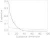 |
Fig. 1 Stokes V eigenvalue spectrum of a V410-Tau observation (solid line) and the mean eigenvalue spectrum obtained from a bootstrap randomization process (dashed line) for the first 100 dimensions of rotation phase 0.014. The magnitude of the eigenvalues of the corresponding observation covariance matrix and the mean eigenvalues of all randomized matrices are plotted over the corresponding subspace dimension index. The crossing point at dimension 27 marks the dimension from which on the individual eigenprofiles contain no more significant information. |
 |
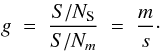
Fig. 2 Normalized Stokes I eigenvalue spectrum of the observation (solid line) and the noise variance (dashed line) for the first 20 subspace dimensions of rotation phase 0.014. For the purpose of a better illustration, the first three eigenvalues are not shown since they are significantly larger. The crossing point determines the signal subspace dimension to be 5. |
Note, that all matrices, the original observation matrix and each of the randomized
matrices, carry the same amount of total energy (variance), i.e. the total sum over all of
the eigenvalues are equal. After sorting the eigenprofiles for all covariance matrices
according to the magnitude of their respective eigenvalues, we can finally identify the
eigenprofiles of the observation covariance matrix that contain significant profile
information. This means we determine all those eigenprofiles whose
eigenvalues
are larger then the corresponding mean eigenvalues  of the randomized matrices.
This provides a noise threshold value according to Eq. (12) such that
of the randomized matrices.
This provides a noise threshold value according to Eq. (12) such that  which in turn
allows us to determine the effective rank of the signal subspace.
which in turn
allows us to determine the effective rank of the signal subspace.
Figure 1 shows the eigenvalue spectrum of the observation matrix and the mean eigenvalues from all the randomized matrices for one observational phase (0.014). The magnitude of the leading eigenvalues (solid line) obtained from the observation matrix provides a first evidence that the observation matrix contains significant information different from pure noise or random fluctuations which is indicated by the randomized eigenvalue spectrum (dashed line). The crossing point at which the eigenvalues from the observation covariance matrix drop below the eigenvalues of the randomized matrices marks the critical dimension in the subspace. Up to eigenvalue 27 the respective eigenprofiles contain significant information above the noise level. The estimated reduced rank is thus 27. This estimate allows us to proceed and use Eq. (15) to calculate the rank-reduced (subspace) averaged Stokes V profile. This procedure is then performed for all rotation phases to reconstruct the entire set of Stokes V profiles used in the following DI/ZDI inversion. Note that we omitted the error bars for both eigenvalue spectra in Fig. 1 because the standard deviation for all values is lower then 2% , which hardly exceeds the thickness of the plotted lines. For the Stokes I profiles, we have a significant larger relative S/N (it is in fact the S/N estimate from 2). Therefore, we do not start from a negative hypothesis that no signal or coherent information is present in the data set but instead directly apply Eq. (12) to determine the signal subspace. Figure 2 shows the normalized eigenspectrum for the first 20 eigenvalues of the observation covariance matrix (solid line) and the error variance σobs as determined from the observation (dashed line). It is interesting to see that almost the entire energy (variance) of the observation covariance matrix can be described by a very small number of eigenprofiles. The crossing point indicates that the subspace dimension is five. The first five eigenprofiles contain already 99.98% of the total energy of all line profiles within the observation matrix. In the following step, we again use Eq. (15) to calculate the subspace averaged Stokes I profiles.
Finally, Figs. 3 and 4 show the reconstructed set of Stokes V and Stokes I profiles for all rotational phases. The standard errors are provided again by a Bootstrap method with a re-sampling number of 1000. For each velocity bin, we thus obtained an estimate of the standard error which is condensed in Figs. 3 and 4 to a mean standard error value averaged over the velocity domain. Its typical value is 1 × 10⁻⁴ for Stokes V and 1 × 10⁻³ for Stokes I which corresponds to a signal-to-noise level of 10 000 or 1000 respectively.
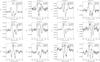 |
Fig. 3 Reconstructed SVD Stokes V profiles for each rotational phase of V410 Tau. Each profile is reconstructed from an observation matrix with a sample size of 929 spectral lines. The averaged standard error is given together with the corresponding rotational phase. |
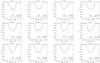 |
Fig. 4 Reconstructed SVD Stokes I profiles for each rotational phase. For all reconstructed profiles an observation matrix with 56 spectral lines is used. The averaged standard error is given together with the corresponding rotational phase. |
4. Stellar surface reconstruction with iMap
4.1. A brief description of iMap
In this study, we use the iMap code (Carroll et al. 2007, 2009) to simultaneously reproduce the temperature and magnetic vector field distribution from a sequence of observed Stokes I and V profiles. The forward modeling in iMap is based on polarized radiative transfer to allow for the best possible accuracy in line profile modeling (Carroll et al. 2009). All line parameters necessary for the synthetic calculation are taken from the Vienna atomic line list (VALD; Kupka et al. 1999. The underlying model atmospheres are based on Kurucz ATLAS-9 atmospheres (Castelli & Kurucz 2004). The actual calculation and integration of the polarized radiative transfer equation in LTE can be performed either by a numerical integration or by a number of trained artificial neural networks (ANN; Carroll et al. 2008).
The iMap code is equipped with a new inversion module. While the former versions relied on a conjugate gradient method (Press et al. 1992) with a local entropy regularization (Carroll et al. 2007), the current version of iMap uses an iteratively regularized Landweber method (Engl et al. 1996). Many different regularization methods exist for linear and non-linear inverse problems but interestingly only two of the most restrictive ones received attention in the field of ZDI and DI namely the Tikhonov regularization (see e.g. Piskunov & Kochukhov 2002) and the maximum entropy method (e.g. Vogt et al. 1987). There is also a long list of comparisons between these two methods and their benefits and respective shortcomings (see, e.g. Rice 2002). The three major issues that constitute an ill-posed, inverse problem are: (i) a solution may not exist; (ii) the problem may not be unique; (iii) the solution does not depend continuously on the data. We will not go into problem (i) which would require a discussion about the adequacy of the underlying ZDI/DI model assumptions (see Carroll et al. 2009, for a discussion), but instead we assume (as usual) that our model admits a solution. Then, we are left with the uniqueness problem (ii) and the numerical stability problem (iii) which both depend also on the noise level of the data. Problems (ii) as well as (iii) are closely related and can effectively be addressed by regularization methods that put additional constraints on the solution. Please also see in this context the paper of (Kochukhov & Piskunov 2002) who describes the degeneracy caused by using just the information of the Stokes I and Stokes V profiles. In our iterative approach, implemented in iMap, problem (ii) and (iii) will be addressed by an iteration process where the step size and an appropriate stopping rule provide the regularization of the inverse problem (Engl et al. 1996).
Iterative regularization for inverse problems has been the subject of various theoretical
investigations over the recent years (Hanke 1997;
Engl & Kugler 2004; Egger & Neubauer 2005; Kaltenbacher et al. 2008). The Landweber iteration, which is used here, rests on
the idea of a simple fixed-point iteration, derived from minimizing the sum of the squared
errors. Our new inversion routine follows exactly this line and can be described as
follows: written in a concise vector notation the problem setting is 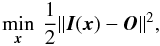 (22)where ∥ ∥ is the
L2 norm and I is the synthetic
model profile over all spectral lines, wavelengths or velocities, and rotational phases,
O is the corresponding observation. The vector
x contains all our free parameters of the model, i.e.
the temperature and the magnetic field vector for each surface element. The iteration now
proceeds along the negative gradient direction and updates the current estimate of the
solution vector, xk, in the
following manner
(22)where ∥ ∥ is the
L2 norm and I is the synthetic
model profile over all spectral lines, wavelengths or velocities, and rotational phases,
O is the corresponding observation. The vector
x contains all our free parameters of the model, i.e.
the temperature and the magnetic field vector for each surface element. The iteration now
proceeds along the negative gradient direction and updates the current estimate of the
solution vector, xk, in the
following manner  (23)Here,
I′ is the gradient
vector with respect to all surface element values and
wk is the weight factor that can
adaptively accelerate the iteration process. In the conventional Landweber iteration
process, wk is set to unity. To accelerate
the procedure we use a variant of the steepest descent (Kaltenbacher et al. 2008) and
set wk to
(23)Here,
I′ is the gradient
vector with respect to all surface element values and
wk is the weight factor that can
adaptively accelerate the iteration process. In the conventional Landweber iteration
process, wk is set to unity. To accelerate
the procedure we use a variant of the steepest descent (Kaltenbacher et al. 2008) and
set wk to 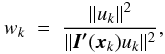 (24)where
uk = I′ ∗ (O−I(xk)).
(24)where
uk = I′ ∗ (O−I(xk)).
The semi-convergence (Hanke et al. 1995) of the
method requires a stopping rule before it enters into the noise level of the data to
regularize the procedure and to avoid overfitting. One common, and well studied criterion
for the stopping condition is the Morozov discrepancy principle which can be written for
the iterative approach as  (25)where δ
is an upper bound for the data error (i.e. noise), τ a positive number
and k ∗ the maximum iteration number. In terms of stability
and convergence it can be shown that τ has to
satisfy τ ≥ 1 (Engl et al. 1996).
Formally the noise estimate for the ZDI/DI can be derived from the observations. Given a
noise contribution σi for each
velocity i we can combine the individual errors to form a vector
σ such as,
σT = (σ1,σ2,...,σn)
with n the number of velocity points. The error can then be expressed as
δ = ∥ σ ∥ . If the noise estimate is
homogeneous (i.e. equal for all velocities) or does not vary much over the velocity domain
and time we may use the maximum of σ to write for
δ the relation
(25)where δ
is an upper bound for the data error (i.e. noise), τ a positive number
and k ∗ the maximum iteration number. In terms of stability
and convergence it can be shown that τ has to
satisfy τ ≥ 1 (Engl et al. 1996).
Formally the noise estimate for the ZDI/DI can be derived from the observations. Given a
noise contribution σi for each
velocity i we can combine the individual errors to form a vector
σ such as,
σT = (σ1,σ2,...,σn)
with n the number of velocity points. The error can then be expressed as
δ = ∥ σ ∥ . If the noise estimate is
homogeneous (i.e. equal for all velocities) or does not vary much over the velocity domain
and time we may use the maximum of σ to write for
δ the relation 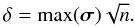 (26)If we assume that
Eq. (22) follows a
χ2 distribution we may use the number of degrees-of-freedom
of the problem to determine the error resulting from the limited degree of freedom of the
model to write
(26)If we assume that
Eq. (22) follows a
χ2 distribution we may use the number of degrees-of-freedom
of the problem to determine the error resulting from the limited degree of freedom of the
model to write 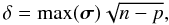 (27)where p
is the number of parameters in the model. If the inversion reduces the error function
Eq. (22) down to the threshold
δ we would ensure that the reduced χ2 is
close to one. But let us emphasize here that DI as well as ZDI (given we have correctly
modeled the problem) are non-linear problems (see Carroll
et al. 2009) and moreover the problem is generally ill-posed, which makes it by
no means a simple task to adequately determine the real degree of freedom of the problem.
The reduced χ2 as a measure of the goodness-of-fit
may therefore only of limited use.
(27)where p
is the number of parameters in the model. If the inversion reduces the error function
Eq. (22) down to the threshold
δ we would ensure that the reduced χ2 is
close to one. But let us emphasize here that DI as well as ZDI (given we have correctly
modeled the problem) are non-linear problems (see Carroll
et al. 2009) and moreover the problem is generally ill-posed, which makes it by
no means a simple task to adequately determine the real degree of freedom of the problem.
The reduced χ2 as a measure of the goodness-of-fit
may therefore only of limited use.
If the data are pre-processed like in this work the noise estimate for the SVD reconstructed data can be directly obtained from the error estimates provided by the bootstrap procedure given in the last section.
The simultaneous DI and ZDI procedure for each surface element, is implemented in the
following way. Instead of using one long vector x that
incorporates the entire information of the surface temperature and the magnetic field, we
proceed with an alternate minimization (Byrne 2004)
of Eq. (22). Alternate minimization means
here that after each iteration for the temperature  a parallel inversion of the magnetic field vector
xB is performed, which uses the information of
the k + 1 iteration of the temperature minimization. The alternate
iteration at step k + 1 for
and
a parallel inversion of the magnetic field vector
xB is performed, which uses the information of
the k + 1 iteration of the temperature minimization. The alternate
iteration at step k + 1 for
and  can then be written as
 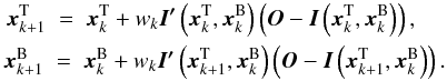 (28)Note
that both
and
depend on each other due to radiative transfer effects.
(28)Note
that both
and
depend on each other due to radiative transfer effects.
We want to note here that after a careful analysis of the convergence and stability behavior of the inversion, the strict simultaneity of the temperature and magnetic inversion is not necessarily required whereas the order of the inversion is of importance. The dependence of the DI on the magnetic inversion is not strong, this is mainly due to the weakness of the effect that the magnetic field introduces via the Zeeman effect on the intensity profile (Stokes I). For rapid rotating cool stars the temperature information encoded in line profile bumps of the Stokes I profiles is therefore only weakly affected. The dependence of ZDI on the temperature inversion however is strong, which means the temperature information obtained from the DI must be part of the magnetic inversion as the temperature leads to a non-trivial scaling of the Stokes V profile amplitude and width. A consecutive DI-ZDI approach is therefore equivalent to the simultaneous inversion as done in this work.
4.2. Multi-line inversion
For DI as well as for ZDI we could apply the least-squares minimization of Eq. (22) to all of our available and reconstructed
spectral lines simultaneously, i.e. using a combined long spectral line vector such that
the error function reads 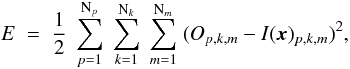 (29)where
x is the model parameter vector, p the
rotational phase, k the spectral line, m the wavelength
or the velocity index respectively, and Np,
Nk, Nm their respective total
numbers. This is the approach usually pursued in DI with TempMap (e.g.
Rice & Strassmeier 2000; Rice et al. 2011) but fails for ZDI since the
polarimetric signals are usually buried deep within the noise and therefore require a
signal extraction which provides a reconstructed composite line profile. The SVD
reconstruction process extracts a single (weighted) mean SVD line profile that comprises
the information of all the contributing lines of the observation matrix and therefore the
error function can no longer be applied to the sum of squared differences of the
individual lines but needs to be applied on the squared differences between the
reconstructed SVD profile and a proper synthetic equivalent. The strategy here is in fact
to compute a synthetic mean profile for all contributing spectral lines used in the SVD
reconstruction process by accounting for all radiative transfer effects and line modeling
characteristics (e.g. model atmospheres, spectral line parameters and line blends).
(29)where
x is the model parameter vector, p the
rotational phase, k the spectral line, m the wavelength
or the velocity index respectively, and Np,
Nk, Nm their respective total
numbers. This is the approach usually pursued in DI with TempMap (e.g.
Rice & Strassmeier 2000; Rice et al. 2011) but fails for ZDI since the
polarimetric signals are usually buried deep within the noise and therefore require a
signal extraction which provides a reconstructed composite line profile. The SVD
reconstruction process extracts a single (weighted) mean SVD line profile that comprises
the information of all the contributing lines of the observation matrix and therefore the
error function can no longer be applied to the sum of squared differences of the
individual lines but needs to be applied on the squared differences between the
reconstructed SVD profile and a proper synthetic equivalent. The strategy here is in fact
to compute a synthetic mean profile for all contributing spectral lines used in the SVD
reconstruction process by accounting for all radiative transfer effects and line modeling
characteristics (e.g. model atmospheres, spectral line parameters and line blends).
We briefly show that the result of this strategy provides an error which is on average at
least as low as in the conventional case, where the sum of differences from each
contributing line is computed according Eq. (22). Let us begin with the conventional case of Eq. (29). For brevity we incorporate the rotational
phases and the wavelengths or velocities into the vector notation such that
Ik and
Ok represent the Stokes
profile of one particular spectral line k taken over the entire velocity
range and over all available rotational phases. If we correctly model each individual
spectral line that contributes to the averaging process, then we can express the
difference between the observed Stokes profile
Ok and the synthetic profile
Ik as being exclusively due
to the inherent noise ϵk such
that Ik corresponds to the
observation Ok within the
limits of ϵk;  (30)The average
sum-of-squares error for a particular line profile can then be written as
(30)The average
sum-of-squares error for a particular line profile can then be written as ![Mathematical equation: \begin{equation} E_k \; = \; \mathcal{E} \left[ (\vec{I}_{k} - \vec{O}_{k})^2 \right] \; = \; \mathcal{E} \left[\vec{\epsilon}_k^2 \right], \label{Eq:4_7} \end{equation}](/articles/aa/full_html/2012/12/aa20215-12/aa20215-12-eq122.png) (31)The mean error
(31)The mean error
 of all individual spectral lines is then given as
 ![Mathematical equation: \begin{equation} \tilde{E} \; = \; \frac{1}{{\rm N}_k} \; \sum_{k=1}^{{\rm N}_k} E_k \; = \; \frac{1}{{\rm N}_k} \; \sum_{k=1}^{{\rm N}_k} \mathcal{E} \left[ \vec{\epsilon}_k^2 \right]. \label{Eq:4_8} \end{equation}](/articles/aa/full_html/2012/12/aa20215-12/aa20215-12-eq124.png) (32)On the other hand, if we
perform the averaging process before minimizing the error function, as we did in our line
profile extractions, we can write for the mean observed profile pattern
(32)On the other hand, if we
perform the averaging process before minimizing the error function, as we did in our line
profile extractions, we can write for the mean observed profile pattern  (33)and the same holds for
the mean synthetically calculated profile
(33)and the same holds for
the mean synthetically calculated profile  (34)The mean error
 for the pre-averaged line profile can then be written as
 ![Mathematical equation: \begin{equation} \bar{E} \; = \; \mathcal{E} \left[ \left( \frac{1}{{\rm N}_k} \; \sum_{k=1}^{{\rm N}_k} ( \vec{I}_k - \vec{O}_k ) \right)^2 \right]. \label{Eq:4_11} \end{equation}](/articles/aa/full_html/2012/12/aa20215-12/aa20215-12-eq128.png) (35)This is equivalent
to
(35)This is equivalent
to ![Mathematical equation: \begin{equation} \bar{E} = \mathcal{E} \left[ \left( \frac{1}{{\rm N}_k} \; \sum_{k=1}^{{\rm N}_k} \vec{\epsilon}_k \right)^2 \right]. \label{Eq:4_12} \end{equation}](/articles/aa/full_html/2012/12/aa20215-12/aa20215-12-eq129.png) (36)We are assuming again
that the noise ϵk is
uncorrelated and of zero mean, so that all covariance terms disappear. Then we may write
(36)We are assuming again
that the noise ϵk is
uncorrelated and of zero mean, so that all covariance terms disappear. Then we may write
![Mathematical equation: \begin{equation} \bar{E} = \frac{1}{{\rm N}_k^2} \; \sum_{k=1}^{{\rm N}_k} \; \mathcal{E} \left[ \vec{\epsilon}_k^2 \right]. \label{Eq:4_13} \end{equation}](/articles/aa/full_html/2012/12/aa20215-12/aa20215-12-eq130.png) (37)Comparing this with
Eq. (32) shows immediately that the mean
error for the averaged line profile is lower than for the individual profiles,
(37)Comparing this with
Eq. (32) shows immediately that the mean
error for the averaged line profile is lower than for the individual profiles,
![Mathematical equation: \begin{equation} \bar{E} \; = \; \frac{1}{{\rm N}_k^2} \; \sum_{k=1}^{{\rm N}_k} \; \mathcal{E} \left[ \vec{\epsilon}_k^2 \right] \; \leq \; \frac{1}{{\rm N}_k} \; \sum_{k=1}^{{\rm N}_k} \mathcal{E} \left[ \vec{\epsilon}_k^2 \right] \; = \; \tilde{E}. \label{Eq:4_14} \end{equation}](/articles/aa/full_html/2012/12/aa20215-12/aa20215-12-eq131.png) (38)Most likely, the
idealized assumption of completely uncorrelated noise is not valid but still, the error of
the averaged modeling
is not expected to be larger than that of a conventional minimization of
.
Note, that an important aspect here is the correct synthetic modeling of the averaged
profile. The extension to a weighted averaging is straight forward.
(38)Most likely, the
idealized assumption of completely uncorrelated noise is not valid but still, the error of
the averaged modeling
is not expected to be larger than that of a conventional minimization of
.
Note, that an important aspect here is the correct synthetic modeling of the averaged
profile. The extension to a weighted averaging is straight forward.
4.3. Differential rotation inversion
In this section, we introduce our methodology for retrieving a surface differential rotation signal, if present. Our technique follows closely that introduced by Petit et al. (2002). Given that the observations span over several rotational phases and that the stellar surface obeys a solar-type differential rotation law, the underlying idea is that the closer the modeled differential rotation is to the true value the lesser the resulting reconstructed surface image is smeared out. In other words, not accounting for differential rotation introduces a blurring effect in the resulting DI or ZDI. Differential rotation provides not only constraints on the image space in terms of the resulting sharpness of the image but also on the data space because the differential rotation alters the velocity distribution of the individual local line profiles over the visible surface and thus produces a modification of the disk-integrated flux profile (see, e.g. Gray 2005). The data space approach has been extensively used in the past for determining the differential rotation of a number of stars (e.g. Reiners & Schmitt 2003; Reiners 2006). Compared to the approach chosen by Petit et al. (2002) and Donati et al. (2003) there is one major difference we apply here. Instead of repeating the inversion many times with various differential rotation parameters to sample the χ2 landscape, we directly incorporate the differential rotation law into the inversion. All other restrictions given in Sect. 5.1 of Petit et al. (2002) also hold for our approach with particular emphasis on the required rotational coverage, note that the requirements for the phase coverage is less restrictive.
4.3.1. Assumed differential-rotation law
The assumption here is that the differential rotation on V410 Tau can be described, as
for so many cool and late-type stars, with a simplified “solar-type” differential
rotation law;  (39)where
l is the surface latitude, Ω(l) the respective rotation rate at a
particular latitude, Ωeq the rotation rate at the equator, and dΩ the
difference in rotation rate between the pole and the equator.
(39)where
l is the surface latitude, Ω(l) the respective rotation rate at a
particular latitude, Ωeq the rotation rate at the equator, and dΩ the
difference in rotation rate between the pole and the equator.
4.3.2. Implementation as a sheared-image analysis within iMap
The search for the least blurred image consistent with the minimum of the objective
Eq. (22) can also be expressed as an
image deconvolution problem with a latitudinal smearing operator or point-spread
function Plat. This concept will be investigated and
developed in a future paper, instead we concentrate here on describing the problem in
the same way as in Petit et al. (2002). Providing
sharpness as an additional constraint in image space may indeed provide a means of
finding a solution which best matches with a differential rotation law and the data
error (fit) at the same time. This extra constraint has been provided in terms of
minimizing the information content (maximizing the image entropy) of the image by Donati et al. (2000) and Petit et al. (2002). However, because maximum entropy is entirely
invariant under a random permutation of the image data (pixel) and does not account for
any spatial coherence in the image domain, we believe this constraint is not an
appropriate measure to quantify distortions due to surface differential rotation.
Moreover differential rotation may, despite the distortions, retain to a large extent
the morphological coherency of surface structures over several rotation periods. Instead
of adding an additional constraint to the error function, we want to completely rely on
the achieved quality of the data fit and implement the optimization for the two
parameters Ωeq and dΩ within the iMap code. This extra
flexibility amounts to an additional degree of freedom in the time domain to account for
the time-dependent rotational evolution of the image. The profiles and the corresponding
part of the visible stellar disk are no longer only determined just by the spectral
information of the respective phase alone but also by the time information (Petit et al. 2002). This minimization process can
conveniently be incorporated into our Landweber iteration in Eq. (28) to yield an alternating minimization
scheme. If we define the vector Ω which comprises our two
differential rotation parameter Ωeq and dΩ the process can be described as
follows: after proceeding along the negative gradient direction in image space
(temperature and/or magnetic field) the process switches to the omega space to perform a
minimization of the squared error, Eq. (22) with respect to the differential parameter vector
Ω. This provides a new current estimate of the vector
Ω. which then enters again in the next iteration cycle of
Eq. (28) This process is repeated
until the stopping condition is reached (see Sect. 4). We can formally introduce an image-shear operator
Pd which differentially rotates a current estimate
xk(Ω)
of the image (temperature or magnetic field) to write the process as ![Mathematical equation: \begin{equation} \hat{\vec{\Omega}} \; = \; \arg\min_{\vec{\Omega}} \;\mathbb{P}_d \; \left [ \vec{x}_k(\vec{\Omega}) + w_k \vec{I'}(\vec{x}_k(\vec{\Omega})) \left ( \vec{O} - \vec{I}(\vec{x}_k(\vec{\Omega})) \right ) \right ]. \label{Eq:4_16} \end{equation}](/articles/aa/full_html/2012/12/aa20215-12/aa20215-12-eq141.png) (40)The minimization of
Eq. (40) is performed by a gradient
descent method similar to the one used for the Landweber iteration.
(40)The minimization of
Eq. (40) is performed by a gradient
descent method similar to the one used for the Landweber iteration.
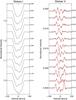 |
Fig. 5 Stacked plot of the synthetic fits (thick dashed lines) to the observed Stokes profiles (thin solid lines), on the left side Stokes I and on the right Stokes V. All spectral line profiles are normalized by the continuum intensity. |
 |
Fig. 6a Orthographic maps of the temperature distribution of V410 Tau at four different rotational phases φ. |
 |
Fig. 6b Orthographic maps of the magnetic field distribution of V410 Tau at four different rotational phases φ. The magnetic field is color coded and the field lines are proportional to the field strength (blue negative and red positive polarity). |
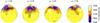 |
Fig. 6c Orthographic maps of the temperature overplotted by the magnetic field lines at four different rotational phases φ. For a better visibility the positive fields are color coded in yellow while the negative fields are again in blue. As above the field lines are proportional to the strength of the field. |
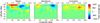 |
Fig. 7 Pseudo-Mercator projection of the three magnetic-field components; left radial, middle meridional, and right azimuthal. Note, that the lower x-axis is the longitudinal angle, while the upper x-axis gives the rotational phase. The dotted line indicates the limit for the visibility due to the stellar inclination. |
4.4. Fixed stellar parameters
The adopted stellar parameters are the same as those used and partly derived in Paper I. The effective temperature is 4400 K, the logarithmic gravity is 4.0, the projected rotational velocity is 77.7 km s-1, and the inclination of the stellar rotation axis is 62° as determined from DI in Paper I. The micro- and macro-turbulence is set to 2.0 km s-1 and 1.5 km s-1, respectively, solar chemical abundances are assumed for all elements. As also described in detail in Paper I, an average rotational period of 1.871948 d was adopted. Rotational phase is also kept the same as in Paper I.
4.5. iMap setup
For the inversion with iMap, we use all 12 available Stokes I and Stokes V SVD profiles from Figs. 3 and 4. We utilize the multi-line approach described in Sect. 4.2 which requires to synthesize all 929 spectral line profiles of the observation matrix to finally obtain the mean synthesized profile. The enormous amount of computation is performed by our ANN approach (Carroll et al. 2008). As mentioned in Sect. 4.1 all line parameters were taken from the VALD line list and model atmospheres are produced by ATLAS-9 (Castelli & Kurucz 2004). The stellar surface is partitioned into 6° × 6° segments, whereas the polarized radiative transfer is calculated on a subpartition of 3° × 3°. The initialization temperature was homogeneously set to 4400 K. The initial magnetic field is homogeneously set to zero for all three magnetic components (radial, azimuthal and meridional). For vsini, stellar inclination, gravity, and abundances, the values given in Sect. 4.4 are used.
The stopping rule according to the discrepancy principle for the Landweber iteration is set according to the standard errors of the reconstructed line profiles. As described in Sect. 4.1 this means that we use for the magnetic inversion the largest (maximum) standard error of the reconstructed Stokes V profiles and for the temperature inversion the largest standard error of the reconstructed Stokes I profiles. The individual values are shown in Figs. 3 and 4.
5. Application to V410 Tau
5.1. Temperature distribution in 2008/09
The synthetic fits relative to the observed Stokes I profiles are shown in a stacked plot on the left side of Fig. 5. The final temperature map in orthographic projection is shown in Fig. 6a. It is dominated by a structured, cool, polar cap with a temperature as cool as ≈ 3500 K, i.e. ≈ 900 K below the effective temperature. Several appendages reach down to lower latitudes of around 30° with decreasing temperature contrast the further they are away from the cap. The total spot filling factor is 11.9%. From previous investigations, we knew that V410 Tau shows a polar spot and a number of smaller cool spots together with localized hot features (see the review in Paper I). However, the simultaneous reconstruction of the surface temperature and the magnetic-field distribution provides unprecedented accurate surface details.
An interesting feature of the temperature map in Fig. 6a is the pair of isolated spots consisting of a cool spot at phase φ ≈ 0.7 and of a hot spot at phase φ ≈ 0.6 at intermediate latitudes. The hot spot’s temperature is ≈ 4800 K, i.e. ≈ 400 K above the effective temperature while the cool spot’s temperature is ≈ 4000 K, i.e. ≈ 400 K below the effective temperature. A similar pair of spots, although larger in size and with much smaller contrast, is located on the equator at phase φ ≈ 0.25. This pair’s temperature difference is ≈ 400 K in total. Yet a third such pair of just moderate warm and cool spots may exist around φ ≈ 0.0 at latitude ≈ 30°.
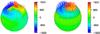 |
Fig. 8 Intriguing structural similarity between the result of our magnetic surface reconstruction (left) and an α2Ω-dynamo simulation which is scaled to a surface field strength of 1.9 kG (right). |
All of above features were independently reconstructed with TempMap and iMap in Paper I; some with slightly different contrast but the overall similarity is very good.
5.2. Magnetic field distribution in 2008/09
The magnetic field reconstruction found by iMap provides a solution compatible with the observed data and the noise level. The synthetic fits for the individual Stokes V profiles are shown in a stacked plot in Fig. 5. The ZDI map is shown as an orthographic plot in Fig. 6b. The distribution of the individual magnetic components (radial, azimuthal and meridional) can be best seen in the pseudo Mercator-projection plot in Fig. 7. The orientations of the field within the Mercator plots is defined such that a positive direction in the radial field points outward while a negative polarity points inward, the meridional component is positive if it points toward the upper north-pole and negative in the direction of the south-pole. For the azimuthal component a positive field is defined in westward direction and negative for an eastward direction.
The magnetic topology on V410 Tau is dominated by a bipolar structure around the visible pole with peak field strengths of up to ± 1.9 kG. Figure 6c emphasizes the relatively good correlation of the temperature and magnetic field and shows that the strongest fields are located in the darkest regions around the pole. The two polarities appear separated by a sharp, pole-crossing, neutral sheet. In total the field forms an S-shaped structure centered at the rotation pole. The topology is predominantly radial but 1 kG meridional components coexist very close to the pole. An azimuthal component, on the other hand, is restricted to a region at ≈ 60°-latitude and around 270° longitude, i.e. 180° away from the strongest radial component, close in distance but on the opposite hemisphere and always of positive polarity. Its peak field strength reaches 1 kG around 270° longitude while the rest of it mostly remains near 500 G. One can express the field topology also in terms of the poloidal and toroidal components which reveals in our case that the majority, 73%, of the surface field of V410 Tau is given in the form of poloidal fields and just 27% being in form of a toroidal component.
The dominant of the two isolated warm-cool spot pairs around φ ≈ 0.6 and φ ≈ 0.7 has no recognizable distinct magnetic-field structure. Both, the cool and the warm spot, appear with the same general mix of field components as their immediate surrounding and at least this particular spot pair is reconstructed with the same (positive) polarity. On the contrary, the second such spot pairs (around φ ≈ 0.25; see Sect. 5.1 above) indicates a mixed polarity, negative for the warm feature and positive for the cool feature.
It is interesting to note that the strong Hα flare reported in Paper I (located at φ ≈ 0.18) coincides with the best visibility of the sharp neutral sheet of the bi-polar radial field. It is at least tempting to state that, if truly coincident, it would very well agree with solar active-region physics where flares are usually related to the current sheets separating opposite polarities (e.g. Schrijver et al. 2005).
An error analysis of the here presented results is given in the Appendices A–C.
5.3. Differential rotation of V410 Tau
As described in Sect. 4.3 a solar like differential rotation parameterized by Ωeq and dΩ is part of the inversion process. In the current version of iMap the sheared image analysis is applied to the temperature structures only. For the initialization, Ωeq is derived from the rotational period of 1.871948 d (see Paper I). Only a very weak solar-like differential rotation is present, if at all. The formal value for the angular velocity at the equator is Ωeq = 3.356 ± 0.005, well within the errors of the photometrically determined rotation period, and for the differential rotation rate between the equator and the pole we have dΩ = 0.007 ± 0.009. We can not safely regard this as a detection of a differential rotation on V410 Tau but conclude that it must be very small, likely smaller than a factor 30 compared to the Sun.
5.4. The magnetic nature of V410 Tau
The probable absence of a radiative core and the non-detection of differential rotation in this work and other investigations (Strassmeier et al. 1994; Skelly et al. 2010) leaves not much room for speculation about the nature of the dynamo operating in the interior of V410 Tau – at least in the framework of classical mean field dynamos. As has been shown by Küker & Rüdiger (1999) a likely explanation for the generation of the magnetic field in WTTS can be given in terms of a α2-dynamo.
From the observational point of view we can characterize and quantify the surface topology with various degrees of detail but providing a quantitative link between observation and theory is anything but straightforward. In the moment we feel that dynamo theory does not give enough reliable information to provide such a quantitative link between the surface appearance of magnetic fields and their internal generation process. But this shall not keep us from giving qualitative arguments in favor of an α2-dynamo here. Following Küker & Rüdiger (1999) for an α2-dynamo the field topology exhibit a distinct non-axisymmetric geometry with S1- or A1-type modes (Rüdiger & Hollerbach 2004). The pronounced bipolar magnetic field at the pole (Fig. 6b) can easily be identified with such a non-axisymmetric geometry. However the fact that the non-axisymmetric mode of such an α2-dynamo solution can only rotate with the star itself (except for a slight drift) may not really fit to recent observations that V410 Tau exhibit a periodic change of its activity in the range between 4.8 to 5.5 years (Stelzer et al. 2003; Savanov 2012). But a possible explanation can still be given in terms of an α2Ω-dynamo (Elstner & Korhonen 2005), where the non-axisymmetric solution is modulated by an oscillatory axisymmetric mode. The excitation of such an α2Ω-dynamo can already occur at a very low differential rotation rate (Elstner & Korhonen 2005). To qualitatively compare this dynamo model with our reconstructions we have taken a snapshot of the non-axisymmetric mode of these simulations at a time when both magnetic polarities are of approximately the same strength. The surface field strength was scaled to be comparable to that of the reconstructed surface field of V410 Tau and the symmetric field (relative to the equator) at the south pole has been damped. The similarity between our reconstruction and the α2Ω-dynamo simulation shown in Fig. 8 is quite remarkable and may in fact strengthen the hypothesis that the field of weak-lined T Tauri stars is generated by an α2-type dynamo or in cases where a weak differential rotation has already developed by an α2Ω-dynamo.
An interesting model which accounts for the evolution of pre-main sequence dynamos were presented by Kitchatinov et al. (2001) and may also be applicable to our findings. According to their simulations the dynamo during the early phases of the pre-main sequence stage, when the core development is still in progress and the rotational velocity is large, gives rise to a strong non-axisymmetric mode. In the course of the evolution when differential rotation sets in the star develops an increasing axisymmetric dynamo mode which can lead to an oscillating behavior (Rüdiger & Elstner 1994) before the field is eventually completely dominated by the axisymmetric mode at a later stage.
How does V410 Tau compares with other T Tauri stars that have been subject to magnetic investigations. Zeeman-Doppler-Imaging has been applied to a small number of classical T Tauri stars and have been compared by Hussain (2012) to find a relation between mass, period, magnetic field strength and field complexity. Although no clear relation could be found from the limited sample, there seems to be a tendency that fully convective T Tauri stars may harbor simpler surface fields (i.e. mainly a dipole pole component) while T Tauri stars which have developed a radiative core have the tendency to more complex fields Hussain (2012). It is not clear if V410 Tau as a weak-lined T Tauri fit into this picture. Given its evolutionary stage it may be reasonable to assume, in the light of the above trend, that V410 Tau exhibit a more complex surface field than just a dipole (spherical harmonic numbers l = 1 and m = 0). This is in fact true, but our magnetic reconstruction shows just a little more additional complexity with a clear dominance of the S1 mode (l = 1,m = 1) and the A1 mode (l = 2,m = 1). The apparent diversity of the magnetic field of T Tauri stars certainly requires a greater sample in order to provide a more general picture of the magnetic evolution and the underlying dynamo for these pre-main sequence stars.
At the end we also want to comment on the apparent differences between the reconstructed surface fields of Skelly et al. (2010) and our magnetic and temperature maps. In a recent magnetic investigation of V410 Tau Skelly et al. (2010) found that 50% of the total field has a toroidal component and the other 50% are poloidal and that the majority of the field shows strongly inclined large-scale azimuthal fields which are distributed over one entire hemisphere, whereas our reconstructed topology has only 27% toroidal fields and 73% poloidal fields with a strong radial and bipolar component around the polar region. Moreover, in contrast to our reconstructed maps where the strong magnetic fields are well correlated with the temperature, see Fig. 6c, the fields of Skelly et al. (2010) seem to show almost no correlation with their brightness maps (i.e. a proxy of the temperature distribution). The fact that these data were observed at almost the same time as ours (January 2 to January 17, 2009) at the Telescope Bernard Lyotl (TBL) with the NARVAL spectropolarimeter at the Pic di Midi, is certainly a reason for a closer inspection and comparison of the two results. Without having the possibility for doing such a detailed comparison of the data as well as of the inversion codes we can only speculate about the reasons for the disparity of the two reconstructions. But we want to emphasize that in contrast to Skelly et al. (2010) our approach makes no assumptions on the surface topology in terms of a spherical harmonic decomposition or potential field structure. It is furthermore fully based on polarized radiative transfer and line profile modeling and it pursues a strategy which simultaneously invert the temperature and magnetic field. This give us enough confidence to believe in the validity of our results.
6. Summary and conclusions
Despite the relative high levels of magnetic activity of many rapidly rotating late-type stars the typical spectropolarimetric signals that these stars produce are mostly below the noise level of a typical spectropolarimetric observation and require therefore specialized techniques to extract and reconstruct the line profiles. To address this problem we have developed a new SVD based spectral-line extraction technique. For Stokes V this approach is a full reconstruction method which allows us in this work to reach an improvement in the S/N by a factor of 40. For Stokes I where the actual signals are orders of magnitudes larger then for Stokes V the SVD method reduces to a denoising technique but still allows to increase the signal-to-noise ratio by a factor of 5.
The interpretation of polarimetric data in terms of ZDI always require the introduction of additional information. This is true for the underlying model used in the inverse problem as well as for the regularization of the problem itself. To pose a minimum number of surface constraints on the solution we have chosen a new regularization approach for DI and ZDI in terms of an iterative regularization of the problem. The new variant implemented in the inverse module of iMap shows a good and stable behavior and converges within 400 iterations.
A common problem for ZDI is that the real strong magnetic fields which are associated with cool surface regions produce only a fraction of the photon flux compared to the unaffected quiet or even hot surface regions. To prevent our code from these ill-defined flux-weighting and the mutual effects between the temperature and magnetic fields we have pursued a strategy that performs a simultaneous DI and ZDI to retrieve both the temperature and the magnetic field distribution at the same time.
The reconstruction of the temperature and magnetic field of V410 Tau reveals that the majority of the strong fields of 2 kG are located in the cool spots, in particular within the large polar spot. The reconstruction clearly show that both polarities coexist within the large polar spot and that the entire polar-field topology appears to be dominated by a twisted bi-polar structure separated by a relatively sharp neutral line. It is reminiscent of an over-dimensioned solar active region. Even the time of a strong flare coincides with the best visibility of this neutral line, just like for solar active regions. However, due to its shear size of approximately 11% of a hemisphere, the bi-polar feature appears S-shaped as if it had been dragged around the pole due to the rapid stellar rotation. The absence of a detectable differential rotation and the pronounced non-axisymmetry of the field may suggest an α2-dynamo operating in the interior of V410 Tau. This is also supported by the intriguing similarity between our reconstructed surface fields and the dynamo simulation of Elstner & Korhonen (2005), and may support the theory that the underlying mechanism responsible for the magnetic field generation in weak-line T Tauri stars is an α2-type dynamo.
Online material
Appendix A: Error analysis
 |
Fig. A1a Temperature error map in orthographic projection at four different rotational phases. The maximum rms value is 80 K and the mean rms value is 50 K. Regions below a latitude of –30° are set to a constant value and do not participate in the error estimation. |
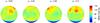 |
Fig. A1b Radial magnetic field error map in orthographic projection at four rotational phases, the maximum rms value is 125 G and the mean rms value is 64 G. |
In this section, we want to investigate the significance of our reconstruction results, in particular we want to quantify how sensitive the solution of the inverse problem is with respect to the initial conditions. In our DI and ZDI setup we deal with four parameter spaces (temperature, radial magnetic field, azimuthal magnetic field and meridional magnetic field) each of which with a dimension equal to the number of surface segments. The inversion algorithm has to navigate through the combined parameter spaces to find a solution that is compatible with the data. To study the stability of the inversion relative to the initial starting conditions (different positions in the parameter spaces) we use a simulation that runs the inversion with the original data set but from randomly chosen starting positions. Each parameter space is independently initialized by choosing a random value for each surface segment. Though we may create a considerable spread among the individual surface segments we can only consider a small fraction of the overall parameter space. Any exhaustive study to sample the parameter space is way out of reach for this high-dimensional setting and it is not the purpose here, instead we want to gain a quantitative measure how the result varies when the initial conditions are changed.
 |
Fig. A1c Meridional magnetic field error in orthographic projection, the maximum rms value here is 101 G and the mean rms value is 51 G. |
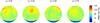 |
Fig. A1d Azimuthal magnetic field error in orthographic projection with a maximum rms value of 106 G and a mean value of 52 G. |
A random generator on the basis of a normal distribution provides the values for each parameter space and surface segment. The underlying normal distribution has a mean value which is set to the effective temperature for the temperature component and to zero Gauss for all three magnetic components. The standard deviation is 250 K for the temperature and 250 G for all the magnetic components to provide a large spread among the individual surface segment values. The simulation (inversion with different initializations for all parameters and segments) is runfor 100 times on the original data set. For the so obtained 100 DI and ZDI maps we calculated the root-mean-square (rms) error to finally get rms error maps for each parameter. The individual inversions are all run to the same accuracy level given by the noise of the reconstructed data. Since the derivatives with respect to the magnetic parameters as well as with respect to the temperature become to weak below a latitude of –30 degrees to provide any substantial changes during the inversion we fix these segment values to zero for the magnetic maps and to the effective temperature for the temperature maps.
The rms error map for the temperature is shown in the orthographic plot Fig. A1a. It shows a peak value of 80 K at positions associated with the coolest regions (polar spot). Other regions hardly exceed a rms error of 50 K. The rms error map for the three magnetic components is shown in Figs. A1b, A1c, and A1d. The error map of the radial magnetic field has a peak value of 125 G, the average rms error value is 64 G. The rms error values for the meridional and azimuthal field exhibit peak values of 101 G and 106 G respectively and both have a mean rms error value around 60 G. What can be seen from these maps is that the error values are correlated with the absolute field strength as well as with the temperature. This emphasizes once more the influence of the temperature on the magnetic field determination. For the given photospheric conditions of V410 Tau a temperature change of just 80 K in a spot like region causes a change in the amplitude of the Stokes V signal of 4%. In the strong field regime of the polar spot this difference in amplitude is equivalent to a magnetic field of 60 G! Given this temperature dependence, the noise level in the data as well as the fact the a random small scale magnetic field on the surface produces local Stokes V signals that effectively cancel each other out, the obtained uncertainties from the error simulation are surprisingly low and show that the inversion always settle in the proximity of the same (local) minimum and that the solution is robust against perturbations of the initial conditions.
Appendix B: Test inversion with a dynamo model
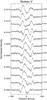 |
Fig. B.1 Stacked plot of the synthetic fits (dotted points) and the synthetic Stokes V profiles (grey solid lines) obtained from the dynamo model. |
 |
Fig. B2a Orthographic maps of the original dynamo simulation which serves as a synthetic model for the test inversion, The model is shown at four different rotational phases φ. |
 |
Fig. B2b Reconstructed surface field from 12 phase modulated Stokes V profiles. The number and order of the phases as well as the introduced noise correspond to the real observations of V410 Tau. Given the observational constraints imposed on this test inversion the dynamo model could be very well reproduced. |
In this section we want to examine if the inversion is able to retrieve a surface field topology as complicated as that of a simulated α2Ω-type dynamo with the given data set. The question that we want to investigate here goes beyond the testing of an inversion code with simplified surface topologies, what we want to do here is to seek a more direct answer to our problem, can we trust the hypothesis of our work that the reconstructed surface topology of V410 Tau is in fact similar to that of a given α2Ω-type dynamo simulation.
For that reason we synthesized from the α2Ω-dynamo simulation of Elstner & Korhonen (2005), 12 phase resolved spectra at phases which correspond to our observations. The dynamo model was scaled to have a peak field strength of 1920 G. The stellar parameter are those from V410 Tau given in Sect. 4.4. Noise is added according to the Bootstrap analysis in Sect. 3.2. The inversion with iMap is run with the same setup as the original inversion for V410 Tau, which also means that the inversion is stopped at the same noise level. Only Stokes V profiles are used for this magnetic inversion. The result is illustrated in the orthographic plots Figs. B2a and B2b as well as in the profile plot Fig. B.1. Given the number of available phases and the noise level in the data, the original magnetic field structure is remarkably good reproduced. Although the maximum field strength is not quite reached in the reconstruction shown in Fig. B2b one can see that the intertwined nature of the field structure and the rapid variation of the field lines around the polar region is well reproduced. The quality of the fit of the inversion relative to the original synthesized Stokes V profiles is shown in Fig. B.1. This demonstrates that with the given data set the inversion code can in fact reconstruct a surface field with a topology as complex as a α2Ω-type dynamo.
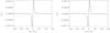 |
Fig. C1 Reconstructed SVD profile originating from all 929 spectral lines (left). The reconstruction is performed with all eigenprofiles. The “quasi-noise” level introduced by the line blends has a median absolute deviation (MAD) of 1.56 × 10⁻⁵. On the right, reconstructed SVD profile with only one eigenprofile corresponding to the largest eigenvalue. The difference between the reconstruction using the full set of eigenprofiles is hardly visible and the rms between them is 2.22 × 10⁻⁵. |
Appendix C: The influence of line blends
Here we want to investigate how much information about the line blends may get lost within the rank estimation of the truncated SVD procedure. Note that in our analysis we compare the SVD reconstructed line profile with the synthetic (weighted) mean of all contributing lines (929 lines for Stokes V and 56 for Stokes I) where all significant line blends are accounted for. One might suspect that if information about the line blends is leaked into the noise subspace it may lead to a mismatch between the synthesized line profiles and the reconstructed profile which may cause problems in the subsequent inversion.
Let us concentrate on the Stokes V profiles here and have a look on how line blends influence the resulting profile from the two-stage SVD reconstruction. Line blends affect the individual lines used in the observation matrix in different ways, they occur at different positions within the line profiles, and are of different strength and number. So it will be of interest to see how much of the blends are finally recognized as systematic and correlated effects within the SVD reconstruction. For that purpose we have modeled a simple monopole star with a homogeneous magnetic field of 10 G and a small rotational velocity of 5 km s-1. All other stellar parameters are assumed to be the same as that for V410 Tau. We synthesize the line profiles in the velocity domain and use a value of ± 150 km s-1, around the respective line center of each contributing line. For such a small rotational velocity the Stokes V signals are therefore much thinner than the used velocity range. This wide span of the velocity domain will give us additional information about the systematics introduced by the line blends relative to the base level (i.e. zero polarized continuum). The 929 lines are calculated without any noise. After calculating the line profiles and their respective line blends we applied the SVD analysis and used all available eigenprofiles for the reconstruction. The result of the two stage process is an average Stokes V profile that is the same as a regular average since we have used the entire set of eigenprofiles. In Fig. C1 on the left side we see the result of the SVD reconstruction. It is clearly seen that the Stokes V profile has its regular shape in spite of the many contributing line blends. The wiggling is the result of the line blends. Note again no noise is present in that synthetic test case. This wiggling of the base line (the continuum) shows no dramatic variation within the velocity range. We may quantify this wiggling in terms of a noise measure, and use the median absolute deviation (MAD) for that purpose which is defined as, MAD(V) = median(| V1 − median(V)|,...,|Vn − median(V)|), where median(V) is the median of the vector components of V. The MAD give us a value of 1.56 × 10⁻⁵. Given the strength of the reconstructed Stokes V signal, which has an amplitude comparable to that observed for V410 Tau, we can see that the blends introduce an effect that is below the noise level of the real reconstructed observations. How much information is lost if we would just use the eigenprofile corresponding to the largest eigenvalue? In that case we would pretend that our signal subspace is of dimension one and all significant signal information is comprised
within the first eigenprofile. Performing the two-stage SVD reconstruction under this assumption results in a Stokes V profile shown on the right side in Fig. C1. The difference between the reconstruction with the full set of eigenvectors and that using only a single eigenprofile is very small. We calculated the rms between the two reconstructed profiles which gives a value of 2.22 × 10⁻⁵. The contribution of the line blends relative to the Stokes signal for the set of 929 spectral lines used in this work is apparently very small, i.e. ten times smaller than the noise level deduced in Sect. 3.2. The remaining systematic effects introduced by the blending are essentially captured by the first eigenprofile which is also the signal carrying component. This demonstrates that the influence of line blends for the set of spectral lines used in this work is small and that the leakage of information carried by eigenprofiles belonging to smaller eigenvalues (i.e. noise space) is negligible.
Acknowledgments
The authors would like to thank Nadine Manset and the other CFHT staff for their support of the observations. K.G.S. is grateful to the German Science Foundation (DFG) for support under grant STR645/1. J.B.R. acknowledges support from the Natural Science and Engineering Research Council of Canada (NSERC).
References
- Bishop, C. M. 1995, Neural Networks for Pattern Recognition (Oxford University Press) [Google Scholar]
- Bouvier, J., & Bertout, C. 1989, A&A, 211, 99 [NASA ADS] [Google Scholar]
- Byrne, C. 2004, Inverse Problems, 103 [Google Scholar]
- Carroll, T. A., & Kopf, M. 2007, A&A, 468, 323 [NASA ADS] [CrossRef] [EDP Sciences] [Google Scholar]
- Carroll, T. A., Kopf, M., Ilyin, I., & Strassmeier, K. G. 2007, Astron. Nachr., 328, 1043 [NASA ADS] [CrossRef] [Google Scholar]
- Carroll, T. A., Kopf, M., & Strassmeier, K. G. 2008, A&A, 488, 781 [NASA ADS] [CrossRef] [EDP Sciences] [Google Scholar]
- Carroll, T. A., Kopf, M., Strassmeier, K. G., & Ilyin, I. 2009, in Cosmic Magnetic Fields: From Planets, to Stars and Galaxies (Cambridge Univ. Press), IAU Symp., 259, 633 [Google Scholar]
- Castelli, F., & Kurucz, R. L. 2004, IAU Symp., 210, poster A20 [Google Scholar]
- Donati, J.-F. 2001, Astrotomography, Indirect Imaging Methods in Observational Astronomy, eds. H. M. J. Boffin, D. Steeghs, & J. Cuypers, Lect. Notes Phys., 573, 207 [Google Scholar]
- Donati, J.-F. 2003, in Solar Polarization, eds. J. Trujillo-Bueno, & J. Sanchez Almeida, ASP Conf. Proc., 307, 41 [Google Scholar]
- Donati, J.-F., & Landstreet, J. D. 2009, ARA&A, 47, 333 [NASA ADS] [CrossRef] [MathSciNet] [Google Scholar]
- Donati, J.-F., Semel, M., Carter, B. D., Rees, D. E., & CollierCameron, A. 1997, MNRAS, 291, 658 [NASA ADS] [CrossRef] [MathSciNet] [Google Scholar]
- Donati, J.-F., Mengel, M., Carter, B. D., et al. 2000, MNRAS, 316, 699 [NASA ADS] [CrossRef] [Google Scholar]
- Donati, J.-F., Cameron, A. C., Semel, M., et al. 2003, MNRAS, 345, 1145 [NASA ADS] [CrossRef] [Google Scholar]
- Efron, B., & Tibshirani, R. J. 1994, An Introduction to the Bootstrap, eds. Taylor & Francis, Monographs on Statistics and applied Probability [Google Scholar]
- Egger, H., & Neubauer, A. 2005, Num. Math., 101, 643 [CrossRef] [Google Scholar]
- Elstner, D., & Korhonen, H. 2005, Astron. Nachr., 326, 278 [NASA ADS] [CrossRef] [Google Scholar]
- Engl, H. W., & Kugler P. 2004, Nonlinear inverse problems: theoretical aspects and some industrial applications, Optimization and Control of Complex Systems (Berlin: Springer) [Google Scholar]
- Engl, H. W., Hanke, & M. Neubauer, A. 1996, Regularization of Inverse problems, Mathematics and Its application, (Dordrecht, The Netherlands: Kluwer Academic Publishers) [Google Scholar]
- Gray, D. F. 2005, The observation and analysis of stellar photospheres, 3rd edn. (Cambridge University Press) [Google Scholar]
- Gregory, S. G., & Donati, J.-F. 2011, Astron. Nachr., 332, 1027 [NASA ADS] [CrossRef] [Google Scholar]
- Hanke, M. 1997, Inverse problems, 79 [Google Scholar]
- Hanke, M., Neubauer, A., & Scherzer, O. 1995, Num. Math., 72, 21 [Google Scholar]
- Hansen, P. C. 1990, SIAM J. Sci. and Stat. Comput., 11, 503 [CrossRef] [Google Scholar]
- Hatzes, A. P. 1995, ApJ, 451, 784 [NASA ADS] [CrossRef] [Google Scholar]
- Hussain, G. A. J. 2012, Astron. Nachr., 333, 4 [NASA ADS] [CrossRef] [Google Scholar]
- Jolliffe, I. T. 2002, Principal Components Analysys, Second Edition (New York: Springer) [Google Scholar]
- Joncour, I., Bertout, C., & Ménard, F. 1994, A&A, 285, L25 [NASA ADS] [Google Scholar]
- Johnstone I. M. 2001, On the distribution of the largest eigenvalue in principle component analysis, Ann. Statist., 2, 295 [Google Scholar]
- Kaltenbacher, B. Neubauer, A., & Scherzer, O. 2008, Iterative Regularization Methods for Nonlinear Ill-Posed Problems, Radon Series on Computational and applied Mathematics (Berlin: DeGruyter) [Google Scholar]
- Kitchatinov, L. L., Jardine, M., & Collier Cameron, A. 2001, A&A, 374, 250 [NASA ADS] [CrossRef] [EDP Sciences] [Google Scholar]
- Kochukhov, O., & Piskunov, N. 2002, A&A, 388, 868 [NASA ADS] [CrossRef] [EDP Sciences] [Google Scholar]
- Kochukhov, O., Makaganiuk, V., & Piskunov, N. 2010, A&A, 524, A5 [NASA ADS] [CrossRef] [EDP Sciences] [Google Scholar]
- Kupka, F., Piskunov, N., Ryabchikova, T. A., Stempels, H. C., & Weiss, W. W. 1999, A&AS, 138, 119 [NASA ADS] [CrossRef] [EDP Sciences] [MathSciNet] [PubMed] [Google Scholar]
- Küker, M., & Rüdiger, G. 1997, A&A, 328, 253 [NASA ADS] [Google Scholar]
- Küker, M., & Rüdiger, G. 1999, A&A, 346, 922 [NASA ADS] [Google Scholar]
- Martínez González, M. J., AsensioRamos, A., Carroll, T. A., et al. 2008, A&A, 486, 637 [NASA ADS] [CrossRef] [EDP Sciences] [Google Scholar]
- Moradi, H., Baldner, C., Birch, A. C., et al. 2010, Sol. Phys., 267, 1 [NASA ADS] [CrossRef] [Google Scholar]
- Paletou, F. 2012, A&A, 544, A4 [NASA ADS] [CrossRef] [EDP Sciences] [Google Scholar]
- Petit, P., Donati, J.-F., & Collier Cameron, A. 2002, MNRAS, 334, 374 [NASA ADS] [CrossRef] [MathSciNet] [Google Scholar]
- Piskunov, N., & Kochukhov, O. 2002, A&A, 381, 736 [NASA ADS] [CrossRef] [EDP Sciences] [Google Scholar]
- Piskunov, N. E., & Rice, J. B. 1993, PASP, 105, 1415 [NASA ADS] [CrossRef] [Google Scholar]
- Piskunov, N. E., Kupka, F., Ryabchikova, T. A., Weiss, W. W., & Jeffery, C. S. 1995, A&AS, 112, 525 [NASA ADS] [Google Scholar]
- Press, W. H., Flannery, B. P., Teukolsky, S. A., & Vetterling, W. T. 1992, Numerical Recipies (Cambridge University Press) [Google Scholar]
- Ramírez Vélez, J. C., Semel, M., Stift, M., et al. 2010, A&A, 512, A6 [NASA ADS] [CrossRef] [EDP Sciences] [Google Scholar]
- Reiners, A. 2006, A&A, 446, 267 [NASA ADS] [CrossRef] [EDP Sciences] [Google Scholar]
- Reiners, A., & Schmitt, J. H. M. M. 2003, A&A, 398, 647 [NASA ADS] [CrossRef] [EDP Sciences] [Google Scholar]
- Rempel, M. 2011, ApJ, 740, 15 [NASA ADS] [CrossRef] [Google Scholar]
- Rempel, M., Schüssler, M., & Knölker, M. 2009, ApJ, 691, 640 [NASA ADS] [CrossRef] [Google Scholar]
- Rice, J. B. 2002, Astron. Nachr., 323, 220 [NASA ADS] [CrossRef] [Google Scholar]
- Rice, J. B., & Strassmeier, K. G. 1996, A&A, 316, 164 [NASA ADS] [Google Scholar]
- Rice, J. B., & Strassmeier, K. G. 2000, A&AS, 147, 151 [NASA ADS] [CrossRef] [EDP Sciences] [Google Scholar]
- Rice, J. B., Strassmeier, K. G., & Kopf, M. 2011, ApJ, 728, 69 (Paper I) [NASA ADS] [CrossRef] [Google Scholar]
- Rüdiger, G., & Elstner, D. 1994, A&A, 281, 46 [NASA ADS] [Google Scholar]
- Rüdiger, G., & Hollerbach, R. 2004, The Magnetic Universe: Geophysical and Astrophysical Dynamo Theory (Wiley-VCH), 343 [Google Scholar]
- Rydgren, A. E., & Vrba, F. J. 1983, ApJ, 267, 191 [NASA ADS] [CrossRef] [Google Scholar]
- Savanov, I. S. 2012, Astron. Rep., 56/9, 722 [Google Scholar]
- Schrijver, C. J., & Title, A. M. 1999, Sol. Phys., 188, 331 [NASA ADS] [CrossRef] [Google Scholar]
- Schrijver, C. J., & Zwaan, C. 2000, Solar and stellar magnetic activity (New York: Cambridge University Press) [Google Scholar]
- Schrijver, C. J., De Rosa, M. L., Title, A. M., & Metcalf, T. R. 2005, ApJ, 628, 501 [NASA ADS] [CrossRef] [Google Scholar]
- Schüssler, M. 2005, Astron. Nachr., 326, 194 [NASA ADS] [CrossRef] [Google Scholar]
- Semel, M., Ramírez Vélez, J. C., Martínez González, M. J., et al. 2009, A&A, 504, 1003 [NASA ADS] [CrossRef] [EDP Sciences] [Google Scholar]
- Skelly, M. B., Donati, J.-F., Bouvier, J., et al. 2010, MNRAS, 403, 159 [NASA ADS] [CrossRef] [Google Scholar]
- Stelzer, B., & Neuhäuser, R. 2001, A&A, 377, 538 [NASA ADS] [CrossRef] [EDP Sciences] [Google Scholar]
- Stelzer, B., Fernández, M., Costa, V. M., et al. 2003, A&A, 411, 517 [NASA ADS] [CrossRef] [EDP Sciences] [Google Scholar]
- Stenflo, J. O. 1994, Solar magnetic fields: polarized radiation diagnostics, Astrophysics and Space Science Library (Dordrecht; Boston: Kluwer Academic Publishers) [Google Scholar]
- Strassmeier, K. G. 2009, A&ARv, 17, 251 [NASA ADS] [CrossRef] [Google Scholar]
- Strassmeier, K. G., & Rice, J. B. 1998, A&A, 330, 685 [NASA ADS] [Google Scholar]
- Strassmeier, K. G., Welty, A. D., & Rice, J. B. 1994, A&A, 285, L17 [NASA ADS] [Google Scholar]
- Vogt, S. S., Penrod, G. D., & Hatzes, A. P. 1987, ApJ, 321, 496 [NASA ADS] [CrossRef] [Google Scholar]
All Figures
|
Fig. 1 Stokes V eigenvalue spectrum of a V410-Tau observation (solid line) and the mean eigenvalue spectrum obtained from a bootstrap randomization process (dashed line) for the first 100 dimensions of rotation phase 0.014. The magnitude of the eigenvalues of the corresponding observation covariance matrix and the mean eigenvalues of all randomized matrices are plotted over the corresponding subspace dimension index. The crossing point at dimension 27 marks the dimension from which on the individual eigenprofiles contain no more significant information. |
| In the text | |
|
Fig. 2 Normalized Stokes I eigenvalue spectrum of the observation (solid line) and the noise variance (dashed line) for the first 20 subspace dimensions of rotation phase 0.014. For the purpose of a better illustration, the first three eigenvalues are not shown since they are significantly larger. The crossing point determines the signal subspace dimension to be 5. |
| In the text | |
|
Fig. 3 Reconstructed SVD Stokes V profiles for each rotational phase of V410 Tau. Each profile is reconstructed from an observation matrix with a sample size of 929 spectral lines. The averaged standard error is given together with the corresponding rotational phase. |
| In the text | |
|
Fig. 4 Reconstructed SVD Stokes I profiles for each rotational phase. For all reconstructed profiles an observation matrix with 56 spectral lines is used. The averaged standard error is given together with the corresponding rotational phase. |
| In the text | |
|
Fig. 5 Stacked plot of the synthetic fits (thick dashed lines) to the observed Stokes profiles (thin solid lines), on the left side Stokes I and on the right Stokes V. All spectral line profiles are normalized by the continuum intensity. |
| In the text | |
|
Fig. 6a Orthographic maps of the temperature distribution of V410 Tau at four different rotational phases φ. |
| In the text | |
|
Fig. 6b Orthographic maps of the magnetic field distribution of V410 Tau at four different rotational phases φ. The magnetic field is color coded and the field lines are proportional to the field strength (blue negative and red positive polarity). |
| In the text | |
|
Fig. 6c Orthographic maps of the temperature overplotted by the magnetic field lines at four different rotational phases φ. For a better visibility the positive fields are color coded in yellow while the negative fields are again in blue. As above the field lines are proportional to the strength of the field. |
| In the text | |
|
Fig. 7 Pseudo-Mercator projection of the three magnetic-field components; left radial, middle meridional, and right azimuthal. Note, that the lower x-axis is the longitudinal angle, while the upper x-axis gives the rotational phase. The dotted line indicates the limit for the visibility due to the stellar inclination. |
| In the text | |
|
Fig. 8 Intriguing structural similarity between the result of our magnetic surface reconstruction (left) and an α2Ω-dynamo simulation which is scaled to a surface field strength of 1.9 kG (right). |
| In the text | |
|
Fig. A1a Temperature error map in orthographic projection at four different rotational phases. The maximum rms value is 80 K and the mean rms value is 50 K. Regions below a latitude of –30° are set to a constant value and do not participate in the error estimation. |
| In the text | |
|
Fig. A1b Radial magnetic field error map in orthographic projection at four rotational phases, the maximum rms value is 125 G and the mean rms value is 64 G. |
| In the text | |
|
Fig. A1c Meridional magnetic field error in orthographic projection, the maximum rms value here is 101 G and the mean rms value is 51 G. |
| In the text | |
|
Fig. A1d Azimuthal magnetic field error in orthographic projection with a maximum rms value of 106 G and a mean value of 52 G. |
| In the text | |
|
Fig. B.1 Stacked plot of the synthetic fits (dotted points) and the synthetic Stokes V profiles (grey solid lines) obtained from the dynamo model. |
| In the text | |
|
Fig. B2a Orthographic maps of the original dynamo simulation which serves as a synthetic model for the test inversion, The model is shown at four different rotational phases φ. |
| In the text | |
|
Fig. B2b Reconstructed surface field from 12 phase modulated Stokes V profiles. The number and order of the phases as well as the introduced noise correspond to the real observations of V410 Tau. Given the observational constraints imposed on this test inversion the dynamo model could be very well reproduced. |
| In the text | |
|
Fig. C1 Reconstructed SVD profile originating from all 929 spectral lines (left). The reconstruction is performed with all eigenprofiles. The “quasi-noise” level introduced by the line blends has a median absolute deviation (MAD) of 1.56 × 10⁻⁵. On the right, reconstructed SVD profile with only one eigenprofile corresponding to the largest eigenvalue. The difference between the reconstruction using the full set of eigenprofiles is hardly visible and the rms between them is 2.22 × 10⁻⁵. |
| In the text | |
Current usage metrics show cumulative count of Article Views (full-text article views including HTML views, PDF and ePub downloads, according to the available data) and Abstracts Views on Vision4Press platform.
Data correspond to usage on the plateform after 2015. The current usage metrics is available 48-96 hours after online publication and is updated daily on week days.
Initial download of the metrics may take a while.