| Issue |
A&A
Volume 548, December 2012
|
|
|---|---|---|
| Article Number | A56 | |
| Number of page(s) | 14 | |
| Section | Stellar structure and evolution | |
| DOI | https://doi.org/10.1051/0004-6361/201219832 | |
| Published online | 21 November 2012 | |
X-shooter spectroscopy of young stellar objects
I. Mass accretion rates of low-mass T Tauri stars in σ Orionis⋆
1 INAF/Osservatorio Astrofisico of Arcetri, Largo E. Fermi, 5, 50125 Firenze, Italy
e-mail: This email address is being protected from spambots. You need JavaScript enabled to view it.
2 Department of Planetary Science, Lunar and Planetary Lab, University of Arizona, 1629, E. University Blvd, 85719 Tucson AZ, USA
3 INAF/Osservatorio Astronomico di Capodimonte, Salita Moiariello, 16, 80131 Napoli, Italy
4 INAF/Osservatorio Astronomico di Palermo, Piazza del Parlamento 1, 90134 Palermo, Italy
5 DIAS/Dublin Institute for Advanced Studies, Burlington Road, Dublin 4, Ireland
6 ESO/European Southern Observatory, Karl-Schwarzschild-Strasse 2, 85748 Garching bei München, Germany
Received: 17 June 2012
Accepted: 27 September 2012
Abstract
We present high-quality, medium-resolution X-shooter/VLT spectra in the range 300−2500 nm for a sample of 12 very low mass stars in the σ Orionis cluster. The sample includes eight stars with evidence of disks from Spitzer and four without disks, with masses ranging from 0.08 to 0.3 M⊙. The aim of this first paper is to investigate the reliability of the many accretion tracers currently used to measure the mass accretion rate in low-mass young stars and the accuracy of the correlations between these secondary tracers (mainly accretion line luminosities) found in the literature. We use our spectra to measure the accretion luminosity from the continuum excess emission in the UV and visual; the derived mass accretion rates range from 10-9 M⊙ yr-1 down to 5 × 10-11 M⊙ yr-1, allowing us to investigate the behavior of the accretion-driven emission lines in very low mass accretion rate regimes. We compute the luminosity of ten accretion-driven emission lines from the UV to the near-IR, which are all obtained simultaneously. In general, most of the secondary tracers correlate well with the accretion luminosity derived from the continuum excess emission. We recompute the relationships between the accretion luminosities and the line luminosities, and we confirm the validity of the correlations given in the literature, with the possible exception of Hα. Metallic lines, such as the CaII IR triplet or the Na I line at 589.3 nm, show a larger dispersion. When looking at individual objects, we find that the hydrogen recombination lines, from the UV to the near-IR, give good and consistent measurements of Lacc that often better agree than the uncertainties introduced by the adopted correlations. The average Lacc derived from several hydrogen lines, measured simultaneously, have a much reduced error. This suggests that some of the spread in the literature correlations may be due to the use of nonsimultaneous observations of lines and continuum. Three stars in our sample deviate from this behavior, and we discuss them individually.
Key words: stars: low-mass / accretion, accretion disks / line: formation / open clusters and associations: individual:σOrionis
Based on observations collected at the European Southern Observatory, Chile. Program 084.C-0269(A), 086.C-0173(A).
© ESO, 2012
1. Introduction
Accretion of matter onto T Tauri stars is an important aspect of the star formation process and plays a fundamental role in shaping the structure and evolution of proto-planetary disks. Magnetospheric accretion (Uchida & Shibata 1985; Köenigl 1991; Shu et al. 1994) is the accepted paradigm that explains the accretion in classical T Tauri stars (CTTSs) and lower-mass objects. In this family of models, material from the inner edge of the disk is channelled through the stellar magnetosphere field lines and flows onto the star.
In a CTTS it is possible to identify two different regions in the magnetospheric accretion model structure: the accretion columns and the hot spots on the stellar surface. In the accretion columns there is gas that is accreting onto the star channelled along the magnetic field lines, while the hot spots are produced where the infalling material impacts onto the stellar surface. The accretion luminosity is released as continuum and line emission, formed in the hot spots and/or in the accreting gas columns.
The intensity of the continuum emission, its wavelength dependence, and the intensity and profiles of the various emission lines can be used to derive quantitative information about the accretion process itself (e.g., Hartmann et al. 2006). In particular, the integrated continuum and line luminosity Lacc is proportional to the mass accretion rate, which can be computed from it once the ratio of the stellar mass to radius is known. Measurements of Lacc require well-calibrated observations of the continuum flux over a wide range of wavelengths, as well as an adequate knowledge of the photospheric and chromospheric spectrum of the star, which need to be subtracted from the observed flux to isolate the accretion emission. This has been possible for a relatively small sample of objects only (Hartigan et al. 1995, 1991; Muzerolle et al. 2003; Valenti et al. 1993; Calvet & Gullbring 1998; Gullbring et al. 1998; Herczeg & Hillenbrand 2008, hereafter HH08). However, it has been noticed that in these objects the luminosity or flux of several lines correlates quite well with Lacc. Using these correlations, it has been possible to estimate Lacc and therefore Ṁacc in many young stars. These secondary indicators span a huge range of wavelength. In the far-ultraviolet (FUV) Herczeg et al. (2002) and Yang et al. (2012) found that the OIλ103.4 nm triplet, SiIVλ139.4, 140.3 nm doublet and CIVλ154.9 nm doublet are tightly correlated with Lacc. In the soft X-rays, Telleschi et al. (2007) and Curran et al. (2011) found that the low-density plasma component in the post-shock region correlates with Ṁacc. From the near-UV to the near-IR several hydrogen recombination lines can be used to estimate Lacc (Hα, Hβ, H11, Paβ, Paγ), as well as other lines CaIIλ854.2 nm, CaIIλ866.2 nm, HeIλ587.6 nm, NaIλ589.3 nm, as shown by Fang et al. (2009), Mohanty et al. (2005), HH08, Natta et al. (2004), and Gatti et al. (2008), among many others. The excess emission in the U-band is also well correlated with Lacc (Gullbring et al. 1998), and can be used to measure it when the reddening is low. Finally a widely used accretion indicator is the Hα 10% line width, which has been found to be correlated with Ṁacc (Natta et al. 2004), although with high dispersion. The existence of secondary indicators in different regions of the spectrum is very important, as the more direct method of measuring Lacc integrating the excess emission over the whole wavelength range is often impractical or altogether impossible. It is, therefore, necessary to estimate the relative reliability of the different indicators over the widest possible range of the parameters, i.e., Lacc, Ṁacc, or M∗.
When several indicators are measured for the same object, the accretion rate may differ by a factor of ten or more. Since in many cases different indicators are not observed simultaneously, one possible reason is the well-known time variability of the pre-main sequence stars (Joy 1945; Herbst et al. 1994, 2007). Up to now it has been difficult to observe several accretion tracers simultaneously, especially because they span from the UV wavelength region (e.g., the Balmer series lines) to the near-IR (e.g., Paβ, Paγ and Brγ hydrogen recombination lines). This means that when comparing nonsimultaneous observations of these indicators an error caused by the time variability cannot be ruled out. This observational gap can be filled in with the use of broad spectral range spectrographs such as X-shooter at the VLT. X-shooter is an ideal instrument for comparing different accretion tracers because it simultaneously covers the wavelength range from ~300 to ~2500 nm.
We present here a systematic simultaneous study of primary and secondary accretion indicators in young stellar objects. Our target sample is composed of young low mass T Tauri stars in the σ Orionis star-forming region. σ Orionis is located at a distance of ~360 pc (Hipparcos distance 352 pc, Brown et al. 1994, Perryman et al. 1997) and has an age of ~3 Myr (Zapatero-Osorio et al. 2002; Fedele et al. 2010). The region has negligible extinction (Béjar et al. 1999; Oliveira et al. 2004), and has been extensively studied in the optical, X-rays, and infrared (e.g. Rigliaco et al. 2011a; Kenyon et al. 2005; Zapatero-Osorio et al. 2002; Jeffries et al. 2006; Franciosini et al. 2006; Hernandez et al. 2007).
The observations presented in this paper have been carried out as part of a larger study of the accretion properties in very low mass stars and brown dwarfs in nearby star-forming regions with X-shooter (Alcalà et al. 2011; Alcalà et al., in prep.).
In this paper, we present results related to the accretion phenomena. Additional results about the properties of the nonaccreting objects and wind phenomena will be shown in upcoming papers of Manara et al. (in prep.) and Rigliaco et al. (in prep.), respectively.
The structure of the paper is as follows. Section 2 summarizes the details of the observations, data reduction, and the instrument set-up. Section 3 describes the properties of the sample. In Sect. 4 we discuss how the accretion luminosities and mass accretion rates are measured from the excess continuum emission. The measurement of Lacc from the emission lines is described in Sect. 5. In Sects. 5.1 and 5.2 we compare all indicators that were observed simultaneously with X-shooter, and investigate their reliability as accretion tracers. Notes on individual targets are given in Sect. 5.3. A summary can be found in Sect. 6.
2. Observations and data reduction
Journal of the observations.
The sample analyzed in this paper has been observed with X-shooter on VLT as part of the Italian INAF/GTO program on star-forming regions (Alcalà et al. 2011). Observations were performed in visitor mode on 21, 23 and 24 December 2009 and 11−12 January 2011. We observed 12 objects, obtaining medium-resolution spectra covering ~300−2500 nm range. The observations log (Table 1) lists the coordinates of the targets, the exposure time, and the abbreviated object names used throughout this paper (the last row of this table reports information of a class III star with spectral type M4, observed within the GTO program in the Lupus star-forming region. This star has been used as class III template in this paper).
The targets were observed in nodding mode with the 11′′ × 1.0′′ slit in the ultaviolet arm (UVB-arm), and with 11′′ × 0.9′′ slit in the visual (VIS) and near-infrared (NIR) arms. This instrument configuration yields a resolution R ~ 5100 over the UVB-arm, which covers a wavelength range 300−590 nm, and the NIR-arm, which covers a wavelength range 1000 − 2480 nm, while with the VIS-arm (wavelength range from ~580 nm to ~1000 nm) we achieved a resolution R ~ 8800.
The data reduction was performed independently for each spectrograph arm using the X-shooter pipeline version 1.1.0, following the standard steps, which include bias subtraction, flat-fielding, optimal extraction, wavelength calibration, and sky subtraction. The extraction of the 1D spectra and the subsequent data analysis was performed in STARE mode for UVB and VIS-arms, and in NODDING mode for the NIR-arm. Flux calibration has been achieved using the context LONG within MIDAS1. For this purpose, a response function was derived by interpolating the counts/standard-flux ratio of the flux standards (observed the same night as the objects, generally under photometric sky conditions), with a third-order spline function, after airmass correction. The flux-match of the three arms is excellent (Alcalà et al. 2011), and the flux-calibrated spectra show on average a very good agreement with the flux derived from photometric measurements available in the literature. Only in a few cases observed in not completely photometric conditions, we have adjusted the flux-calibrated spectra shifting the spectra on the photometric flux. The data were analyzed using the task SPLOT within the IRAF2 package.
3. The sample
The 12 targets for this study have been selected among the sample observed in the U-band by Rigliaco et al. (2011a) with FORS1 at the VLT, covering a range of masses between ~0.08 − ~0.3 M⊙. Objects with mid-infrared colors that suggest they are young stars possessing disks (class II), and sources without obvious IR excess emission (class III) to be used as template were selected.
Spectral types (SpT) were estimated using the various indices by Riddick et al. (2007). These authors provide calibrations specifically for young M dwarfs. The flux ratios were derived from the flux-calibrated optical spectra. The final SpT assigned to a given object was estimated as the average SpT resulting from the various indices. The effective temperature Teff was obtained for each star using the temperature scale of Luhman et al. (2003). Luminosities were then computed using the I-band magnitudes (as listed in Table 2), and the bolometric correction for zero age main sequence (ZAMS) stars as reported by Luhman et al. (2003). As described in Sect. 1, the distance of σ Ori is 360 pc and the extinction is negligible. The uncertainty in the SpT of about half a subclass corresponds to a typical error of ± 70 K on the photospheric effective temperature. The error on the luminosity is caused by the adopted bolometric correction (which is linked to the error on Teff), to the uncertainty on the measurement of the I-band magnitude (assumed to be ~0.2 mag), and to the uncertainty on the distance of the cluster, which may vary from ~330 pc (Caballero 2008) to ~470 pc (De Zeeuw et al. 1999). A detailed analysis of the error caused by the uncertainty on the distance was given by Rigliaco et al. (2011c). We estimate a typical uncertainty in luminosity of ~0.2 dex. Based on the location of the targets on the HR diagram and on a comparison with the Baraffe et al. (1998) evolutionary tracks, we have estimated the object masses and ages. The properties of the stars in our sample are summarized in Table 2. The determinations of the radius and of the mass are also affected by the distance uncertainty. We assume a typical error on these parameters of ~0.05 dex.
Stellar parameters and observed properties.
As expected from previous photometric classification (Hernandez et al. 2007), eight stars in our sample show a spectral energy distribution (SED, in Fig. 1) with IR excess emission, in particular in the IRAC spectral range (from 3.6 μm to 8.0 μm), indicating the presence of an optically thick circumstellar disk, i.e., they are class II objects (see Fig. 1a). The remaining four stars in our sample show the typical color of the stellar photospheres and no IR excess. The SEDs of these class III objects are shown in Fig. 1b. The SEDs shown in Fig. 1 are scaled to the J-band flux, while in the following figures the spectra are normalized to 700 nm. Previous work on the veiling (Hartigan et al. 1995; White & Ghez 2001; Fischer et al. 2011) show that there may be some excess continuum at and beyond this wavelength, but in our sample the veiling is low (see the following sections), allowing us to use the region around 700 nm to normalize the spectra. In Fig. 1, the black points are the available photometry, U-band from Rigliaco et al. (2011a), BVRI from the literature (see Rigliaco et al. 2011a), JHK from 2MASS photometry (Cutri et al. 2003), z,Y from the UKIDSS survey, and IRAC/MIPS magnitudes from the Spitzer survey. In Fig. 1a, the red curves represent the photospheric contribution obtained using the NextGen models (Hauschildt et al. 1999a,b; Allard et al. 2000), normalized to the J-band, and for comparison purpose, we show as a gray region, the median SED for CTTSs in Taurus derived from previous ground-based and IRAS data (D’Alessio et al. 1999).
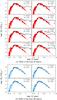 |
Fig. 1 SEDs for the sample analyzed in this paper. Effective temperature of the adopted photospheric template is indicated as well as the name of the target. For all stars with excess above the photosphere, the median disk SED in Taurus (gray region) is displayed, scaled to the J-band flux. Black points are the photometric data (we did not apply any correction for the extinction because the reddening in the σOri star-forming region is negligible (Béjar et al. 1999; Oliveira et al. 2004)). |
4. Balmer and Paschen continua as accretion diagnostics
The accretion luminosity is released as continuum and line emission over a wide range of wavelengths. In general, the continuum luminosity dominates over the emission in lines, which is generally neglected in the literature, although, as we will see in Sect. 4, this may not be the case at a low mass-accretion rate. We will define in the following Lacc,c to be the continuum luminosity only.
The excess emission is clearly seen in the Balmer continuum, where the photospheric and chromospheric emission of the stars is very low. Of the eight class II stars in our sample, six show clear evidence of it, as seen in Fig. 2, where the spectrum of each star is compared to that of a class III object of similar spectral type, normalized at 700 nm (the adopted class III template stars for each class II object are listed in Table 3).
Most stars clearly show the Balmer jump at the Balmer edge (note that the Balmer limit occurs at λ346.7 nm, but the line blending in the Balmer series shifts the apparent jump to 370 nm).
In Table 3 we list the values of the observed Balmer jump (BJobs), defined as the ratio of the flux at 360 nm to the flux at 420 nm, and of the intrinsic Balmer jump (BJintr), measured after subtracting off the photospheric template from the class II star. This value is generally computed after dereddening the spectra, but in the σ Orionis star-forming region the extinction is negligible (Oliveira et al. 2004). The observed Balmer jump ranges between ~0.2 and ~3.5 for the class II objects, as shown in Table 3, Col. 3. BJobs for the class III objects spans between ~0.2 and ~0.5. In two class II objects, namely SO587 and SO1266, BJobs is in the same range as that of the class III stars. These objects will be discussed below. The intrinsic Balmer jump ranges between ~1.4 and ~14.4, as reported in Table 3, Col. 4.
The accretion continuum emission in the Paschen continuum (i.e., for 346 nm ≲ λ ≲ 820 nm) is usually a smaller fraction of the photospheric continuum than in the UV and it is more easily detected as veiling3 of the photospheric absorption lines, which are filled-in by the excess continuum.
Figure 3 shows the CaI λ422.6 nm line for the eight class II stars in our sample. We find very little evidence (if any) of veiling in 6 out of 8 objects. Only in two cases (SO397 and SO1260) the CaI line is clearly filled-in. In some of our stars (SO490 and SO500), the CaI 422.6 nm line is slightly shallower than expected from a comparison to the nonaccreting template. However, this is likely due to the overlapping emission of many lines. Moreover, the depth of this line may also be affected by stellar rotation (Mauas & Falchi 1996; Short et al. 1997).
To compute Lacc,c, we modeled the excess luminosity as the emission of a slab of hydrogen of fixed electron density (Ne), temperature (Te), and length (L), under the assumption of local thermal equilibrium (LTE). Similar models, although very simple and not realistic, have been used by Valenti et al. (1993) and HH08, among others, and have been found to reproduce the wavelength dependence of the observed excess emission well. These models allow us to account for the ultraviolet emission outside of the observed range and to interpolate between the wavelength of the veiled lines. We added the emission of the slab to that of the adopted class III template, varying the model parameters until we found a satisfactory fit to the observed continuum over the whole spectral range from UV to red. There are five free parameters, the slab parameters (Te,Ne,L), a scale factor for the slab emission, and the normalization constant of the class III template, which all need to be constrained simultaneously. We have varied the slab parameters over a wide range of values, and adopted different class III templates whenever possible.
The best-fit models are shown in Fig. 2 for the UV continuum and Fig. 3 for the CaI line at 422.6 nm. Figure 4 shows the normalization region around 700 nm. In 7 out of 8 objects the excess emission is negligible; only in the object SO1260 this is not the case and the template normalization needs to take this into account.
The accretion luminosity is given by the emission of the adopted slab model scaled to fit the data as described above. In 6 out of 8 objects the excess luminosity is clearly detected; in two cases (SO587 and SO1266) we can only determine upper limits. It is interesting to note that the Balmer continuum accounts for about 50% of Lacc,c in all objects but the two strongest accretors (SO397, where it drops to 17%, and SO1260, 26%). In these two objects the excess emission is dominated by the Paschen continuum. The correction for the emission shortward of 330 nm, which is the shortest observed wavelength in most of our spectra, is typically a factor of two.
The uncertainty on Lacc,c derives firstly from the noise of the target and the template spectra, then from degeneracies in the slab model that affect the correction for the emission below 330 nm, the difficulty of constraining the emission in the Paschen continuum in objects where line veiling is not detected, and the choice of the class III template. The large set of models we computed suggests that the first is never higher than 20 − 30% and the uncertainty introduced by the definition on the Paschen continuum is on the same order. The slab parameters themselves are poorly constrained as many trade-offs are possible, all resulting, however, in very similar emission spectra. As far as the choice of the class III is concerned, we found that, when two templates provide an equally good fit to the observed spectra, the corresponding values of Lacc,c are within 10% of each other. In one case (SO848), we found that none of our class III templates with similar spectral type reproduces the observations very well. However, even in this case, the two values of Lacc,c (obtained using Sz94 and SO797 as templates) differ by only 16%. In summary, a total uncertainty of 50% is adopted for accretion luminosities Lacc,c calculated with this method, which incorporates uncertainties in distance, bolometric corrections, and the exclusion of emission lines estimated in the next subsection.
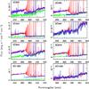 |
Fig. 2 Comparison between the observed spectra and the fit obtained considering the slab model. Red spectra represent the observed emission in the region of the Balmer jump after a smoothing by boxcar seven. The green spectra show the photospheric template, the cyan lines are the synthetic accretion spectra from the slab model. The sum of the slab model plus the template is shown by the blue spectra. |
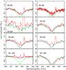 |
Fig. 3 Ca I λ422.6 nm absorption line in the X-shooter spectra (red-solid lines). The green line shows the spectrum of the adopted class III template and the blue-dashed line the adopted model with the emission predicted from the slab model added to the template. Fe I emission lines at 421.6, 422.7 and 423.3 nm can also be identified. |
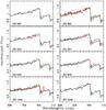 |
Fig. 4 Region around 700 nm. The red-solid lines shows the class II spectra, the green line shows the spectrum of the adopted class III template and the blue-dashed line the adopted model with the emission added to the template. |
Line contribution to L acc
Our estimate of Lacc,c is obtained from the continuum emission of the accretion slab model without taking into account the contribution of the emission lines (which may vary with mass accretion rates and stellar parameters). Although the energy budget in the lines can be large, this is common practice, and excluding the line contribution makes our accretion luminosity estimates comparable to those of previous works (HH08, Valenti et al. 1993; Calvet & Gullbring 1998).
To assess the importance of line emission we computed their contribution to the accretion luminosity. The fraction of luminosity in the Balmer lines with respect to the continuum accretion luminosity Lacc,c is reported in Table 3, Col. 5. We estimate that the high-n Balmer lines (from the 12th hydrogen recombination line (λ = 375.0 nm) to the pseudo-continuum) contain a fraction between ~0.1 and ~0.4 of the continuum accretion luminosity in 5 out of 8 of the class II objects. In SO500 the luminosity in the hydrogen recombination lines is similar to the continuum accretion luminosity, and in SO587 and SO1266, where there is an upper limit in the continuum accretion luminosity, the fraction of luminosity in the hydrogen lines is higher than one. This is not surprising because these lines are likely caused by the chromospheric activity in these two stars, and not by the accretion luminosity (see Sect. 5.3).
Accretion luminosities and mass accretion rates.
5. Emission lines as accretion diagnostics
As described in Sect. 1, magnetospheric accretion produces emission lines that span from UV to IR wavelengths; these lines can be used to obtain an estimate of the accretion luminosity, and are also signatures of the chromospheric activity of the star.
The Hα line luminosity has been found to be strictly related to the accretion luminosity (e.g., Muzerolle et al. 2003, 2005, HH08; Dahm 2008; Fang et al. 2009). This kind of relation has been found for other hydrogen recombination lines as well (Hβ, Hγ, H11, Paβ and Paγ; e.g. Muzerolle et al. 1998, 2003; Natta et al. 2004, HH08; Dahm et al. 2008). Unfortunately, the low signal-to-noise ratio of our NIR spectra at λ > 2100 nm prevents us from detecting the Brγ line reliably, hence we do not provide measurements for this line.
The CaII near-IR triplet (λλ849.8, 854.2, 866.2 nm) broad emission components are commonly attributed to accretion shocks very close to the stellar surface (Batalha et al. 1996). In particular, this triplet has been used to detect accretion in low- and intermediate-mass stars (Hillenbrand et al. 1998; Muzerolle et al. 1998; Rhode et al. 2001; Mohanty et al. 2005).
The HeI emission line at 587.6 nm is another feature that has been used to characterize accretion processes. Among pre-main-sequence stars, broadened emission line profiles of HeI transition have been linked with magnetospheric accretion flows, as demonstrated by Muzerolle et al. (1998).
Another line that moderately correlates with the accretion luminosity is the NaIλ589.3 nm line which is supposed to be produced in the magnetospheric infall zone. The HeI and NaI lines are usually associated with both infall and outflows (Hartigan et al. 1995; Beristain et al. 2001; Edwards et al. 2006) but throughout this paper they are used as tracers of the accretion.
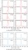 |
Fig. 5 Hα line profiles normalized at 700 nm (class II red lines, panel a), and class III cyan lines, panel b)). The class II line profiles exhibit diverse morphologies that presumably arise from differing accretion rate values, gas temperature, and geometries (inclinations and magnetospheric radii). |
The width of the Hα line at 10% of the peak has been extensively used to discriminate between accreting and not-accreting objects and to derive an estimate of the mass accretion rate (Natta et al. 2004; White & Basri 2003). Indeed, as we can clearly see from Fig. 5, many of the class II objects have a broader Hα line profile than the class III targets. However, in this work we decided not to use the Hα 10% line width to measure accretion rates, because, as pointed out by Natta et al. (2004), it does not provide accurate measurements of Ṁacc for individual objects.
Tables 4 and 5 list fluxes and equivalent widths (EWs) for the lines described above. We measured emission line fluxes and equivalent widths by fitting Gaussian profiles to the observed lines with the SPLOT/IRAF task. Where the line does not have a Gaussian-like profile, the line flux and EW are measured by directly integrating the flux along a window that includes the entire line (Fig. 5 presents a compilation of the Hα line profiles for our class II and class III sources). The errors on the EWs and fluxes were computed using a Monte Carlo approach: we added a normally distributed noise to the spectrum, following the error at each wavelength, and gave as error the standard deviation of the EW distribution of 1000 such spectra (Pascucci et al. 2011). The errors on the flux determination are larger for the fainter lines, as the continuum calibration around these lines is more uncertain. Typically we estimate errors between 1 − 5% for fluxes higher than 1.0 × 10⁻¹⁶ erg/cm2/s, and of ~10% for fainter fluxes.
Emission lines fluxes and equivalent widths of the Hα, Hβ, Hγ, H11, and HeI lines were measured for all class II objects in our sample. NaI, CaII λ854.2, and CaII λ866.2 were measured for all our targets except for one, two, and three objects, respectively, while we do not have an estimate of the Paγ, and Paβ for SO1266 because we completely missed the portion of the spectrum related to the NIR arm because of problems during the observations.
Hydrogen recombination line equivalent widths and fluxes.
Fluxes and equivalent widths of other lines used as accretion indicators.
Knowing the emission line fluxes Fline from the flux-calibrated spectrum, the line luminosities are given by  (1)where D is again the adopted distance of 360 pc. To determine accretion luminosities using the measured line fluxes, we used empirical relationships between the observed line luminosities and the accretion luminosity or mass accretion rates (HH08, Mohanty et al. 2005; Fang et al. 2009; Natta et al. 2004; Gullbring et al. 1998). These relationships were calibrated on relatively small samples of well-studied T Tauri stars and brown dwarfs, for which the accretion luminosity was derived by fitting the observed optical veiling with magnetospheric accretion models (Gullbring et al. 1998, for low-mass stars in the mass range between ~0.25−0.9 M⊙, and Calvet et al. 2004, for intermediate-mass T Tauri stars in the mass range between 1.5 − 4 M⊙), or, for brown dwarfs, the Hα line profile (Muzerolle et al. 2003).
According to these studies, the accretion luminosity can be computed from the line luminosity as  (2)where the coefficients a and b are summarized in Table 6 together with their origin in the literature. In the case of the CaII lines the equivalent widths were converted into line flux per stellar surface area, and then correlated directly with Ṁacc:
  (3)
(3)
Table 7 reports the calculated accretion luminosity for each star based on the different emission lines. To distinguish these values from those obtained from the continuum slab model, we denote the line-based accretion luminosities with Lacc,l throughout the remainder of the paper. Table 7 lists also the weighted mean accretion luminosity obtained from the secondary indicators, ⟨ Lacc,l ⟩ .
The accretion luminosity can be converted into mass accretion rate, Ṁacc according to  (4)
(4)
Line luminosity vs. accretion luminosity relationships for selected accretion indicators.
where G is the universal gravitational constant and the factor  ~ 1.25 is estimated by assuming that the accreting gas falls onto the star from the truncation radius of the disk (Rin ~ 5 R∗; Gullbring et al. 1998). The error introduced by this assumption on the measured mass accretion rates, considering that Rin for a pre-main sequence star can span from 3 to 8 R∗, is less than 20%. The stellar masses and radii are listed in Table 2. Note that the values of Lacc for the two CaII IR lines are derived from the mass accretion rate, computed from Eq. (3), and the standard relation between Lacc and Ṁacc (Eq. (4)).
5.1. Comparison of the accretion indicators
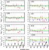 |
Fig. 6 Comparison between all accretion indicators listed in Table 6. The red dots are our estimates of the accretion luminosity, the red arrows are the upper limits, the yellow triangles refer to Lacc obtained from the U-band excess emission, which was observed non-simultaneously with the other indicators. The green dashed line is the average Lacc,l computed considering all secondary indicators; the green shaded region is the 1σ uncertainty in the average Lacc,l. The blue line is Lacc,c obtained using the excess continuum emission (dashed blue line for the upper limits). |
Figure 6 displays the Lacc,l values of Table 7 (red circles) and also the accretion luminosity derived by Rigliaco et al. (2011a − c) using the nonsimultaneous U-band excess emission (yellow triangle). Even though all accretion indicators except for the U-band were observed simultaneously, for a given star the spread between different values of Lacc,l is quite large, typically about one order of magnitude. However, as we have shown for the brown dwarf SO500 in Rigliaco et al. (2011b), for most of the stars analyzed here all values are consistent within the large error bars, and the average Lacc,l has a smaller uncertainty (green line in Fig. 6). In particular, the total errors on Lacc,l for each indicator are caused by the error on the line fluxes, on the adopted distance, and on the relationship used to estimate Lacc,l. The uncertainties on the flux and distance (which are about a factor 1.5 on the total accretion luminosity) are negligible with respect to the error caused by the assumed relationship, which corresponds to an uncertainty on Lacc,l of about a factor three. The uncertainty on ⟨ Lacc,l ⟩ (which by our definition excludes the estimate from the U-band excess emission) computed averaging the accretion luminosity for each indicator weighted by the corresponding error and neglecting the upper limits, is about a factor two.
In five stars of the sample discussed in this paper, SO397, SO490, SO500, SO646, and SO1260, the accretion luminosity obtained from the Balmer excess continuum (blue line) is within the 1σ uncertainty of the average accretion luminosity obtained by using the secondary accretion indicators. The three cases for which we found no good agreement will be discussed in Sect. 5.3.
In Fig. 7 we show for each star the average mass accretion rate derived from Lacc,l with Eq. (4) (Ṁacc,l) versus the mass accretion rate obtained with the same formula from the continuum accretion luminosity (Ṁacc,c). From this small sample we can conclude that the two quantities agree within the 1σ error (except for the cases discussed in Sect. 5.3) and do not show any robust trend with increasing Ṁacc,l. However, the sample considered here is small, and this question could be explored in more detail on a bigger sample of objects.
5.2. Reliability of the accretion tracers
One way to investigate the reliability of the accretion tracers, and the relation between accretion continuum luminosity (Lacc,c) and the accretion luminosity from the secondary indicators (Lacc,l), is comparing Lacc,c with the secondary tracers line luminosities or fluxes, including the sample analyzed here with those available in the literature. We recomputed the relationships between Lacc,l and Lacc,c after adding our new X-shooter data for σ Ori to the historical samples of accreting TTS published previously. These results are given in Table 8 and are discussed in the following subsections.
Estimated log Lacc (L⊙) from the secondary accretion indicators.
5.2.1. Hα, Hβ, and HeI
For the Hα, Hβ, and HeI lines as accretion tracers, we refer to Fang et al. (2009). They collected young stellar objects with measured Hα, Hβ and HeI emission line luminosities from the literature (Gullbring et al. 1998, HH08; and Dahm et al. 2008 for Hα; Gullbring et al. 1998 and HH08 for Hβ, and HH08; and Dahm et al. 2008 for HeI) for a sample of low-mass stars and brown dwarfs in the Taurus Molecular Cloud and the young open cluster IC 348. Figure 8 shows the comparison between the relationships found by Fang et al. (2009) (gray short-dashed line and gray crosses), by HH08 (black long-dashed line and black asterisks), and by us (green solid line and red dots). The correlations found by HH08 and by Fang et al. (2009) have been computed by least-square fitting the point distributions and neglecting the upper limits. We did the same adding to the Fang et al. (2009) sample the targets analyzed in this paper.
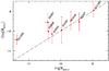 |
Fig. 7 Comparison between the mass accretion rates computed from the average of all indicators (Ṁacc,l) and Ṁacc,c. |
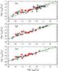 |
Fig. 8 Relationship between selected line luminosities and the accretion continuum luminosity. The red dots and arrows are the sample analyzed in this paper, the black asterisks and arrows refer to the sample analyzed by HH08. The gray crosses are the sample collected by Fang et al. (2009). The gray short-dashed line corresponds to the relation found by Fang et al. (2009). The black long-dashed line is the relation found by HH08, computed ignoring the upper limits in Lacc. The green lines correspond to the relations found using the actual detection of the sample analyzed here combined with the Fang et al. (2009) sample. |
Newly determined line luminosity vs. accretion luminosity relationships for selected accretion indicators.
From Fig. 8 it can be seen that the empirical calibration for the Hβ and HeI lines presented in the literature and the new one obtained including our targets agree very well, while the relation log Lacc,c − log LHα found including our objects is flatter toward the low-accretion luminosity regime with respect to those found in the past. The reason for this flattening could lie in the active chromosphere of class II objects (Houdebine et al. 1996; Franchini et al. 1998; Ingleby et al. 2011b, see Fig. 14). The chromospheric contribution to the measured accretion luminosity (from excess continuum or from emission lines) is expected to be small and negligible when compared to that due to the accretion onto the class II stars. However, as the accretion luminosity and mass accretion rate decrease, the contribution of the chromosphere, which stays approximately constant in the age range 1−10 Myr (Ingleby et al. 2011a), becomes comparable to or dominant with respect to the accretion. We briefly speculate on this issue using the Hα line for our sample.
From the flux-calibrated spectra of the four class III stars in our sample, we measured the flux of the Hα line, and using the relation reported in Table 6 we estimated the corresponding Lacc we should expect if the line were produced in the magnetospheric accretion framework rather than in the stellar chromosphere. The average value for the class III stars is log Lacc,Hα,chrom = −4.1. We expect that the chromospheric emission becomes dominant already for somewhat higher values when the chromospheric contribution starts to be between the 10% and the 100% of the accretion luminosity. We see no clear evidence of such a flattening for the other emission lines. This leads us to speculate that as the accretion luminosity becomes increasingly lower, the first accretion tracer that starts to suffer from chromospheric contamination is the Hα line, as expected for a typical chromospheric spectrum. A detailed analysis of the class III activity from the targets observed with X-shooter during the GTO survey of star-forming regions is made in Manara et al. (in prep.).
5.2.2. Other hydrogen recombination lines
We also recomputed the relationships between Lacc,c and the logarithm of LHγ and LH11, respectively, that were previously discussed by HH08. We fitted our points with those collected by HH08 ignoring the upper limits. The data and the old and new relationships are shown in Fig. 9.
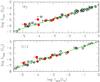 |
Fig. 9 Relationship between selected line luminosities and the accretion continuum luminosity. The red dots and arrows are the sample analyzed in this paper, the black asterisks refer to the sample analyzed by HH08, where they found the relation drawn as black line. The green solid line corresponds to the relation found using the actual detection of our sample as well. |
In Fig. 10 we show the correlation between Lacc,c and the Paβ line luminosity for the targets discussed in this paper, and for previous samples from the Ophiuchus and Cha I star-forming regions analyzed by Natta et al. (2004) and Muzerolle et al. (1998). The trend found by Natta et al. (2004) shows a good correlation over the whole range of masses from few tens of Jupiter masses to about one solar mass. Our new data confirm the trend found by Natta et al. (2004) and reinforce the strength of this line as an accretion indicator, agreeing with the results found by Antoniucci et al. (2011), who also tested the reliability of this indicator as accretion tracer.
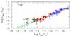 |
Fig. 10 Paβ luminosity as a function of Lacc,c. The black asterisks are the sample from Natta et al. (2004), the blue diamonds represent the sample analyzed by Muzerolle et al. (1998). The solid black line is the best-fitting relation found by Natta et al. (2004) (Eq. (2) of their paper). The green triangles are the objects of our sample, and the green line is the relation found combining these objects with the others. |
5.2.3. Other accretion tracers
A quite broad spread can be seen in Fig. 11 for the mass accretion rates retrieved using the CaII 866 nm line. We compared our results with those obtained by Mohanty et al. (2005) and HH08. Figure 11 shows their relationships. In particular, the black long-dashed line represents the linear fit of the data collected by Mohanty et al. (2005). These authors, moreover, suggested that there might be a small systematic offset between the higher mass accretors and the very low mass sample, with the latter possibly showing a somewhat higher CaII emission for a given Ṁacc. Consequently, Mohanty and collaborators performed separate fits for the higher and lower mass samples. Mohanty et al. (2005) speculated that the reason of this offset could lie in the methodology of Ṁacc derivation for the intermediate-mass objects (U-band veiling) with respect to the low-mass objects (Hα modeling), and/or in a different formation region of the CaII line in the two mass regimes (infalling gas or accretion shock).
We recomputed the relationship between Ṁacc and the flux of the CaII866 nm line (the green line in Fig. 11) considering the samples analyzed by Mohanty et al. (2005), HH08 and in this work (ignoring the upper limits). We find a flatter relationship with respect to those found by the other authors (see Table 8).
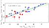 |
Fig. 11 Ṁacc,c versus flux of the CaII λ866.2 line. The blue triangles and the blue lines (long- and short-dashed) represent the data set and the correlation found by Mohanty et al. (2005). The black asterisk are the sample taken into account by HH08 and the blue dotted-dashed lines are the relationships found in their paper. The red points are the objects analyzed in this paper. The green solid line is the least square fit of all the targets plotted in the figure, neglecting the upper limits. |
Even though Ṁacc and the CaII 866 flux are correlated, the spread in flux for any given Ṁacc is broades than two orders of magnitude, and it is not trivial to decide which relation should be used to obtain an estimate of Ṁacc if the CaII 866 nm flux is known. This broad spread is partly due to the uncertainty in placing the continuum around the CaII Infra-Red Triplet (IRT) lines. We show in Fig. 12 the line profiles of this tracer in the sample analyzed here. In some cases (e.g. SO397 and SO646) the line emission is superposed on the absorption profile. This could cause an error in our estimate of the line fluxes. Moreover, as already noted by Mohanty et al. (2005), the CaII IRT lines are seen in emission only in accretors, but not all accretors show emission in these lines.
New relationships, including our sample, have also been computed for the CaIIλ854.2 nm line and NaIλ589.3 nm line, and are reported in Table 8.
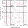 |
Fig. 12 CaII infra-red triplet line profiles of the class II objects. For each star three panels are presented: the left panel shows the CaIIλ849.8 nm line, the middle panel displays the CaIIλ854.2 nm line, and the CaIIλ866.2 nm line is shown in the right panel. |
Figure 13 shows the comparison between Lacc,c and the U-band photometric excess (LU). The U-band photometry for the X-shooter sample has been obtained by Rigliaco et al. (2011a) using FORS1 at the VLT, and thus is not simultaneous with the other accretion diagnostics analyzed since here. LU is highly correlated with Lacc,c, as also shown by Gullbring et al. (1998). With our sample we expand the relation to lower luminosities.
The new relationship is slightly different with respect to the relation found by Gullbring et al. (1998), and this is clearly due to the extension of the sample toward lower mass accretion rate regimes. These results confirm that, if the extinction can be estimated, or if it is negligible, as in the σ Orionis star-forming region, good accretion luminosities can be derived from the U-band photometry, also in low-accretion luminosity regimes.
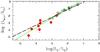 |
Fig. 13 Relation between the U-band brightness and total excess luminosity. The black asterisks refer to the sample analyzed by Gullbring et al. (1998), who found the relation drawn as dashed-black line. The red dots are the sample analyzed in this paper, and the green line is the relation found considering both samples together. |
5.3. Notes on some targets
We have seen in Sect. 5.1 that the accretion luminosity from the Balmer and Paschen excess continuum (Lacc,c) is within the 1σ uncertainty of the average accretion luminosity ( ⟨ Lacc,l ⟩ ) computed considering all secondary accretion indicators observed simultaneously, for five out of eight of the targets in our sample. Here we investigate the three sources where Lacc,c and Lacc,l are discrepant.
SO848: Lacc,c and ⟨ Lacc,l ⟩ differ by about a factor three. Looking at Fig. 6, we can easily see that for SO848 the estimates of Lacc,l from the CaII lines deviate from all other estimates. In the previous sections we have seen that the CaII lines are the most uncertain of the secondary accretion indicators, and that the estimate of the accretion luminosity strongly depends on the rate of accretion. If we neglect the accretion luminosity obtained from the CaII lines and recompute the average Lacc,l, we find that the discrepancy with Lacc,c becomes less than a factor two. These differences are within our uncertainty in the estimate of Lacc,c ( ⟨ log Lacc,l ⟩ neglecting the CaII points is ~−3.21).
SO1266: this object shows only a few features usable for deriving the accretion luminosities, and ⟨ Lacc,l ⟩ is the lowest of all values in our sample, while Lacc,c is only an upper limit. Young stellar objects are generally characterized by strong and intense chromospheric activity (see Fig. 14). This activity also produces hydrogen recombination lines, as well as the CaII H&K lines, among many others. We find that the Balmer series line of the class III objects is ~80% of the line luminosity of SO1266. This means that for this object, using the secondary accretion indicators, we are mainly tracing the chromospheric activity of the star, with only 20% of the line luminosities due to the accretion activity. The lack of a detectable accretion and the shape of the SED (see Fig. 1) suggest that the disk surrounding SO1266 is a transitional disk, in which the inner part is completely or nearly completely cleared of small dust but the outer disk is optically thick (Calvet et al. 2002; Cieza 2008). Note that Hernandez et al. (2007) did not include this object among their transitional disk candidates.
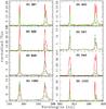 |
Fig. 14 Each panel shows the comparison between the target stars and the templates used to obtain the continuum accretion luminosity (as listed in Table 3) in the region of the CaII H (λ393.37 nm) and CaII K (λ396.85 nm) lines. The CaII K line is blended with the Hϵ at λ 397.0 nm. These lines are tracers of the chromospheric activity of the young stars. |
SO587: in this object there is no evidence of excess continuum emission, and the estimate of Lacc,c is an upper limit. This object has been already analyzed by Rigliaco et al. (2009). The star is most likely being photo-evaporated by the high-energy photons either from the central star or from the nearby hot star σOri.
One consideration to take into account in the analysis of the emission lines of this object is that the photoevaporative processes could produce some emission in the permitted lines, which, added to the chromospheric activity of the star, could be wrongly interpreted as due to accretion. However, this hypothesis still needs to be studied in depth, e.g., by analyzing higher resolution spectra in the regions where lines produced by photoevaporation are expected.
6. Summary
We have analyzed the broad-band, medium-resolution, high-sensitivity X-shooter spectra of a sample of young very low mass class II and class III stars in the σ Ori star-forming region. The sample was defined to cover the mass range ~0.08−~0.3 M⊙. We focused on the accretion properties of the class II stars, while class III stars were used only as spectral templates. We carried out a comparison between several accretion diagnostics observed simultaneously, that spanned from the UV excess continuum to the IR hydrogen recombination lines, computing the accretion luminosities and the mass accretion rates. We obtain the following results:
-
1.
We detected clear evidence of excess emission in the Balmercontinuum in six out of eight class II objects.Two of these also show hydrogen Paschen contin-uum emission. We estimated for all eight class IIsources the accretion luminosity from the excess contin-uum emission by fitting the observed continuum as the sumof the emission of a class III template andof a slab of hydrogen of varying density, temperature andlength, under the assumption of LTE and without taking intoaccount the contribution of the emission lines. We foundthat log Lacc,c rangesbetween ~−2.0 to ~−4.0 (L⊙) in the objects where the excess continuum is measured, which converts to a mass accretion rate Ṁacc in the range ~10-9 to ~5 × 10-11 M⊙/yr.
-
2.
We estimated the accretion luminosity from ten secondary accretion indicators using the empirical relationships with line flux and/or luminosity given in the literature. The accretion luminosities computed from all observable tracers show a dispersion around the average Lacc,l value of more than one order of magnitude, which cannot be explained by temporal variability given the simultaneous observation of all accretion tracers. This wide scatter may reflect a real spread in the values of the secondary indicators for fixed accretion luminosity, owing to, e.g., different stellar and/or disk properties, or differences in wind/jet contributions. We investigated the possibility that this spread may depend on the stellar masses or different regimes of mass accretion, and we found that these dependencies can be ruled out, agreeing with the results found by Curran et al. (2011) for higher mass objects. Despite this wide spread, for a given star all accretion luminosity indicators give values of Lacc,l, which are consistent within the error bars, and the average value of Lacc,l has a considerably reduced uncertainty, which is about a factor two. The average accretion luminosity from the secondary accretion indicators ( ⟨ log Lacc,l ⟩ ) ranges between ~ − 1.9 to ~−4.0 (L⊙), which converts in Ṁacc in the range ~ 2 × 10⁻⁹ to ~2 × 10-11 (M⊙/yr). Moreover, ⟨ log Lacc,l ⟩ is consistent with log Lacc,c obtained from the excess continuum emission.
-
3.
With respect to the reliability of the secondary accretion indicators, we found that in general the hydrogen recombination lines, spanning from the UV to the NIR, give good and consistent measurements of Lacc that often better agree than the uncertainties introduced by the adopted correlations. The average Lacc derived from several hydrogen lines, measured simultaneously, have a much reduced error. This suggests that some of the spread in the literature correlations may be due to the use of nonsimultaneous observations of lines and continuum, and that their quality will be significantly improved when a larger sample of X-shooter spectra will be available.
-
4.
We recomputed the relationships log Lacc – log Lline for the secondary accretion diagnostics used in this paper, combining our new data with those available in the literature. In most cases the relationships change only within the errors but in some cases (namely log Lacc − log LHα and log Lacc – log LCaII) the correlations change significantly when we include the low-accretion regime sampled in this paper. In particular, the correlation log Lacc – log LHα shows a flattening for log Lacc < ~ −3. This could be due to the increasingly important contribution coming from chromospheric activity for weak accretors. The correlation log Lacc – log LCaII shows a very big spread in log LCaII for any given log Lacc. As already noted by other authors (Muzerolle et al. 1998; Mohanty et al. 2005, HH08), this indicator could provide a very uncertain estimate of Lacc and/or Ṁacc. In general, a wider spread, as compared to the correlation with hydrogen lines, can be seen in the NaI line.
-
5.
The comparison between log Lacc,c and ⟨ log Lacc,l ⟩ obtained using the excess continuum emission and the emission line luminosities gives very encouraging results. The excess Balmer continuum accretion luminosities agree very well with the average ⟨ log Lacc,l ⟩ in five out of eight stars of our sample. The remaining three objects do not show such agreement. We discussed these three cases separately, finding that in each case the disagreement can be attributed to peculiar characteristics of the targets (strong wind caused by photoevaporation processes acting on SO587, wrong interpretation of the chromospheric activity for SO1266, and the large uncertainty of the CaII lines as accretion tracers for SO848). We conclude that the average accretion luminosity computed as the average of several secondary accretion indicators is as reliable as the accretion luminosity obtained from the excess continuum emission, except for peculiar cases.
Munich Image Data Analysis System.
IRAF is distributed by National Optical Astronomy Observatories, which is operated by the Association of Universities for Research in Astronomy, Inc., under cooperative agreement with the National Science Foundation.
The veiling rλ at wavelength λ is defined as (Fobs − Fphot)/Fphot where Fobs is the observed flux, and Fphot is the photospheric flux.
Acknowledgments
E.R. thanks Ilaria Pascucci for valuable discussions. The authors acknowledge C. Manara for helping with the class III targets. The authors are grateful to the ESO staff, in particular C. Martayan, for support in the observations, and P. Goldoni and A. Modigliani for their help with the X-shooter pipeline.
References
- Alcalá, J. M., Stelzer, B., Covino, E., et al. 2011, AN, 332, 242 [Google Scholar]
- Allard, F., Hauschildt, P., & Schweitzer, A. 2000, ApJ, 539, 366 [NASA ADS] [CrossRef] [Google Scholar]
- Antoniucci, S., Garcia Lopez, R., Nisini, B., et al. 2011, A&A, 534, 32 [Google Scholar]
- Baraffe, I., Chabrier, G., Allard, F., et al. 1998, A&A, 337, 403 [NASA ADS] [Google Scholar]
- Batalha, C. C., Stout-Batalha, N. M., Basri, G., & Terra, M. A. 1996, ApJS, 103, 211 [NASA ADS] [CrossRef] [Google Scholar]
- Béjar, V. J. S., Zapatero-Osorio, M. R., & Rebolo, R. 1999, ApJ, 521, 671 [NASA ADS] [CrossRef] [Google Scholar]
- Beristain, G., Edwards, S., & Kwan, J. 2001, ApJ, 551, 1037 [NASA ADS] [CrossRef] [Google Scholar]
- Briceño, C., Vivas, A. K., Calvet, N., et al. 2001, Science, 291, 93 [NASA ADS] [CrossRef] [Google Scholar]
- Brown, A. G. A., de Geus, E. J., & de Zeeuw, P. T. 1994, A&A, 289, 101 [NASA ADS] [Google Scholar]
- Caballero, J. A. 2008, MNRAS, 383, 750 [Google Scholar]
- Calvet, N., & Gullbring, E. 1998, ApJ, 509, 802 [NASA ADS] [CrossRef] [Google Scholar]
- Cieza, L. 2008, ASPC, 393, 35 [NASA ADS] [Google Scholar]
- Curran, R., Argiroffi, C., Sacco, G., et al. 2011, A&A, 526, 104 [Google Scholar]
- Cutri, R. M., et al. 2003, 2MASS All Sky Catalog of Point Sources, The IRSA 2MASS All-Sky Point Source Catalog, NASA/IPAC Infrared Science Archive (Pasadena, CA: NASA/IPAC), http://irsa.ipac.caltech.edu/application/Gator [Google Scholar]
- Dahm, S. E. 2008, AJ, 136, 521 [NASA ADS] [CrossRef] [Google Scholar]
- D’Alessio, P., Calvet, N., Hartmann, L., et al. 1999, ApJ, 527, 893 [NASA ADS] [CrossRef] [Google Scholar]
- De Zeeuw, P., Hoogerwerf, R., & de Bruijne, J. 1999, A&A, 117, 354 [Google Scholar]
- Edwards, S., Fischer, W., Hillenbrand, L., & Kwan, J. 2006, ApJ, 646, 319 [NASA ADS] [CrossRef] [Google Scholar]
- Fang, M., van Boekel, R., Wang, W., et al. 2009, A&A, 504, 461 [NASA ADS] [CrossRef] [EDP Sciences] [Google Scholar]
- Fedele, D., van den Ancker, M., Henning, T., et al. 2010, A&A, 510, 72 [Google Scholar]
- Fischer, W., Edwards, S., Hillendrand, L., & Kwan, J. 2011, ApJ, 730, 73 [NASA ADS] [CrossRef] [Google Scholar]
- Franchini, M., Morossi, C., & Malagnini, M. 1998, ApJ, 508, 370 [NASA ADS] [CrossRef] [Google Scholar]
- Franciosini, E., Pallavicini, R., & Sanz-Forcada, J. 2006, A&A, 446, 501 [NASA ADS] [CrossRef] [EDP Sciences] [Google Scholar]
- Gatti, T., Testi, L., Natta, A., et al. 2006, A&A, 460, 547 [NASA ADS] [CrossRef] [EDP Sciences] [Google Scholar]
- Gatti, T., Natta, A., Randich, S., et al. 2008, A&A, 481, 423 [NASA ADS] [CrossRef] [EDP Sciences] [Google Scholar]
- Gullbring, E., Hartmann, L., Briceno, C., & Calvet, N. 1998, ApJ, 492, 323 [NASA ADS] [CrossRef] [Google Scholar]
- Joy, A. H. 1945, ApJ, 102, 168 [NASA ADS] [CrossRef] [Google Scholar]
- Hartigan, P., Kenyon, S. J., Hartmann, L., et al. 1991, ApJ, 382, 617 [NASA ADS] [CrossRef] [Google Scholar]
- Hartigan, P., Edwards, S., & Ghandour, L. 1995, ApJ, 452, 736 [NASA ADS] [CrossRef] [Google Scholar]
- Hartmann, L., D’Alessio, P., Calvet, N., & Muzerolle, J. 2006, ApJ, 648, 484 [NASA ADS] [CrossRef] [Google Scholar]
- Herbst, W., Herbst, D. K., Grossman, E., & Weinstein, D. 1994, AJ, 108, 1906 [NASA ADS] [CrossRef] [Google Scholar]
- Herbst, E., Eistoffel, J., Mundt, R., & Scholz, A. 2007, in Protostars and Planets V, eds. B. Reipurth, D. Jewitt, & K. Keil (Tucson: Univ. Arizona Press), 297 [Google Scholar]
- Herczeg, G., & Hillenbrand, L. A. 2008, ApJ, 681, 594 [NASA ADS] [CrossRef] [Google Scholar]
- Herczeg, G., Linsky, J., Valenti, J., et al. 2002, ApJ, 572, 310 [NASA ADS] [CrossRef] [Google Scholar]
- Hernández, J., Hartmann, L., Megeath, S., et al. 2007, ApJ, 662, 1067 [NASA ADS] [CrossRef] [Google Scholar]
- Hauschildt, P., Allard, F., & Baron, E. 1999a, ApJ, 512, 277 [Google Scholar]
- Hauschildt, P., Allard, F., Ferguson, J., et al. 1999b, ApJ, 525, 871 [NASA ADS] [CrossRef] [Google Scholar]
- Hillenbrand, L., Strom, S., Calvet, N., et al. 1998, AJ, 116, 1816 [NASA ADS] [CrossRef] [Google Scholar]
- Houdebine, E., Mathioudakis, M., Doyle, J., & Foing, B. 1996, A&A, 305, 209 [NASA ADS] [Google Scholar]
- Jeffries, R. D., Maxted, P. F. L., Oliveira, J. M., & Naylor, T. 2006, MNRAS, 371, L10 [Google Scholar]
- Ingleby, L., Calvet, N., Hernández, J., et al. 2011a, AJ, 141, 127 [NASA ADS] [CrossRef] [Google Scholar]
- Ingleby, L., Calvet, N., Bergin, E., et al. 2011b, ApJ, 743, 105 [NASA ADS] [CrossRef] [Google Scholar]
- Kenyon, M. J., Jeffries, R. D., Naylor, T., et al. 2005, 356, 89 [Google Scholar]
- Köenigl, A. 1991, ApJ, 370, L39 [NASA ADS] [CrossRef] [Google Scholar]
- Luhman, K. L. 1999, ApJ, 525, 466 [NASA ADS] [CrossRef] [Google Scholar]
- Luhman, K., Stauffer, J., Muench, A., et al. 2003, ApJ, 593, 1093 [NASA ADS] [CrossRef] [Google Scholar]
- Mauas, P. J., & Falchi, A. 1996, A&A, 310, 245 [NASA ADS] [Google Scholar]
- Mohanty, S., Jayawardhana, R., & Basri, G. 2005, ApJ, 626, 498 [NASA ADS] [CrossRef] [Google Scholar]
- Muzerolle, J., Hartmann, L., & Calvet, N. 1998, AJ, 116, 455 [NASA ADS] [CrossRef] [Google Scholar]
- Muzerolle, J., Calvet, N., Briceño, C., Hartmann, L., & Hillenbrand, L. 2000, ApJ, 535, L47 [NASA ADS] [CrossRef] [PubMed] [Google Scholar]
- Muzerolle, J., Hillenbrand, L., Calvet, N., et al. 2003, ApJ, 592, 266 [NASA ADS] [CrossRef] [Google Scholar]
- Muzerolle, J., Luhman, K., Briceño, C., et al. 2005, ApJ, 625, 906 [NASA ADS] [CrossRef] [Google Scholar]
- Natta, A., Testi, L., Muzerolle, J., et al. 2004, A&A, 424, 603 [NASA ADS] [CrossRef] [EDP Sciences] [Google Scholar]
- Natta, A., Testi, L., & Randich, S. 2006, A&A, 452, 245 [NASA ADS] [CrossRef] [EDP Sciences] [Google Scholar]
- Oliveira, J., Jeffries, R., & van Loon, J. 2004, MNRAS, 347, 1327 [NASA ADS] [CrossRef] [Google Scholar]
- Pascucci, I., Sterzik, M., & Alexander, R. 2011, ApJ, 736, 13 [NASA ADS] [CrossRef] [Google Scholar]
- Perryman, M. A. C., Lindegren, L., Kovalevsky, J., et al. 1997, A&A, 323, L49 [NASA ADS] [Google Scholar]
- Riddick, F., Roche, P., & Lucas, P. 2007, MNRAS, 381, 1067 [NASA ADS] [CrossRef] [Google Scholar]
- Rigliaco, E., Natta, A., Randich, S., & Sacco, G. 2009, A&A, 495, L13 [NASA ADS] [CrossRef] [EDP Sciences] [Google Scholar]
- Rigliaco, E., Natta, A., Randich, S., et al. 2011a, A&A, 525, 47 [Google Scholar]
- Rigliaco, E., Natta, A., Randich, S., et al. 2011b, A&A, 526, 6 [Google Scholar]
- Rigliaco, E., Natta, A., Testi, L., et al. 2011c, AN, 332, 249 [NASA ADS] [Google Scholar]
- Rhode, K., Herbst, W., & Mathieu, R. 2001, AJ, 122, 3258 [NASA ADS] [CrossRef] [Google Scholar]
- Short, C. I., Doyle, J. G., & Byrne, P. B. 1997, A&A, 324, 196 [NASA ADS] [Google Scholar]
- Shu, F., Najita, J., Ostriker, E., & Wilkin, F. 1994, ApJ, 429, 781 [NASA ADS] [CrossRef] [Google Scholar]
- Telleschi, A., Güdel, M., Briggs, K., et al. 2007, A&A, 468, 443 [NASA ADS] [CrossRef] [EDP Sciences] [Google Scholar]
- Uchida, Y., & Shibata, K. 1985, PASJ, 37, 515 [NASA ADS] [Google Scholar]
- Valenti, J. A., Basri, G., & Johns, C. M. 1993, ApJ, 106, 2024 [Google Scholar]
- White, R., & Basri, G. 2003, ApJ, 582, 1109 [NASA ADS] [CrossRef] [Google Scholar]
- Yang, H., Herczeg, G., Linsky, J., et al. 2012, ApJ, 744, 121 [NASA ADS] [CrossRef] [Google Scholar]
- Zapatero Osorio, M. R., Béjar, V. J. S., Pavlenko, Y., et al. 2002, A&A, 384, 937 [NASA ADS] [CrossRef] [EDP Sciences] [Google Scholar]
All Tables
Line luminosity vs. accretion luminosity relationships for selected accretion indicators.
Newly determined line luminosity vs. accretion luminosity relationships for selected accretion indicators.
All Figures
|
Fig. 1 SEDs for the sample analyzed in this paper. Effective temperature of the adopted photospheric template is indicated as well as the name of the target. For all stars with excess above the photosphere, the median disk SED in Taurus (gray region) is displayed, scaled to the J-band flux. Black points are the photometric data (we did not apply any correction for the extinction because the reddening in the σOri star-forming region is negligible (Béjar et al. 1999; Oliveira et al. 2004)). |
| In the text | |
|
Fig. 2 Comparison between the observed spectra and the fit obtained considering the slab model. Red spectra represent the observed emission in the region of the Balmer jump after a smoothing by boxcar seven. The green spectra show the photospheric template, the cyan lines are the synthetic accretion spectra from the slab model. The sum of the slab model plus the template is shown by the blue spectra. |
| In the text | |
|
Fig. 3 Ca I λ422.6 nm absorption line in the X-shooter spectra (red-solid lines). The green line shows the spectrum of the adopted class III template and the blue-dashed line the adopted model with the emission predicted from the slab model added to the template. Fe I emission lines at 421.6, 422.7 and 423.3 nm can also be identified. |
| In the text | |
|
Fig. 4 Region around 700 nm. The red-solid lines shows the class II spectra, the green line shows the spectrum of the adopted class III template and the blue-dashed line the adopted model with the emission added to the template. |
| In the text | |
|
Fig. 5 Hα line profiles normalized at 700 nm (class II red lines, panel a), and class III cyan lines, panel b)). The class II line profiles exhibit diverse morphologies that presumably arise from differing accretion rate values, gas temperature, and geometries (inclinations and magnetospheric radii). |
| In the text | |
|
Fig. 6 Comparison between all accretion indicators listed in Table 6. The red dots are our estimates of the accretion luminosity, the red arrows are the upper limits, the yellow triangles refer to Lacc obtained from the U-band excess emission, which was observed non-simultaneously with the other indicators. The green dashed line is the average Lacc,l computed considering all secondary indicators; the green shaded region is the 1σ uncertainty in the average Lacc,l. The blue line is Lacc,c obtained using the excess continuum emission (dashed blue line for the upper limits). |
| In the text | |
|
Fig. 7 Comparison between the mass accretion rates computed from the average of all indicators (Ṁacc,l) and Ṁacc,c. |
| In the text | |
|
Fig. 8 Relationship between selected line luminosities and the accretion continuum luminosity. The red dots and arrows are the sample analyzed in this paper, the black asterisks and arrows refer to the sample analyzed by HH08. The gray crosses are the sample collected by Fang et al. (2009). The gray short-dashed line corresponds to the relation found by Fang et al. (2009). The black long-dashed line is the relation found by HH08, computed ignoring the upper limits in Lacc. The green lines correspond to the relations found using the actual detection of the sample analyzed here combined with the Fang et al. (2009) sample. |
| In the text | |
|
Fig. 9 Relationship between selected line luminosities and the accretion continuum luminosity. The red dots and arrows are the sample analyzed in this paper, the black asterisks refer to the sample analyzed by HH08, where they found the relation drawn as black line. The green solid line corresponds to the relation found using the actual detection of our sample as well. |
| In the text | |
|
Fig. 10 Paβ luminosity as a function of Lacc,c. The black asterisks are the sample from Natta et al. (2004), the blue diamonds represent the sample analyzed by Muzerolle et al. (1998). The solid black line is the best-fitting relation found by Natta et al. (2004) (Eq. (2) of their paper). The green triangles are the objects of our sample, and the green line is the relation found combining these objects with the others. |
| In the text | |
|
Fig. 11 Ṁacc,c versus flux of the CaII λ866.2 line. The blue triangles and the blue lines (long- and short-dashed) represent the data set and the correlation found by Mohanty et al. (2005). The black asterisk are the sample taken into account by HH08 and the blue dotted-dashed lines are the relationships found in their paper. The red points are the objects analyzed in this paper. The green solid line is the least square fit of all the targets plotted in the figure, neglecting the upper limits. |
| In the text | |
|
Fig. 12 CaII infra-red triplet line profiles of the class II objects. For each star three panels are presented: the left panel shows the CaIIλ849.8 nm line, the middle panel displays the CaIIλ854.2 nm line, and the CaIIλ866.2 nm line is shown in the right panel. |
| In the text | |
|
Fig. 13 Relation between the U-band brightness and total excess luminosity. The black asterisks refer to the sample analyzed by Gullbring et al. (1998), who found the relation drawn as dashed-black line. The red dots are the sample analyzed in this paper, and the green line is the relation found considering both samples together. |
| In the text | |
|
Fig. 14 Each panel shows the comparison between the target stars and the templates used to obtain the continuum accretion luminosity (as listed in Table 3) in the region of the CaII H (λ393.37 nm) and CaII K (λ396.85 nm) lines. The CaII K line is blended with the Hϵ at λ 397.0 nm. These lines are tracers of the chromospheric activity of the young stars. |
| In the text | |
Current usage metrics show cumulative count of Article Views (full-text article views including HTML views, PDF and ePub downloads, according to the available data) and Abstracts Views on Vision4Press platform.
Data correspond to usage on the plateform after 2015. The current usage metrics is available 48-96 hours after online publication and is updated daily on week days.
Initial download of the metrics may take a while.