| Issue |
A&A
Volume 548, December 2012
|
|
|---|---|---|
| Article Number | A82 | |
| Number of page(s) | 11 | |
| Section | Galactic structure, stellar clusters and populations | |
| DOI | https://doi.org/10.1051/0004-6361/201219750 | |
| Published online | 27 November 2012 | |
Chemical abundances in the old LMC globular cluster Hodge 11⋆,⋆⋆
1 Universidad de Concepción, Departamento de Astronomia, Fac. Cs. Físicas y Matemáticas. Barrio Universitario, Concepción, Chile
e-mail: This email address is being protected from spambots. You need JavaScript enabled to view it.
; This email address is being protected from spambots. You need JavaScript enabled to view it.
; This email address is being protected from spambots. You need JavaScript enabled to view it.
2 European Southern Observatory, Alonso de Cordova 3107, Vitacura, Santiago, Chile
e-mail: This email address is being protected from spambots. You need JavaScript enabled to view it.
3 Space Telescope Science Institute, 3700 San Martin Dr., Baltimore, MD 21218, USA
e-mail: This email address is being protected from spambots. You need JavaScript enabled to view it.
4 Department of Astronomy, University of Florida, Gainesville, FL 32611, USA
5 School of Mathematics & Physics, University of Tasmania, Private Bag 37, Hobart, TAS, Australia
6 National Optical Astronomy Observatories, PO Box 26732, Tucson, AZ 85726, USA
e-mail: This email address is being protected from spambots. You need JavaScript enabled to view it.
7 Dipartimento di Astronomia, Università di Padova, Vicolo Osservatorio 3, 35122 Padova, Italia
8 Astronomy Department, Yale University, New Haven, CT 06520, USA
Received: 4 June 2012
Accepted: 13 August 2012
Abstract
Context. The study of globular clusters is one of the most powerful ways to learn about a galaxy’s chemical evolution and star formation history. They preserve a record of chemical abundances at the time of their formation and are relatively easy to age date. The most detailed knowledge of the chemistry of a star is given by high resolution spectroscopy, which provides accurate abundances for a wide variety of elements, yielding a wealth of information on the various processes involved in the cluster’s chemical evolution.
Aims. We studied red giant branch (RGB) stars in an old, metal-poor globular cluster of the Large Magellanic Cloud (LMC), Hodge 11 (H11), in order to measure as many elements as possible. The goal is to compare its chemical trends to those in the Milky Way halo and dwarf spheroidal galaxies in order to help understand the formation history of the LMC and our own Galaxy.
Methods. We have obtained high resolution VLT/FLAMES spectra of eight RGB stars in H11. The spectral range allowed us to measure a variety of elements, including Fe, Mg, Ca, Ti, Si, Na, O, Ni, Cr, Sc, Mn, Co, Zn, Ba, La, Eu and Y.
Results. We derived a mean [Fe/H] = −2.00 ± 0.04, in the middle of previous determinations. We found low [α/Fe] abundances for our targets, more comparable to values found in dwarf spheroidal galaxies than in the Galactic halo, suggesting that if H11 is representative of its ancient populations then the LMC does not represent a good halo building block. Our [Ca/Fe] value is about 0.3 dex less than that of halo stars used to calibrate the Ca IR triplet technique for deriving metallicity. A hint of a Na abundance spread is observed. Its stars lie at the extreme high O, low Na end of the Na:O anti-correlation displayed by Galactic and LMC globular clusters.
Key words: stars: abundances / Magellanic Clouds / globular clusters: individual: Hodge 11
Based on observations collected at the European Organisation for Astronomical Research in the Southern Hemisphere, Chile (proposal ID 082.B-0458).
Table 4 is only available in electronic form at http://www.aanda.org
© ESO, 2012
1. Introduction
One of the most direct and powerful ways to learn about a galaxy’s chemical evolution and star formation history is through the study of its star clusters, which preserve a record of their galaxy’s chemical abundances at the time of their formation and are relatively easy to age date. Particularly important are the ancient globular clusters (GCs), which were witnesses to the construction of their parent galaxy. The most detailed knowledge of the chemistry of a star is given by high resolution spectroscopy (HRS), which provides accurate abundances for a wide variety of elements with a range of nucleosynthetic histories, yielding a wealth of information on the various processes involved in the cluster’s chemical evolution. The ages, kinematics, metallicities and abundance ratios derived from HRS of Galactic globular clusters (GGCs) have yielded a vast array of fascinating insights into their formation and that of the Milky Way.
With the advent of 8 m class telescopes equipped with multi-object HRS capability, such observations in the Large Magellanic Cloud (LMC) are now quite tractable. However, remarkably, despite the wealth of information that HRS of LMC star clusters could provide, only a handful of LMC GCs have been observed with HRS (Hill et al. 2000; Johnson et al. 2006, hereafter J06; Mucciarelli et al. 2009; Mucciarelli et al. 2010, hereafter M10). Such studies are desperately needed to tell us about the formation and early chemical evolution of our second nearest galactic neighbor, as well as that of our own Galaxy. Smaller galaxies like the LMC are often assumed to be the building blocks of larger galaxies in ΛCDM hierarchical formation models. However, detailed abundances in dwarf spheroidal (dSph) galaxies (e.g. Shetrone et al. 2001; Geisler et al. 2005) show that the abundances of giants in dSphs and dIrrs are quite distinct from those in the halo of the Milky Way. In particular, the dwarfs have depleted abundances of the α elements at a given [Fe/H] compared to their halo counterparts. This potentially serious problem for hierarchical formation models can be overcome, as suggested by Robertson et al. (2005), by assuming that the bulk of the halo was built by the accretion of only a very small number of very massive dwarfs (~LMC size) very early in the galaxy’s history. Such dwarfs would have had high star formation rates and fast chemical evolution, with enrichment dominated by Type II SNe, leading to high α abundances. In contrast, the dSphs we see today are low mass survivors, with low star formation rates and slower evolution and thus relatively depleted α abundances due to enrichment from both Types Ia and II SNe. An important test of their prediction is that the lowest metallicity stars in the LMC should follow similar abundance patterns to those in the halo. In particular, they should have enhanced [α/Fe] ratios. Only a tiny sample of such very metal-poor LMC stars have been studied in detail (Hill et al. 2000; Johnson et al. 2006; Pompéia et al. 2007), and results are inconclusive. Note that this problem may have been partly ameliorated by the recent discovery of two halo populations with distinct [α/Fe] ratios (Nissen & Schuster 2010). The high-α population is that normally associated with the halo, with a relatively constant value of [α/Fe] ~ 0.3, while the low-α population at the same [Fe/H] has [α/Fe] lower by an amount that increases with [Fe/H], from ~0.05 at [Fe/H] ~ −1.6 to ~ 0.15 at [Fe/H] ~ −0.8. However, in this same metallicity range, dSph stars have typical [α/Fe] values that are even lower, by ~0.1−0.3 dex (Geisler et al. 2007). This in fact leaves the bulk of the α problem intact.
In addition, previous large scale metallicity determinations for LMC clusters (Olszewski et al. 1991, hereafter O91; Grocholski et al. 2006, hereafter G06) have relied on using the Ca IR triplet as a proxy for measuring Fe abundances. This approach, however, has one potential flaw: it assumes that [Ca/Fe] is the same for the LMC as for the Galactic clusters used to calibrate the relationship. The very limited HRS studies available so far (Hill et al. 2000; Smith et al. 2002, J06; Pompéia et al. 2008, M10) have not yet arrived at a consistent, definitive picture in this regard. Further work is required to clarify and quantify the use of Ca as a proxy for Fe.
The LMC has some 13 known true GCs; i.e. clusters with ages and masses comparable to their Milky Way counterparts (Suntzeff et al. 1992). Given their significance delineated above, an HRS study of any of this sample would be of significant astrophysical importance. H11 is one such LMC GC. As such, and given its relatively uncrowded location, it has been the subject of a number of studies. Since the earliest CMD by its discoverer (Hodge 1960), it was suspected that H11 was a bonafide old cluster. Walker (1993, hereafter W93) showed that its very blue and bifurcated HB was similar to that of M15, and that it was very metal-poor, with [Fe/H] = −2.0 ± 0.2. Curiously, however, he did not find any RR Lyraes. Johnson et al. (1999) confirmed that H11 was as old as the oldest globulars in the Galaxy. The low metallicity found by W93 has been corroborated by all subsequent investigations, including low resolution blue (Cowley & Hartwick 1982) and IR Ca triplet (O91, G06) spectra and finally HRS. H11 was one of the first LMC GCs to be studied with HRS. In a pioneering study by J06, they not only observed H11 but also three other old LMC GCs. They used the MIKE spectrograph at the Magellan telescope to study two stars in H11.
Several years ago, our group began an independent HRS study of LMC star clusters similar to that of J06. Our motivation was to trace the chemical evolution of the LMC from its earliest beginnings and thus we necessarily required several old GCs. Despite the careful HRS study of J06, we felt a new investigation of H11 was warranted. First, J06 used the 6.5 m Magellan telescope, while we targeted the 8 m VLT. MIKE’s single slit allowed only one star to be observed at a time, and they only observed two stars, while we used the multiplexing capability of FLAMES to eventually observe eight members. Their resolution was 19 000, comparable to our GIRAFFE data, while our UVES data is a much higher 47 000. Their total exposure time was only 1 − 1.5 h while we integrated for a total of 7.5 h. They obtained abundances for 12 elements but these did not include Na, O, Al, Si, or Zn while we observed these five elements as well as their original 12. Na and O are particularly important given their almost ubiquitous anti-correlation in both GGCs (e.g. Carretta et al. 2009) as well as the few old, massive LMC GCs in which these elements have so far been studied (M10). Si, as one of the α elements, is also critical for examining such key issues as the Robertson et al. (2005)’s prediction.
J06 also found several results which sparked our interest in confirming or denying them. First, their metallicity of [Fe/H] = −2.21 ± 0.01 was lower than any other previous measurement, and 0.37 dex lower than the value we derived in our Ca triplet study (G06). Second, they found that, although the α element Mg was halo-like, both Ca and Ti were depleted with respect to the halo, at odds with M10. J06 suggested that the early chemical evolution of the LMC was significantly different from that of the halo, particularly with regards to the α elements, and more like that of dSphs, at odds with the Robertson et al. (2005)’s prediction and M10 findings for other LMC GCs.
Clearly, a more detailed investigation of H11 chemical abundances can address a number of outstanding issues. We present here our findings.
The paper is organized as follows: observations and reductions are given in Sect. 2. Section 3 presents the photometry performed, the estimation of atmospheric parameters and the abundance analysis. Results and a comparison with the literature are discussed in Sect. 4 and our major conclusions are summarized in Sect. 5.
Important parameters for our target stars.
2. Observations and data reduction
The observations were performed with the FLAMES (UVES+ GIRAFFE) spectrograph mounted on UT2 (Kueyen) at ESO-VLT Observatory in Paranal during January of 2009 (Proposal ID 082.B-0458). The GIRAFFE dataset was obtained using set-up H651.5A/HR14A (10 exposures of 45 min, wavelength range = 6308−6701 Å, R = 17 700). The selection of our targets was based on our study from G06, which confirmed metallicity and radial velocity membership for a number of giants. In addition we observed numerous field stars. GIRAFFE data were reduced using the ESO pipeline1. Data reduction includes bias subtraction, flat-field correction, wavelength calibration, sky subtraction, and spectral rectification. Spectra have a typical signal to noise (S/N) of ~50 at 6650 Å. Spectra of five of the brighter RGB stars were obtained with UVES using the 580 nm setting with 1.0′′ fibers, and cover the wavelength range 4800 − 6800 Å with a mean resolution of R = 47 000. UVES data were reduced using the UVES pipeline (Ballester et al. 2000), where raw data were bias-subtracted, flat-field corrected, extracted and wavelength calibrated. Finally, orders were merged to obtain a 1D spectrum and for each star the 10 × 45 min. exposure sky-subtracted spectra were combined to obtain the final spectrum for the analysis (see Fig. 1 for an example). The mean S/N is 25 per resolution element at 6650 Å.
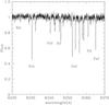 |
Fig. 1 Detailed view of our best UVES spectrum, TARG.6, in the range of 6220 − 6270 Å. Several important lines are identified. |
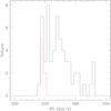 |
Fig. 2 Velocity histogram for GIRAFFE and UVES data. In red are the Hodge 11 members. There were three additional stars with RVs very close to that of the cluster, but the spectra showed many more lines, therefore their metallicities are much higher, and they were considered field stars. |
Membership was established by radial velocity (RV) measurement. We used the fxcor IRAF2 utility to measure RVs for both sets of data (GIRAFFE and UVES). This routine cross-correlates the observed spectrum with a template, in our case a synthetic spectrum with the mean atmospheric parameters of our targets (effective temperature (Teff) = 4600 K, surface gravity (log g) = 1.5, microturbulence velocity (vt) = 1.6 km s-1, metallicity ([m/H]) = −2.0). For the 101 stars observed with GIRAFFE we found a total of seven stars with RV comparable to the mean H11 RV value from G06 (RV = 245.1 ± 0.3 km s-1 and σRV = 1.0 km s-1), but only four of them were finally selected as H11 members. The other three stars have a completely different metallicity (as revealed by the numerous strong FeI lines in their spectra). From the UVES data, four stars have a RV and metallicities comparable to the values of H11 from G06. The final analysis thus gives a total of eight members for our cluster. A histogram of RVs is shown in Fig. 2. From the measured RVs we obtained a mean heliocentric ⟨RV⟩H = 245.9 ± 0.9 km s-1 and a dispersion σ ⟨RV⟩ = 2.5 km s-1.
Finally, for the abundance analysis, each spectrum was shifted to rest-frame velocity and continuum-normalized. Table 1 lists the basic parameters of the observed stars: the ID, the J2000.0 coordinates (RA and Dec), radial velocity (RV), V magnitude, (V − I) colors (from our own photometry), Teff, microturbulence velocity (vt), surface gravity (log g), and the typical signal to noise (S/N).
3. Photometry and abundance analysis
3.1. Photometry
For the determination of the atmospheric parameters we used photometric results from observations we performed at Las Campanas Observatory. We obtained images in V and I filters using the SITe#3 CCD camera mounted on the Swope 1.0 m telescope.
The images were pre-reduced using IRAF tasks for bias, linearity (based on the recipe discussed in Hamuy et al. 2006) and flat field corrections. The photometry was performed using the IRAF DAOPHOT/ALLSTAR and PHOTCAL packages. Instrumental magnitudes were extracted following the point-spread function (PSF) method (Stetson 1987). A quadratic, spatially variable, master PSF (PENNY function) was adopted because of the large field of view of the detector. Aperture corrections were then determined performing aperture photometry of a suitable number (typically 15 to 20) bright, isolated stars in the field. These corrections were found to vary from 0.160 to 0.290 mag, depending on the filter. The PSF photometry was finally aperture corrected, filter by filter. The calibration was done using standard field SA98 (Landolt 1992) with approximately 20 standard stars in the field. The final rms of the fit to the standards was 0.032 and 0.033 for V and I filters, respectively. At the mean magnitude of our targets, the internal error in V magnitude is 0.025 and 0.029 in (V − I) color for our Swope data.
A previous set of images for H11 were obtained using VLT/FORS2 during the course of the preimages obtained for the spectroscopic study by G06 and we reduced this data as well. The photometry procedure was the same as above. The results were calibrated using published photometry from W93. A color − magnitude diagram of H11 is shown in Fig. 3 using both photometric datasets. The FORS2 data is much deeper than the Swope data but the brightest stars appear saturated, including some of our targets. This was the main reason to use the Swope photometry and not FORS2 in our analysis. The mean difference, without regard to sign, between the Swope and FORS2 photometry around the RGB is ΔV = +0.1 and Δ(V − I) = +0.025. We decided to use the Swope data for our stars except for TARG.2, because in the 1.0 m photometry it is contaminated by another star.
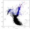 |
Fig. 3 Color–magnitude diagram for H11. Black dots: photometry from FORS2(VLT) pre-images from G06. Blue triangles: our data from the Swope Telescope at Las Campanas Observatory. H11 stars observed spectroscopically in this study are shown in red triangles (Swope data) and red dot (FORS2 data). |
3.2. Abundance analysis
Effective temperature was derived from the (V − I) color using the relation by Alonso et al. (1999) and the reddening (E(B − V) = 0.08) from W93. Surface gravities (log g) were obtained from the canonical equation: 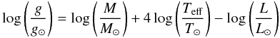 (1)where the mass M/M⊙ was assumed to be 0.8 M⊙, and the luminosity L/L⊙ was obtained from the absolute magnitude MV assuming a true distance modulus of (m − M)0 = 18.5 from Gieren et al. (2005). The bolometric correction (BC) was derived by adopting the relation BC − Teff from Alonso et al. (1999). Finally, microturbulence velocity (vt) was obtained from the relation vt − log g used in Marino et al. (2008) for the same type of stars as in our sample. Because of H11’s low metallicity and the relatively low signal to noise of our spectra, we used the spectrum-synthesis method to derive abundances for all the elements. For this purpose we calculated five synthetic spectra (Fig. 4) with different abundances for each element, and interpolated to derive the value that minimizes the rms of the fit. The local thermodynamic equilibrium (LTE) program MOOG (Sneden 1973) was used for the abundance analysis. The line list used, based on Villanova et al. (2009), is shown in Table 4. In the case of Mn we included hyperfine structure and for Ba we used solar isotopic ratios. In column two of Table 4 we adopt the MOOG notation (two-digit designation to the left of the decimal point, and a single digit to the right of the decimal point to represent the ionization stage, where zero denotes neutral and one denotes singly ionized) and in parentheses we denote the different isotopes used in the case of Ba. Atmospheric models by Kurucz (1970) were utilized and non-LTE corrections were made for Na lines based on Mashonkina et al. (2000). The solar abundances used are from Villanova et al. (2009).
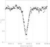 |
Fig. 4 Example of the spectral synthesis method. Five different spectra, with Fe abundance varying from 5.12 to 5.52, are shown fitted to the data in the measurement of a line of FeI (6335.3 Å) in TARG.6. |
Errors in [X/Fe] for stellar parameters.
3.3. Error analysis
The calculation of the effect of internal errors on the determination of the abundances was made varying the atmospheric parameters in the following way: ΔTeff = +50 K (based on the error in (V − I)), Δlog g = +0.10 (using the variation of +50 K in Teff and the error in magnitude V in the canonical equation), Δvt = +0.05 (from the variation in log g) and Δ[m/H] = + 0.1 (from our dispersion (σobs) in [Fe/H]), and recalculating the abundances for TARG.4, assumed to be representative of our sample. These values can be easily rescaled to different errors in each atmospheric parameter if necessary. The value of σS/N for one line is the mean of the rms of the Fe abundance measurements per star, which is 0.06 dex. To obtain the error in S/N for a given element and a given star, we divided this value by the square root of the number of lines used for that element.
The resulting errors for each [X/Fe]3 ratio due to uncertainties in each atmospheric parameter are listed in Table 2. The value of σtot was given by: ![Mathematical equation: \begin{eqnarray} \sigma_{\rm tot}=\sqrt{\sigma_{T_{\rm eff}}^{2} +\sigma_{\log g}^{2} + \sigma_{v_{\rm t}}^{2} + \sigma_{\rm [m/H]}^{2} + \sigma_{\rm S/N}^{2}}. \end{eqnarray}](/articles/aa/full_html/2012/12/aa19750-12/aa19750-12-eq95.png) (2)The total internal error for each element is also compared to the observed error (standard deviation of the sample) in Table 2.
(2)The total internal error for each element is also compared to the observed error (standard deviation of the sample) in Table 2.
4. Results
All results for the abundances of the different chemical species for our eight members of Hodge 11 are presented in Table 3. In parentheses we give the number of lines used.
[X/Fe] values for Hodge 11 stars.
4.1. Fe-peak elements
The mean value of [Fe/H] from our eight cluster members is: ⟨[Fe/H]⟩ = −2.00 ± 0.04 and σobs = 0.11 ± 0.03, with no evidence for any intrinsic variation. J06 give values of − 2.21 ± 0.01 (FeI) and − 2.05 ± 0.06 (FeII) from their two stars. Their FeI value is significantly lower than ours (also obtained with FeI), while their FeII value is comparable to our FeI value. Two previous studies employed the Ca triplet technique (CaT) to derive the mean metallicity of H11. O91 observed two stars, finding [Fe/H] = −2.06 ± 0.2 while G06 derived a mean of − 1.84 ± 0.04 (internal error only) from 12 giants. Our value agrees well with the former and is significantly lower than that of the latter. Photometrically, W93 found a value of [Fe/H] = − 2.0 ± 0.2, the same as ours. H11 clearly remains one of the LMC’s most metal-poor constituents.
The mean values for the other iron-peak elements are ⟨[Sc/Fe]⟩ = 0.07 ± 0.09, σobs = 0.16 ± 06, ⟨[Cr/Fe]⟩ = −0.49 ± 0.01, σobs = 0.02 ± 0.08 and ⟨[Ni/Fe]⟩ = −0.16 ± 0.05, σobs = 0.13 ± 0.04. We present our results for these iron-peak elements in comparison with the literature data in Fig. 5. In addition, we derive [Mn/Fe] = −0.49 and [Co/Fe] = 0.26 from a single (albeit our best UVES) star. Our results are in excellent agreement with those of J06 for Sc and Ni, while the accord is reasonable for both Mn and Co. However, our results show a very low abundance in [Cr/Fe] compared to J06 and to halo stars. Venn et al. (2012) also found a low value for Cr in Carina metal poor stars. This could be explained as a lack of high energy SNeII in the environment of the protocluster. Possibly these stars did not form or their gas was removed by SNe-driven winds (Umeda & Nomoto 2002).
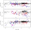 |
Fig. 5 Abundances for iron peak elements. Magenta dots are our results for Hodge 11, in red the LMC data: triangles correspond to J06, open circles correspond to Pompéia et al. (2008), stars correspond to Mucciarelli et al. (2008) and M10. In black dots Galaxy data from Fulbright (2000), Lee & Carney (2002), Cayrel et al. (2004) and Reddy et al. (2006), in blue squares data of dSph galaxies from Shetrone et al. (2001) and Sbordone et al. (2007). Error bar stands for σtot from Table 2. |
J06 found an even lower value, − 0.67, for Mn. They also found a low abundance for [V/Fe] in their other clusters, reminiscent of our Cr and both Mn values for H11. We have no explanation for the Cr difference with J06, but note that our three stars all give very similar values. We generally confirm what J06 found: Fe-peak elements in LMC clusters are relatively depleted or even strongly depleted in the case of Cr and Mn, and comparable to the values of dSph stars, although the latter data are sparse.
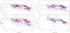 |
Fig. 6 Abundances for α-elements compared to the literature. Magenta dots are our results for Hodge 11, in red the LMC data: triangles correspond to J06, open circles correspond to Pompéia et al. (2008), stars correspond to Mucciarelli et al. (2008) and M10. In black dots Galaxy data from Fulbright (2000) and Lee & Carney (2002), in blue squares data of dSph galaxies from Shetrone et al. (2001), Sbordone et al. (2007) and Monaco et al. (2005). Error bar stands for σtot from Table 2. |
4.2. α-elements
The mean abundances for the main alpha-elements are ⟨[Mg/Fe]⟩ = 0.25 ± 0.06 and σobs = 0.12 ± 0.04, ⟨[Si/Fe]⟩ = 0.39 ± 0.06 and σobs = 0.11 ± 0.04, ⟨[Ca/Fe]⟩ = 0.13 ± 0.04 and σobs = 0.10 ± 0.03 and ⟨[Ti/Fe]⟩ = 0.16 ± 0.03 and σobs = 0.06 ± 0.02. The respective values from J06 are ⟨[Mg/Fe]⟩ = 0.46 ± 0.02, ⟨[Ca/Fe]⟩ = 0.30 ± 0.03 and ⟨[Ti/Fe]⟩ = −0.04 ± 0.05 (they did not measure Si).
Figure 6 shows our results for the α element ratios in comparison with the literature, in particular J06, M10 and halo stars. The agreement with J06 is fair. In the case of Mg we get a lower value than J06, M10 and halo stars. J06 got a value in agreement with the abundance of halo stars for H11, but the other GCs in their study show lower Mg values. M10 found values for their GCs comparable to the halo with some slightly lower values. We observe in our results a dispersion in Mg. Venn et al. (2012) suggest that this dispersion could possibly be due to inhomogeneous mixing of the interstellar gas.
For Si J06 has no data, but their other GCs lie on the halo trend, as do the mean of M10 clusters. Our results are slightly low in comparison to halo stars. We show a particularly low abundance in [Ca/Fe], confirming the J06 results for other GCs but not for H11, for which they find an abundance 0.17 dex higher than we do. M10, on the other hand, find halo-like Ca abundances in their sample.
If our low Ca abundance is correct, this could portend a serious problem for the CaT technique, which assumes that [Ca/Fe] is the same for the LMC as for the Galactic clusters used to calibrate the Ca to Fe relationship. Our [Ca/Fe] value is about 0.3 dex less than that of halo stars used to calibrate the CaT technique. Thus, CaT, applied to H11 but using Galactic calibrators, should derive a relatively metal-poor metallicity compared to its actual [Fe/H]. This difference, however, is in the opposite sense to that required to explain the offset between our [Fe/H] value and that derived by G06 from CaT. However, it is not clear that the Ca triplet metallicities should scale in an obvious way with [Ca/Fe]. Also, to properly address this issue would require analysing a sample of GGCs using the same techniques and solar abundances as adopted in our analysis of H11. Pompéia et al. (2008) found that there was no real correlation between the Ca triplet metallicities, FLAMES high-resolution [Fe/H], and [Ca/Fe] for a large LMC field star sample. This may have to do with the continuum level around the Ca triplet lines, which is set by H-ions, whose abundance is controlled much more by α-elements and sodium than it is by the Fe abundance. There is also a complication that the Ca triplet abundances are determined using a V magnitude, and if the α elements are very different, then the stellar colors will shift, changing V for a given bolometric luminosity. In any case, any shift empirically seems to be small.
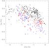 |
Fig. 7 Mean [α/Fe] abundance ratio vs. [Fe/H]. Same symbols and colors as in Fig. 6 with the addition of Nissen & Schuster (2010) high- and low-α halo stars (black open circle). |
Our Ti abundance is 0.2 dex higher than that of J06, who found their value, which was slightly subsolar, substantially lower than halo stars at the same metallicity. They found a similar result for their other GCs. Our value is only slightly lower than the halo mean and in good agreement with M10 values.
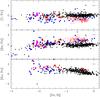 |
Fig. 8 Neutron-capture element abundances. Magenta dots are our results for Hodge 11, in red the LMC data: triangles correspond to J06, open circles correspond to Pompéia et al. (2008), stars correspond to Mucciarelli et al. (2008) and M10. In black dots Galaxy data from Fulbright (2000), Lee & Carney (2002), Reddy et al. (2003, 2006), in blue squares data of dSph galaxies from Shetrone et al. (2001) and Sbordone et al. (2007). Error bars stands for σtot from Table 2. |
Given the limitations of only a few lines in a small number of stars, and the similar nucleosynthetic genesis of these elements, the best metric is to derive the mean α abundance for all four elements. Unfortunately, we have all four elements in only three stars. The mean [α/Fe] ratio vs. [Fe/H] is plotted in Fig. 7, along with the equivalent data for J06 and M10 GC, LMC field stars from Pompéia et al. (2008), Galactic data from Fulbright (2000), Cayrel et al. (2004), Lee & Carney (2002) and Nissen & Schuster (2010), and dSphs data from Shetrone et al. (2001), Sbordone et al. (2007) and Monaco et al. (2005). This diagram is an excellent diagnostic for separating out halo from dSph stars, especially at the more metal-rich end (e.g. Geisler et al. 2007), as is clearly seen. Note that the Nissen & Schuster (2010) low-α stars are indeed a lower envelope to the halo distribution and that dSph stars are normally at significantly lower [α/Fe] for the same metallicity. According to the Robertson et al. (2005) scenario, the halo was mainly built up by the merger of only a few very massive dwarfs with LMC-like masses, with fast evolutionary timescales and thus enhanced [α/Fe] ratios from SNeII. The dSphs we see today are much lower mass survivors, who experienced much slower star formation rates which allowed SNIa to eventually contribute their ejecta, leading to depleted [α/Fe] ratios at higher metallicities. Where does the LMC fit into this diagram? Looking at the M10 data yields the clear impression that, at least at metallicities up to about − 1.6, the LMC does indeed overlap well with the halo. However, all other LMC data, including J06 GCs and the Pompéia et al. (2008) field stars, as well as our three H11 stars, indicate that, even at the low metallicity of H11, the LMC was already showing SNe Ia depletion effects, mimicking the dSphs. This depletion compared to the halo continues to grow with metallicity, becoming quite severe by [Fe/H] = − 1. The overall impression, then, is that the LMC is more dSph-like than halo-like in this diagram, confirming what J06 pointed out and in contradiction to M10 findings and Robertson et al. (2005) prediction.
4.3. Neutron capture elements
[Ba/Fe], [Y/Fe] and [Eu/Fe] abundances for H11 are shown in Fig. 8 in comparison with literature data for the Galaxy halo, dSphs and LMC GCs and field stars. The average abundance for each neutron capture element is ⟨[Y/Fe]⟩ = 0.04 ± 0.08 and σobs = 0.14 ± 0.06, ⟨[Ba/Fe]⟩ = −0.01 ± 0.08 and σobs = 0.23 ± 0.06 and ⟨[Eu/Fe]⟩ = 0.62 ± 0.04 and σobs = 0.05 ± 0.02.
Our results are in good agreement with J06 for both Y and Ba. However, it is difficult to make a distinction between the Galactic halo and the dSph locus at this metallicity. In [Ba/Fe] we have particularly good agreement with M10 results.
On the other hand, our [Eu/Fe] abundance is lower than J06 for H11 and again is comparable to M10 results, a little higher than Galactic halo stars. We obtained a value of log ε (La/Eu) of 0.07, which places the cluster in the r-process only region, according to Sneden et al. (2008) (Fig. 12a). This means that the cluster was formed from material polluted by SNe only, with no contribution from AGB stars, similar to the most metal poor stars of our Galaxy ([Fe/H] < −3.0, Sneden et al. 2008). In Fig. 9 the [Ba/Y] ratio vs. [Fe/H] shows H11 falls in the same region as both Galactic and dSph stars. One clearly sees that both Galactic and dSph stars share the same low metallicity trend, with the [Ba/Y] ratio increasing as metallicity increases until approximately [Fe/H] = −2.0, the metallicity of H11. At higher metallicity, the LMC and dSph stars separate from the Galaxy. This can be observed in Fig. 9 where LMC data from other authors, in red, are included. Colucci et al. (2012) claim that the LMC has undergone much slower star formation than the Galaxy, based on the fact that for the LMC the [Ba/Y] ratio increases with decreasing age and with increasing metallicity above −2. In addition, we show in Fig. 10 the [Ba/Eu] ratio vs. [Fe/H], our H11 data in magenta, LMC data in red, Galactic data in black and dSphs in blue. H11 clearly falls in the r-process regime, given that [Ba/Eu] has been used as a test for the s- or r-origin of these elements (Sneden et al. 1997).
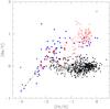 |
Fig. 9 [Ba/Y] ratio vs. [Fe/H] for H11 in magenta dots; Galactic data in black: dots from Fulbright (2000) and open circles from Nissen & Schuster (2011), blue squares are dSph data from Shetrone et al. (2001) and Shetrone et al. (2003), LMC data in red: triangles are J06, stars are old GCs from M10 and intermediate age clusters from Mucciarelli et al. (2008), open circles from Pompéia et al. (2008). The segmented line shows the Galactic trend. |
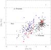 |
Fig. 10 [Ba/Eu] ratio vs. [Fe/H] for H11 in magenta dots; Galactic data in black dots from McWilliam et al. (1995), Reddy et al. (2003, 2006), Burris et al. (2000), Fulbright (2000), blue squares are dSph data (Shetrone et al. 2001; Shetrone et al. 2003; Geisler et al. 2005), LMC data in red: triangles are J06, stars are old GCs from M10 and intermediate age clusters from Mucciarelli et al. (2008). |
4.4. Na and O
In order to study the Na and O content in H11 compared to Galactic (Carretta et al. 2009) and LMC GCs (Mucciarelli et al. 2008), we present the abundances of [Na/Fe] and [O/Fe] in Fig. 11. Unfortunately, our data is limited to only three stars. The mean value in H11 for [Na/Fe] = −0.32 ± 0.07, σobs = 0.14 ± 0.05 and for [O/Fe] = 0.54 ± 0.03, σobs = 0.05 ± 0.02. H11 stars present a low [Na/Fe] abundance, confirming J06’s suggestion that LMC stars were probably born with low [Na/Fe]. A very high [O/Fe] abundance is shown in Fig. 11 for our stars. They stand at the extreme end of the trend of the anti-correlation displayed by GGCs. From the comparison of σobs and our total internal error, we find a hint of a spread in the Na abundance, but more data is needed to confirm this. No O spread is visible, but this is expected at the position of our stars in the Na:O relation.
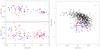 |
Fig. 11 Left: [Na/Fe] and [O/Fe] vs. [Fe/H], right: [Na/Fe] vs. [O/Fe] showing the Na:O anti-correlation in GCs. Magenta dots are our results for H11, in red other LMC data: triangles are results from J06, open circles are results from Pompéia et al. (2008), stars are results from Mucciarelli et al. (2008) and M10; in black filled circles are GGC data from Carretta et al. (2009) and Lee & Carney (2002), in blue squares dSph galaxies from Shetrone et al. (2001), Sbordone et al. (2007) and Monaco et al. (2005). Error bars stands for σtot from Table 2. |
5. Summary and conclusions
We determined for H11 a metallicity of [Fe/H] = −2.00 ± 0.04 and σobs = 0.11 ± 0.03, confirming it as one of the most metal poor clusters in the LMC (O91; W93; J06). G06 found a higher value using the CaT technique. We found that [Ca/Fe] is significantly lower than Galactic halo calibrators, so that CaT might be expected to give a relatively low, not high, metallicity. J06 also obtained low values of Ca in their study. However, M10 found values comparable to the Galaxy in their sample of three other old LMC GCs. Clearly, more investigation is need to clarify the appropriateness of using Ca as a proxy for Fe.
One of the most important results in this study is that from the mean [α/Fe] vs. [Fe/H] plot (Fig. 7). We find that H11 lies in the range of the dSph trend and below the Galactic one. This result confirms J06 and opens the possibility that galaxies like the LMC, assumed to be building blocks of our galaxy (from ΛCDM hierarchical formation models), may not in fact satisfy the chemical requirements, even at the low metallicity represented by H11. In the iron-peak elements, we also see abundance similarities to the dSph results, such as low Cr, Mn and Ni.
Another interesting result has to do with observational constraints on the masses of SNII progenitors from relative abundances, especially of the alpha elements. We have found low values for Mg, Ca and Ti, as did Venn et al. (2012) in Carina metal-poor stars. The yields of these elements (Ca and Mg in particular) depend on the progenitor SNe mass. Assuming that Woosley & Weaver (1995) reflects reality to first order, a high [O/Mg] abundance could indicate preferential pollution from 15 − 25 M/M⊙ SNeII (at least for Solar metallicities, Gibson 1997). In addition, Eu is an indicator of the r-process (main source: 8 − 10 M/M⊙ stars) and in our results the Eu abundance is high, indicating lower mass progenitors (Woosley & Weaver 1995).
A hint of a Na spread is suggested by comparing the σobs value with our internal errors (see Table 2). This spread is normal at the position of our targets in their location in the GGC Na:O trend. H11 presents a behavior similar to that of intermediate-age LMC clusters from Mucciarelli et al. (2008) shown in Fig. 11, with the hint of a Na but no O spread. The difference in the O abundance between Mucciarelli et al. (2008) sample and our data resides in the fact that the environment where H11 was formed was α-enhanced. Our data fall in the extreme high O, low Na end of the Na:O anti-correlation trend (see Fig. 11). H11 is only slightly less massive (Mackey & Gilmore 2003) than the three old LMC GCs found by M10 to follow the same Na:O anticorrelation as GGCs, and more massive than the intermediate-age LMC clusters from Mucciarelli et al. (2008) which show a hint of anticorrelation.
Finally, our result for [La/Eu] shows that these neutron capture elements were formed totally by the r-process, implying SNe-only pollution, without the influence of AGB stars.
Online material
Line list used.
IRAF is distributed by the National Optical Astronomy Observatory, which is operated by the Association of Universities for Research in Astronomy, Inc., under cooperative agreement with the National Science Foundation.
Where X corresponds to any chemical species.
Acknowledgments
R.M. would like to thank Brad K. Gibson for his comments on the paper, CONICYT (Chile) for a Ph.D. scholarship and the European Southern Observatory (ESO) for the experience to serve as a Ph.D. student in the Santiago de Chile offices. D.G. and S.V. gratefully acknowledge support from the Chilean BASAL Centro de Excelencia en Astrofisica y Tecnologias Afines (CATA) grant PFB-06/2007.
References
- Alonso, A., Arribas, S., & Martínez-Roger, C. 1999, A&AS, 140, 261 [NASA ADS] [CrossRef] [EDP Sciences] [Google Scholar]
- Ballester, P., Modigliani, A., Boitquin, O., et al. 2000, The Messenger, 101, 31 [NASA ADS] [Google Scholar]
- Burris, D., Pilachowski, C. A., Armandroff, T. E., et al. 2000, ApJ, 544, 302 [NASA ADS] [CrossRef] [Google Scholar]
- Carretta, E., Bragaglia, A., Gratton, R. G., et al. 2009, A&A, 505, 117 [NASA ADS] [CrossRef] [EDP Sciences] [Google Scholar]
- Cayrel, R., Depagne, E., Spite, M., et al. 2004, A&A, 416, 1117 [NASA ADS] [CrossRef] [EDP Sciences] [Google Scholar]
- Cowley, A. P., & Hartwick, F. D. A. 1982, ApJ, 259, 89 [NASA ADS] [CrossRef] [Google Scholar]
- Colucci, J. E., Bernstein, R. A., Cameron, S. A., & McWilliam, A. 2012, ApJ, 746, 29 [NASA ADS] [CrossRef] [Google Scholar]
- Fulbright, J. 2000, AJ, 120, 1841 [NASA ADS] [CrossRef] [Google Scholar]
- Geisler, D., Smith, V. V., Wallerstein, G., Gonzalez, G., & Charbonnel, C. 2005, AJ, 129, 1428 [NASA ADS] [CrossRef] [Google Scholar]
- Geisler, D., Wallerstein, G., Smith, V. V., & Casetti-Dinescu, D. I. 2007, PASP, 119, 939 [NASA ADS] [CrossRef] [Google Scholar]
- Gibson, B. K. 1997, MNRAS, 290, 471 [NASA ADS] [Google Scholar]
- Gieren, W., Storm, J., Barnes, T. G., III, et al. 2005, ApJ, 627, 224 [NASA ADS] [CrossRef] [Google Scholar]
- Grevesse, N., & Sauval, A. J. 1998, SSRv, 85, 161 [Google Scholar]
- Grocholski, A. J., Cole, A. A., Sarajedini, A., Geisler, D., & Smith, V. V. 2006, AJ, 132, 1630 [NASA ADS] [CrossRef] [Google Scholar]
- Hamuy, M., Folatelli, G., Morrell, N. I., et al. 2006, PASP, 118, 2 [NASA ADS] [CrossRef] [Google Scholar]
- Hill, V., François, P., Spite, M., Primas, F., & Spite, F. 2000, A&A, 364, L19 [NASA ADS] [Google Scholar]
- Hodge, P. W. 1960, ApJ, 131, 351 [NASA ADS] [CrossRef] [Google Scholar]
- Johnson, J. A., Bolte, M., Stetson, P. B., Hesser, J. E., & Somerville, R. S. 1999, ApJ, 527, 199 [NASA ADS] [CrossRef] [Google Scholar]
- Johnson, J. A., Ivans, I. I., & Stetson, P. B. 2006, ApJ, 640, 801 [NASA ADS] [CrossRef] [Google Scholar]
- Kurucz, R. L. 1970, SAO Special Report, 309 [Google Scholar]
- Landolt, A. U. 1992, AJ, 104, 340 [NASA ADS] [CrossRef] [Google Scholar]
- Lee, J.-W., & Carney, B. W. 2002, AJ, 124, 1511 [NASA ADS] [CrossRef] [Google Scholar]
- Mackey, A. D., & Gilmore, G. F. 2003, MNRAS, 338, 85 [NASA ADS] [CrossRef] [Google Scholar]
- Marino, A. F., Villanova, S., Piotto, G., et al. 2008, A&A, 490, 625 [NASA ADS] [CrossRef] [EDP Sciences] [Google Scholar]
- Mashonkina, L. I., Shimanski, V. V., & Sakhibullin, N. A. 2000, Astron. Rep., 44, 790 [NASA ADS] [CrossRef] [Google Scholar]
- McWilliam, A., Preston, G. W., Sneden, C., & Shectman, S. 1995, AJ, 109, 2736 [NASA ADS] [CrossRef] [Google Scholar]
- Monaco, L., Bellazzini, M., Bonifacio, P., et al. 2005, A&A, 441, 141 [NASA ADS] [CrossRef] [EDP Sciences] [MathSciNet] [Google Scholar]
- Mucciarelli, A., Carretta, E., Origlia, L., & Ferraro, F. R. 2008, AJ, 136, 375 [NASA ADS] [CrossRef] [Google Scholar]
- Mucciarelli, A., Origlia, L., Ferraro, F. R., & Pancino, E. 2009, ApJ, 695, L134 [NASA ADS] [CrossRef] [Google Scholar]
- Mucciarelli, A., Origlia, L., & Ferraro, F. R. 2010, ApJ, 717, 277 [NASA ADS] [CrossRef] [Google Scholar]
- Nissen, P. E., & Schuster, W. J. 2010, A&A, 511, L10 [NASA ADS] [CrossRef] [EDP Sciences] [Google Scholar]
- Nissen, P. E., & Schuster, W. J. 2011, A&A, 530, A15 [NASA ADS] [CrossRef] [EDP Sciences] [Google Scholar]
- Olszewski, E. W., Schommer, R. A., Suntzeff, N. B., & Harris, H. C. 1991, AJ, 101, 515 [NASA ADS] [CrossRef] [Google Scholar]
- Pompéia, L., Barbuy, B., Grenon, M., & Gustafsson, B. 2007, IAUS, 241, 78 [NASA ADS] [Google Scholar]
- Pompéia, L., Hill, V., Spite, M., et al. 2008, A&A, 480, 379 [NASA ADS] [CrossRef] [EDP Sciences] [Google Scholar]
- Reddy, B. E., Tomkin, J., Lambert, D. L., & Allen de Prieto, C. 2003, MNRAS, 340, 304 [NASA ADS] [CrossRef] [Google Scholar]
- Reddy, B. E., Lambert, D. L., & Allen de Prieto, C. 2006, MNRAS, 367, 1329 [NASA ADS] [CrossRef] [Google Scholar]
- Robertson, B., Bullock, J. S., Font, A. S., Johnston, K. V., & Hernquist, L. 2005, ApJ, 632, 872 [NASA ADS] [CrossRef] [Google Scholar]
- Shetrone, M. D., Côté, P., & Sargent, W. L. W. 2001, ApJ, 548, 592 [NASA ADS] [CrossRef] [Google Scholar]
- Shetrone, M., Venn, K. A., Tolstoy, E., et al. 2003, AJ, 125, 684 [NASA ADS] [CrossRef] [Google Scholar]
- Sbordone, L., Bonifacio, P., Buonanno, R., et al. 2007, A&A, 465, 815 [NASA ADS] [CrossRef] [EDP Sciences] [Google Scholar]
- Smith, V. V., Hinkle, K. H., Cunha, K., et al. 2002, AJ, 124, 3241 [NASA ADS] [CrossRef] [Google Scholar]
- Sneden, C. 1973, ApJ, 184, 839 [NASA ADS] [CrossRef] [Google Scholar]
- Sneden, C., Kraft, R. P., Shetrone, M. D., et al. 1997, AJ, 114, 1964 [NASA ADS] [CrossRef] [Google Scholar]
- Sneden, C., Cowan, J. J., & Gallino, R. 2008, ARA&A, 46, 241 [NASA ADS] [CrossRef] [EDP Sciences] [Google Scholar]
- Stetson, P. B. 1987, PASP, 99, 191 [NASA ADS] [CrossRef] [Google Scholar]
- Suntzeff, N. B., Schommer, R. A., Olszewski, E. W., & Walker, A. R. 1992, AJ, 104, 1743 [NASA ADS] [CrossRef] [Google Scholar]
- Umeda, H., & Nomoto, K. 2002, ApJ, 565, 385 [NASA ADS] [CrossRef] [Google Scholar]
- Villanova, S., Carraro, G., & Saviane, I. 2009, A&A, 504, 845 [NASA ADS] [CrossRef] [EDP Sciences] [Google Scholar]
- Venn, K. A., Shetrone, M. D., Irwin, M. J., et al. 2012, ApJ, 751, 102 [NASA ADS] [CrossRef] [Google Scholar]
- Walker, A. 1993, AJ, 106, 999 [NASA ADS] [CrossRef] [Google Scholar]
- Woosley, S. E., & Weaver, T. A. 1995, ApJS, 101, 181 [NASA ADS] [CrossRef] [Google Scholar]
All Tables
All Figures
|
Fig. 1 Detailed view of our best UVES spectrum, TARG.6, in the range of 6220 − 6270 Å. Several important lines are identified. |
| In the text | |
|
Fig. 2 Velocity histogram for GIRAFFE and UVES data. In red are the Hodge 11 members. There were three additional stars with RVs very close to that of the cluster, but the spectra showed many more lines, therefore their metallicities are much higher, and they were considered field stars. |
| In the text | |
|
Fig. 3 Color–magnitude diagram for H11. Black dots: photometry from FORS2(VLT) pre-images from G06. Blue triangles: our data from the Swope Telescope at Las Campanas Observatory. H11 stars observed spectroscopically in this study are shown in red triangles (Swope data) and red dot (FORS2 data). |
| In the text | |
|
Fig. 4 Example of the spectral synthesis method. Five different spectra, with Fe abundance varying from 5.12 to 5.52, are shown fitted to the data in the measurement of a line of FeI (6335.3 Å) in TARG.6. |
| In the text | |
|
Fig. 5 Abundances for iron peak elements. Magenta dots are our results for Hodge 11, in red the LMC data: triangles correspond to J06, open circles correspond to Pompéia et al. (2008), stars correspond to Mucciarelli et al. (2008) and M10. In black dots Galaxy data from Fulbright (2000), Lee & Carney (2002), Cayrel et al. (2004) and Reddy et al. (2006), in blue squares data of dSph galaxies from Shetrone et al. (2001) and Sbordone et al. (2007). Error bar stands for σtot from Table 2. |
| In the text | |
|
Fig. 6 Abundances for α-elements compared to the literature. Magenta dots are our results for Hodge 11, in red the LMC data: triangles correspond to J06, open circles correspond to Pompéia et al. (2008), stars correspond to Mucciarelli et al. (2008) and M10. In black dots Galaxy data from Fulbright (2000) and Lee & Carney (2002), in blue squares data of dSph galaxies from Shetrone et al. (2001), Sbordone et al. (2007) and Monaco et al. (2005). Error bar stands for σtot from Table 2. |
| In the text | |
|
Fig. 7 Mean [α/Fe] abundance ratio vs. [Fe/H]. Same symbols and colors as in Fig. 6 with the addition of Nissen & Schuster (2010) high- and low-α halo stars (black open circle). |
| In the text | |
|
Fig. 8 Neutron-capture element abundances. Magenta dots are our results for Hodge 11, in red the LMC data: triangles correspond to J06, open circles correspond to Pompéia et al. (2008), stars correspond to Mucciarelli et al. (2008) and M10. In black dots Galaxy data from Fulbright (2000), Lee & Carney (2002), Reddy et al. (2003, 2006), in blue squares data of dSph galaxies from Shetrone et al. (2001) and Sbordone et al. (2007). Error bars stands for σtot from Table 2. |
| In the text | |
|
Fig. 9 [Ba/Y] ratio vs. [Fe/H] for H11 in magenta dots; Galactic data in black: dots from Fulbright (2000) and open circles from Nissen & Schuster (2011), blue squares are dSph data from Shetrone et al. (2001) and Shetrone et al. (2003), LMC data in red: triangles are J06, stars are old GCs from M10 and intermediate age clusters from Mucciarelli et al. (2008), open circles from Pompéia et al. (2008). The segmented line shows the Galactic trend. |
| In the text | |
|
Fig. 10 [Ba/Eu] ratio vs. [Fe/H] for H11 in magenta dots; Galactic data in black dots from McWilliam et al. (1995), Reddy et al. (2003, 2006), Burris et al. (2000), Fulbright (2000), blue squares are dSph data (Shetrone et al. 2001; Shetrone et al. 2003; Geisler et al. 2005), LMC data in red: triangles are J06, stars are old GCs from M10 and intermediate age clusters from Mucciarelli et al. (2008). |
| In the text | |
|
Fig. 11 Left: [Na/Fe] and [O/Fe] vs. [Fe/H], right: [Na/Fe] vs. [O/Fe] showing the Na:O anti-correlation in GCs. Magenta dots are our results for H11, in red other LMC data: triangles are results from J06, open circles are results from Pompéia et al. (2008), stars are results from Mucciarelli et al. (2008) and M10; in black filled circles are GGC data from Carretta et al. (2009) and Lee & Carney (2002), in blue squares dSph galaxies from Shetrone et al. (2001), Sbordone et al. (2007) and Monaco et al. (2005). Error bars stands for σtot from Table 2. |
| In the text | |
Current usage metrics show cumulative count of Article Views (full-text article views including HTML views, PDF and ePub downloads, according to the available data) and Abstracts Views on Vision4Press platform.
Data correspond to usage on the plateform after 2015. The current usage metrics is available 48-96 hours after online publication and is updated daily on week days.
Initial download of the metrics may take a while.