| Issue |
A&A
Volume 548, December 2012
|
|
|---|---|---|
| Article Number | A109 | |
| Number of page(s) | 12 | |
| Section | Stellar atmospheres | |
| DOI | https://doi.org/10.1051/0004-6361/201219536 | |
| Published online | 30 November 2012 | |
BD–22°3467, a DAO-type star exciting the nebula Abell 35⋆,⋆⋆,⋆⋆⋆
1 Institute for Astronomy and Astrophysics, Kepler Center for Astro and Particle Physics, Eberhard Karls University, Sand 1, 72076 Tübingen, Germany
e-mail: This email address is being protected from spambots. You need JavaScript enabled to view it.
2 Observatoire Astronomique de Strasbourg, Université de Strasbourg, 11 rue de l’Université, 67000 Strasbourg, France
3 NASA Goddard Space Flight Center, Greenbelt, MD 20771, USA
Received: 3 May 2012
Accepted: 11 October 2012
Abstract
Context. Spectral analyses of hot, compact stars with non-local thermodynamical equilibrium (NLTE) model-atmosphere techniques allow the precise determination of photospheric parameters such as the effective temperature (Teff), the surface gravity (log g), and the chemical composition. The derived photospheric metal abundances are crucial constraints for stellar evolutionary theory.
Aims. Previous spectral analyses of the exciting star of the nebula A 35, BD−22°3467, were based on He+C+N+O+Si+Fe models only. For our analysis, we use state-of-the-art fully metal-line blanketed NLTE model atmospheres that consider opacities of 23 elements from hydrogen to nickel. We aim to identify all observed lines in the ultraviolet (UV) spectrum of BD−22°3467 and to determine the abundances of the respective species precisely.
Methods. For the analysis of high-resolution and high signal-to-noise ratio (S/N) far-ultraviolet (FUSE) and UV (HST/STIS) observations, we combined stellar-atmosphere models and interstellar line-absorption models to fully reproduce the entire observed UV spectrum.
Results. The best agreement with the UV observation of BD−22°3467 is achieved at Teff = 80 ± 10 kK and log g = 7.2 ± 0.3. While Teff of previous analyses is verified, log g is significantly lower. We re-analyzed lines of silicon and iron (1/100 and about solar abundances, respectively) and for the first time in this star identified argon, chromium, manganese, cobalt, and nickel and determined abundances of 12, 70, 35, 150, and 5 times solar, respectively. Our results partially agree with predictions of diffusion models for DA-type white dwarfs. A combination of photospheric and interstellar line-absorption models reproduces more than 90% of the observed absorption features. The stellar mass is M ≈ 0.48 M⊙.
Conclusions.BD−22°3467 may not have been massive enough to ascend the asymptotic giant branch and may have evolved directly from the extended horizontal branch to the white dwarf state. This would explain why it is not surrounded by a planetary nebula. However, the star, ionizes the ambient interstellar matter, mimicking a planetary nebula.
Key words: stars: abundances / stars: atmospheres / stars: evolution / stars: individual: BD-22 3467 / white dwarfs / planetary nebulae: individual: A66 35
Based on observations with the NASA/ESA Hubble Space Telescope, obtained at the Space Telescope Science Institute, which is operated by the Association of Universities for Research in Astronomy, Inc., under NASA contract NAS5-26666.
Based on observations made with the NASA-CNES-CSA Far Ultraviolet Spectroscopic Explorer.
Tables 1 and 2, and Fig. 2 are available in electronic form at http://www.aanda.org
© ESO, 2012
1. Introduction
Abell 35 ( ,
,  ) was discovered by Abell (1955, A55 24 and classified as a planetary nebula (PN). Abell (1966) characterized it (A66 35, henceforth A 35, PN G303.6+40.0) as a homogeneous disk PN with an angular size between 636′′ and 938′′. Figure 1 shows an image of A 35 with very long exposure time. Its size is about 17′ in east-west and 14′ in north-south direction. The nebula shape appears to be quite atypical for a PN. The bow-shock structure is surrounded by a symmetric emission area that does not agree with the usual bi-polar or ellipsoidal morphologies.
Grewing & Bianchi (1988) discovered a hot companion to the visible nucleus in the optical (SAO 181201, Jacoby 1981). They suggested that it is an extremely hot DAO-type1 white dwarf (WD). A 35, BD−22°3467 (LW Hya) is therefore a resolved binary system (Jacoby 1981; De Marco 2009), composed of a WD star of spectral type DAO and a G8 III-IV-type companion (Unruh et al. 2001; Strassmeier 2009). The latter dominates the spectrum at λ ≳ 2800 Å (Grewing & Bianchi 1988).
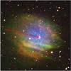 |
Fig. 1 A 35: narrow-band composite of Hα, [O III], and [S II] (in total 36 h exposure time) by Dean Salman (Sh 2 − 313, http://www.sharplesscatalog.com/). N is up, E is left, the FOV is 20′ × 20′. The (red) arrow indicates the projected motion of BD−22°3467 during the last 10 000 years. |
Borkowski et al. (1990) explained the PN asymmetry (Fig. 1) as the result of an interaction between the PN and the surrounding interstellar medium (ISM), the observed bow shock (the star is moving with v = 125 km s-1) being located at the equilibrium sphere of ram pressure of the accelerated PN gas and the stellar wind ram pressure.
A mean (Hipparcos, Tycho-2, and UCAC-2 values) proper motion of μα = −60.95 ± 1.5 mas/yr and μδ = −14.63 ± 1.4 mas/yr was measured by Kerber et al. (2008) in agreement with Hipparcos values (HIP 62905, Van Leeuwen 2007) of μα = −60.91 ± 1.62 mas/yr μδ = −13.41 ± 1.24 mas/yr. With its high proper motion, BD−22°3467 passes through the complete visible nebula within about 16 000 years (Fig. 1). Recently, Frew & Parker (2010) claimed A 35 to be a “bow shock nebula in a photoionized Strömgren sphere in the ambient ISM”. This scenario does not include a PN. Weidmann & Gamen (2011), however, classified A 35 as a binary PN (? + G8 IV) with a bc-CSPN (corresponding to binarity for the cool CSPN).
Hipparcos measured a parallax of 7.48 ± 1.55 mas (Perryman et al. 1997,  ). This was corrected later by Gatti et al. (1998) to
  (this value was adopted by Herald & Bianchi 2002). Gatti et al. (1998) determined a separation of the hot and cool component of 13−28 AU at this distance. However, they adopted 160 pc as a minimum distance because previous estimates (see their Table 2) gave much higher values (e.g. 360 ± 80 pc from photometry measured by Jacoby 1981). Van Leeuwen (2007) presented a validation of the new Hipparcos reduction. The improved parallax (8.38 ± 1.57 mas) is slightly larger with a similar error range. The corresponding distance of
  is now even smaller.
Herald & Bianchi (2002) determined the atmospheric parameters of both components and found Teff = 80 kK, log g = 7.7 (cm/s2) for the WD, and Teff = 5 kK, log g = 3.5 for its companion star. Their hot-component analysis of ultraviolet (UV) spectra (FUSE2, HST/STIS3, and IUE4) covering 905 Å ≲ λ ≲ 3280 Å was performed with TLUSTY and SYNSPEC (Hubeny 1988; Hubeny & Lanz 1992, 1995; Hubeny et al. 1994). They determined abundances for He, C, N, O, Si, and Fe (Table 4). For the analysis of the cool companion they used local thermodynamic equilibrium (LTE) models (Kurucz 1991).
State-of-the-art non-local thermodynamic equilibrium (NLTE) model atmospheres are fully metal-line blanketed and can consider all elements from hydrogen to nickel (Rauch 2003; Rauch et al. 2007). Therefore, we decided to re-analyze the available UV spectra of BD−22°3467 to determine abundances of hitherto neglected metals. The resulting abundance pattern can give clues to the evolutionary history of the DAO star. We begin with a brief description of the observed UV spectra and preparatory work (Sect. 2), followed by an introduction to our model atmospheres (Sect. 3). Then we describe our spectral analysis (Sect. 4) in detail and discuss the results in Sect. 5.
2. Observations and interstellar absorption
Hot post-AGB (asymptotic giant branch) stars have their flux maximum in the UV wavelength range. Most of the exhibited metal lines are located there. Metal lines of successive ionization stages allow one to evaluate the ionization equilibrium of the respective species. This is a very sensitive indicator for Teff. The error ranges of Teff and abundance determinations can be reduced by the analysis of many spectral lines.
The dominant ionization stages of the iron-group elements in the relevant Teff and log g regime are v and vi (Fig. 2). Many strategic lines of these ions are located in the UV wavelength range. We therefore retrieved FUSE, HST/STIS, and IUE observations from the MAST5 archive (Table 1).
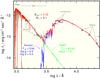 |
Fig. 3 UV-optical-IR flux distribution of the BD−22°3467 binary system, fitted by atmosphere models for both components. |
Our spectral analysis is based on the high-resolution FUSE and STIS observations. The four STIS spectra were co-added to improve the S/N. Herald & Bianchi (2002) analyzed the same FUSE spectrum but only one (O4GT02010) of the STIS spectra. The low-resolution IUE6 observations were used in addition to determine the interstellar reddening (EB − V, Fig. 3) as well as to verify the flux calibration. The STIS observation had to be scaled by a factor of 1.995 to match the flux level of the IUE observation. This offset is possibly due to bad centering of the exciting star during the exposure (Herald & Bianchi 2002).
2.1. Interstellar absorption and reddening
The general procedure of determining the interstellar reddening is to normalize a theoretical spectrum as far as possible in the low-energy range because it is not significant there. In the case of BD−22°3467, the companion star dominates the observation at wavelengths longer than ≈ 2800 Å. Therefore, we constructed a theoretical, composite spectrum (with appropriate stellar radii,  ) using our final model spectrum (Teff = 80 kK, log g = 7.2) and a Kurucz model7 (Teff = 5000 K, log g = 3.5, solar abundances log Z = 0.0) for the hot and cool component, respectively. This spectrum was then normalized to the 2MASS K flux (Fig. 3). The best fit (matching all GALEX, Hipparcos, and 2MASS magnitudes and the UV spectra) was achieved for EB − V = 0.02 ± 0.02, using the reddening law of Fitzpatrick (1999) with the standard Rv = 3.1. Our value agrees within error limits with those of Herald & Bianchi (2002, EB − V = 0.04 ± 0.01, who used the Rayleigh-Jeans tail of the UV observations (1000 Å ≲ λ ≲ 2800 Å) only.
To determine the column density of interstellar neutral hydrogen, nH I, models with different nH I were compared with Ly α. We found a best fit for nH I = 5.0 ± 1.5 × 1020 cm-2 (Fig. 4), which agrees with the value found by Herald & Bianchi (2002).
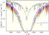 |
Fig. 4 STIS observation around H I Ly α compared with our final model (Table 4) at different nH I. The dashed line is the WD’s atmospheric flux. |
2.2. Radial velocity of the hot component
The STIS observation shows numerous sharp, isolated photospheric lines that are suitable to determine vrad. On average (21 lines of N V, O IV, O V, Ar V, Cr V, Cr VI, Fe V, Fe VI, and Ni V), we measured vrad = −14.4 ± 0.7 km s-1.
3. Model atmospheres and atomic data
In this section, we briefly describe the atomic data and the programs used for our analysis. Details about the calculation of the stellar atmosphere models can be found in Sect. 3.1. The usage of OWENS for the calculation of the ISM absorption is described in Sect. 3.2.
3.1. The photospheric model for the hot component
Our model atmospheres (plane-parallel, chemically homogeneous, in hydrostatic and radiative equilibrium) are calculated with TMAP8, the Tübingen NLTE model atmosphere package (Werner et al. 2003). We calculated a small grid of models that include opacities of 23 elements from H–Ni (Table 2).
H–Ar are represented by “classical” model atoms (Rauch 1997) taken from TMAD9, the Tübingen model atom database. For Ca–Ni, a statistical approach was applied to handle the large number of atomic levels and line transitions. We employed IrOnIc (Rauch & Deetjen 2003; Rauch 2003) to consider thousands of levels and millions of lines provided by Kurucz (2009, and priv. comm.) and the Opacity Project (Seaton et al. 1994).
Kurucz‘s line lists are divided into so-called LIN (measured and theoretical lines) and POS (only measured, “good” wavelengths) lists. For the model-atmosphere calculations, the LIN lists were used, to consider the total opacity properly. To calculate the emerging spectrum, POS lists were used to identify iron-group lines. Figure 5 demonstrates the difference between LIN and POS line lists. As an example for all species and their ions serves Cr V (within the shown 1470 − 1500 Å interval). At present, Kurucz provides 73 222 LIN and 249 POS lines of Cr V, 459 LIN and 6 POS lines in this wavelength interval. We adjusted the Cr abundance to [Cr] = + 3.1 to reproduce the two strongest Cr V POS lines, Cr V λλ 1482.76,1489.71 Å. At this abundance, most of the prominent Cr V LIN lines appear displaced or simply too strong. An exception is Cr V λ 1481.66 Å, which matches the observation well. It can not be excluded that the Cr V λ 1490.24 Å LIN lines in the model is the observed 1490.66 Å line, for instance. However, reliable abundance determinations are only possible using unambiguously identified POS lines (Sect. 4.3).
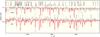 |
Fig. 5 Section of the STIS spectrum (black line) compared with our TMAP model. The SED in the upper panel was calculated using Kurucz’s POS data (the strongest lines are identified at top), the SED in the lower panel using LIN data. This section contains mainly Fe v–vi and Mn v–vi lines. The strongest Cr V LIN lines are identified at the bottom. |
In the framework of the Virtual Observatory (VO10), all spectral energy distributions (SEDs, λ − Fλ) calculated from our model-atmosphere grid are available in VO-compliant form from the registered VO service TheoSSA11 provided by the German Astrophysical Virtual Observatory (GAVO12).
3.2. The ISM line-absorption model
In the FUSE wavelength range (Fig. 6), numerous interstellar H2 and H I absorption lines hamper the analysis of the photospheric spectrum. We applied the program OWENS to calculate ISM line-absorption models. OWENS allows one to model different clouds with distinct radial and turbulent velocities, temperatures, column densities, and chemical compositions. It fits Voigt profiles using a χ2 minimization. For more information on OWENS, see e.g. Hébrard et al. (2002) or Hébrard & Moos (2003).
Figure 6 shows a small section of the FUSE spectrum of BD−22°3467. Only the combination of the photospheric and ISM-model spectra reproduces most of its spectral features. Our ISM model includes lines of H I, H2 (J = 0−9), HD, C II − IV, N I– III, N V, O I, O VI, Mg II, Al II, Si II– IV, P II, S II– III, S VI, Ar I− II, Mn II, Fe II, and Ni II. The radial velocity of the interstellar low-ionization (i–ii) atomic gas and H2 is found to be vrad = 6 ± 2 km s-1.
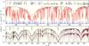 |
Fig. 6 Top: section of the FUSE observation showing the necessity of a detailed modeling of the ISM. The dashed line is the final, pure photospheric model. The full (red) line shows a combined stellar and interstellar model. Blue marks at the bottom denote interstellar H2 absorption lines. Bottom: comparison of (pure photospheric) TMAP models with log g = 7.2 (thick, black) and log g = 7.7 (thin, red), normalized to the flux of the log g = 7.2 model at 999 Å for comparison. The full lines are calculated with the determined reddening of |


4. Analysis
In this section, we begin with a verification of those atmospheric parameters that were already determined by Herald & Bianchi (2002) which may deviate because these authors used TLUSTY and considered He, C, N, O, Si, and Fe, while we employed TMAP with far more elements (Table 2). This might result in a different atmospheric structure. We begin with models with parameters of Herald & Bianchi (2002) and fine-tune them if necessary.
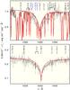 |
Fig. 7 Spectra of our final model compared with the FUSE and STIS observations around He II λ 1084.94 Å (top, dashed: pure photospheric, full line: photospheric + ISM line absorption) and He II λ 1640.42 Å (bottom, dashed: log g = 7.7, full line: log g = 7.2). The identified lines are marked. Most of the very strong absorptions in the top panel stem from H2. |
4.1. Effective temperature and surface gravity
Herald & Bianchi (2002) determined Teff = 80 kK and log g = 7.7. TMAP test calculations showed that their Teff value matches all ionization equilibria well, e.g. N IV/N V, O IV/O V, and Mn V/Mn VI (Sect. 4.3). A lower log g = 7.2 yields a significantly better fit agree of the theoretical He II λ 1640.42 Å line profile with the observation in the line core, which is not matched at log g = 7.7 (Fig. 7). For the line-profile calculations, we used the Stark line-broadening tables by Schöning & Butler (1989a,b). The line wings are too broad at log g = 7.7 and somewhat too weak at log g = 7.2. The same is true for He II λ 1084.94 Å (Fig. 7). The decrements of spectral line series such as the H I Balmer (Rauch et al. 1998), H I Lyman (transitions n − n′ = 1–3 to 1–8), and He II 2–n′ series (2 − 5 to 2 − 11) are strongly dependent on log g. The fit to the outer line wings of the latter two series in the FUSE spectrum is also very well reproduced at log g = 7.2. Figure 6 shows He II 2–5 to 2–14 and the respective H I 1–3 to 1–7 blends. A comparison of their theoretical profiles at log g = 7.2 and log g = 7.7 with the observation shows that they are significantly too broad at log g = 7.7. This effect cannot be compensated for by a lower EB − V (Fig. 6). The interstellar H I absorption is not dominating the wings of these lines. The observed “shoulders” between the H I Lyman lines and, thus, the Lyman decrement is well reproduced at log g = 7.2 and is definitely missed at log g = 7.7. This is best visble between Ly ζ and Ly δ because the contamination of the FUSE observation with ISM lines is obviously weak. log g = 7.2 agrees with the value of Herald & Bianchi (2002) within realistic error limits of 0.3 dex. Their assumed statistical error ( ) seems to be too optimistic. We finally adopted Teff = 80 ± 10 kK and log g = 7.2 ± 0.3 for our analysis.
4.2. Hydrogen and helium
We adopted [He] = −0.3 ( [X] denotes log [mass fraction/solar mass fraction] for species X) from Herald & Bianchi (2002) and achieved a reasonable fit to the He II lines (Fig. 7).
4.3. Metal abundances
In our TMAP model-atmosphere calculations, we considered opacities of all elements from H to Ni except for Li, Be, B, Cl, and K. We convolved our synthetic spectra with Gaussians to simulate the respective instrument resolution. By comparison with the observed spectrum of BD−22°3467, we determined for the first time photospheric abundances of Ar, Cr, Mn, Co, and Ni. All identified lines of these species in the available observations (Sect. 2) were evaluated in our abundance analysis. No lines of F, Ne, Na, Mg, Al, Ca, Sc, Ti, and V were identified. For these, only upper limits could be derived by test models where the respective lines in the model emerge (at the abundance limit) from the noise in the observation. A detailed comparison of models with different abundances of individual metals showed that the typical abundance error is ± 0.3 dex. In the following, we briefly describe some measurements (ordered by increasing atomic weight).
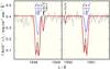 |
Fig. 8 C IV λλ 1548.20,1550.77 Å lines in the STIS observation compared with our final model. Blue, thin: photospheric lines, red, thick: photospheric + interstellar lines, black, thin: interstellar lines. |
Carbon:
lines of stellar origin are not detectable in the spectrum of BD−22°3467. Narrow interstellar C IV λλ 1548.20,1550.77 Å lines are present (Fig. 8) that virtually “bracket” the photospheric lines ( km s-1, Sect. 2.2). They have their origin in two different interstellar “clouds” with different radial velocities and column densities (cloud 1: vrad = −5.4 km s-1, log (nC IV/(g/cm2)) = 16.8; cloud 2: vrad = −30.4 km s-1, log (nC IV/(g/cm2)) = 14.6). The radial velocity of cloud 1 agrees with the velocity of the low-ionization ISM gas (Sect. 3.2). Interestingly, Schneider et al. (1983) determined vrad = −6.6 ± 3.8 km s-1 for the nebula. This even suggests a nebular origin of cloud 1 while cloud 2 with its significantly higher velocity lies on the line of sight toward us.
It is worthwhile to note that no other interstellar two-component absorption-line feature is identified in the spectrum of BD−22°3467.
However, a photospheric component, even at low abundance, worsens the agreement between model and observation in the shoulder between the interstellar lines (Fig. 8). Since the strongest C IV lines in the FUSE wavelength range (λλ948,1107,1168 Å) become too strong for [C] > −2.9, we determine this as an upper limit. This value is about four times lower than that found by Herald & Bianchi (2002).
Nitrogen:
N IV λ 1718.55 Å and N V λλ 1238.82,1242.80 Å are prominent in the STIS observation. Our final model reproduces the strengths of these lines and the ionization equilibrium at [N] = −1.7 (Fig. 9) well.
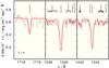 |
Fig. 9 N IV λ 1718.55 Å and N V λλ 1238.82,1242.80 Å lines in the STIS observation compared with our final model. |
Herald & Bianchi (2002) determined a much lower photospheric N abundance (<10-3 times the solar value) because of strong line wings forming at higher abundances. The reason may be a different approximation by the quadratic Stark effect in TMAP and TLUSTY/SYNSPEC.
For the line-absorption cross-sections TMAP calculates 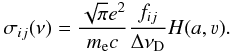 (1)e and me are electron charge and mass, c is the light velocity, ΔνD the Doppler width, fij the oscillator strength for the transition i → j, and H the Voigt function with
 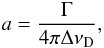 (2)and
  (3)where Δν = ν − ν0 with the line frequency ν0.
According to Cowley (1970, 1971), the line-broadening due to the quadratic Stark effect is approximately given by ![Mathematical equation: \begin{equation} \Gamma_{\rm Stark} = 5.5\times10^{-5}\;\frac{n_{\rm e}}{\sqrt{T}}\;\left [\,\frac{(n_\mathrm{eff}^\mathrm{up})^2}{z+1}\,\right]^2 , \end{equation}](/articles/aa/full_html/2012/12/aa19536-12/aa19536-12-eq103.png) (4)where ne is the electron density, T is the temperature,
(4)where ne is the electron density, T is the temperature,  is the effective principal quantum number of the upper level, and z is the effective charge seen by the active electron. Radiative (Γrad) and collisional damping by electrons is considered so that
 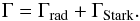 (5)TMAP uses fij of 7.8580 × 10⁻² and 1.5716 × 10⁻¹, and classical damping constants Γrad of 1.4401 × 10 + 9 and 1.4494 × 10 + 9 for N V Å, respectively.
A comparison of calculated ΓSt values (Sahal-Bréchot, priv. comm.) has shown that 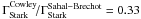 is a good approximation for the N V resonance doublet within 10 000 < T/K < 200 000. We introduced this factor and adopted
  for our analysis.
Oxygen:
is present in the spectra with the ionization stages iv and v. We can reproduce the ionization equilibrium and the line strengths. Figure 10 shows O IV λλ 1338.61,1343.51 Å and O V λ 1371.29 Å at [O] = −2.6. This agrees well with the observation and the value of Herald & Bianchi (2002).
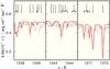 |
Fig. 10 O IV λλ 1338.61,1343.51 Å (left and middle) and O V λ 1371.29 Å (right) lines in the STIS observation compared with our final model. |
Fluorine:
was not identified in the observation. We modeled F V λλ 1082.31,1088.38 Å and F VI λ 1139.49 Å. They would be visible in the observation at abundances higher than solar.
Magnesium:
lines are weak and almost fade in the noise, even the strongest, Mg IV λ 1683.003 Å. Figure 5 shows Mg IV λ 1490.433 Å, which is not detectable in the FUSE observation at solar abundance. Thus, we can only determine an upper abundance limit of [Mg] = 0.0.
Silicon:
exhibits only the Si IV λλ 1393.76,1402.77 Å resonance doublet (Fig. 11), other Si lines are too weak. A weak ISM contamination is present but we can determine [Si] = −2.1. This agrees well with the upper limit of Herald & Bianchi (2002).
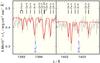 |
Fig. 11 Si IV λλ 1393.76,1402.77 Å in the STIS observation compared with our final model. |
Argon:
is strongly enhanced ( [Ar] = + 1.1). Similar to the central star of the PN Sh 2–216, LS V + 46°21 (cf. Rauch et al. 2007), Ar VI Å are identified in the STIS observation (Fig. 12) and reproduced by our final model. Our models show a strong Ar VII λ 1063.55 Å line but this is blended by interstellar H2 absorption and therefore not suitable for a Teff determination via the ionization equilibrium.
A problem are lines like Ar V λ 1371.92 Å (Fig. 10) which are much stronger in our models than observed. Since many ionization equilibria of different species such as Mn v − vi (see below) are well-matched, a higher Teff that would shift the ionization balance from Ar V to Ar VI can be excluded. We checked the possibility that the oscillator strengths of Ar V lines that we use in TMAP (from the Opacity Project, Seaton et al. 1994) are too strong. The Ar V triplet 3p3 3S°–3p4 3P (Ar V Å) is found in Opacity Project data (far off) at 1455.77 Å (without fine-structure splitting) with f = 4.2333 × 10⁻². From this value, we calculated f-values of 4.7037 × 10⁻², 1.4111 × 10⁻², and 2.3518 × 10⁻² for the three fine-structure components. A comparison with recent work of Tayal et al. (2009, f1371.92 = 2.257 × 10⁻² and 2.834 × 10⁻² shows good agreement with the Opacity Project. Thus, the reason for the disagreement of the Ar V lines remains unknown.
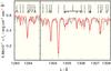 |
Fig. 12 Section of the STIS spectrum around Ar vi λλ 1283.96, 1303.89, 1307.38 Å compared with our final, composite photospheric and ISM spectrum. |
Chromium:
is about 70 times enhanced ( [Cr] = +1.8). In Fig. 14), Cr VI λλ 1417.66,1455.28 Å are shown that are well-reproduced by our final model. Cr V λλ 1482.76,1489.71 Å (Fig. 5) would require a much higher [Cr] = +3.1 (Sect. 3.1). Since Teff and log g are well-determined (Sect. 4.1) and, thus, a strong change of the ionization balance toward Cr V is impossible within the error limits, we have to consider these two lines as blends and not suited for a reliable abundance determination.
Manganese:
exhibits several Mn V and VI lines in the STIS wavelength range, e.g. (the strongest) Mn V λλ 1359.24, 1382.88, 1432.84, 1440.31, 1443.31, 1452.88, 1457.46, 1480.75, 1486.50 Å and Mn VI λλ 1272.44, 1285.10, 1333.87, 1345.49, 1356.85, 1391.17, 1391.22, 1548.43 Å (Fig. 13). All these lines are reproduced at [Mn] = +1.5. Since many lines of two successive ionization stages are suitable for spectral analysis, the Mn v–vi ionization equilibrium is one of the prime indicators for Teff for BD−22°3467. Teff = 80 kK is well-matched at log g = 7.2 (Sect. 4.1).
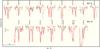 |
Fig. 13 Strongest Mn V (top) and Mn VI lines (bottom) in the STIS wavelength range compared with our final model. |
Mass, luminosity, radius, distance, and height above the Galactic plane of BD−22°3467.
Iron:
has many lines of Fe V and VI in the UV spectrum. In contrast to Herald & Bianchi (2002), who determined a 0.1 − 0.5 times solar Fe abundance, we find it approximately solar (e.g. Fig. 5). There are, however, some Fe lines that are stronger in our model than observed (see some Fe VI lines in Fig. 14, bottom panel). Within the error range, we find the same Fe abundance as Herald & Bianchi (2002).
Cobalt:
is strongly enhanced. Co V λλ 1331.50,1349.60 Å indicate [Co] = +2.2 (Fig. 14).
Nickel:
is also overabundant. Numerous Ni V and VI lines are found in the UV spectrum. They are all reproduced at [Ni] = +0.7 (e.g. Figs. 5, 14).
4.4. Mass, luminosity, radius, and distance
We determined the stellar mass and luminosity from a comparison with evolutionary tracks for hydrogen-rich post-AGB stars (Fig. 15, Miller Bertolami, priv. comm.) and for post-EHB (extended horizontal branch) stars from Dorman et al. (1993, Fig. 17. The results are summarized in Table 3.
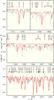 |
Fig. 14 Sections of the STIS observation containing (in addition to others) lines of Cr VI (top), Co (middle), and Ni (bottom) compared with our final model. |
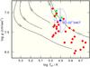 |
Fig. 15 Location of BD−22°3467 in the log Teff – log g diagram compared with other DAO-type WDs taken from Gianninas et al. (2010, all symbols). Three of these (green squares) are used to compare their metal abundances with those of BD−22°3467 (Fig. 16). The post-AGB evolutionary tracks were calculated by Miller Bertolami (priv. comm.) labeled with the stellar mass (in M⊙). |
The stellar radius follows from  , where G is the gravitational constant. We determined the spectroscopic distance
  (Table 3) following Wassermann et al. (2010). It is derived from
  (6)with the astrophysical flux Fν at the surface of the star as predicted by the model spectrum, and Fobs is the observed, extinction-corrected flux (we used F1513 Å to match the center of the GALEX far-ultraviolet band). D is about three times larger than the improved Hipparcos distance (
 , Sect. 1) but it agrees with the photometric distance (360 ± 80 pc, Jacoby 1981) for the cool component.
It is worthwhile to mention that there is no agreement with the Hipparcos distance at the maximum value of log g = 7.83 given by Herald & Bianchi (2002) either. The calculated spectroscopic distance (using M = 0.68 M⊙, R = 0.017 R⊙, and the respective model flux) is then D = 226 pc, about twice the Hipparcos distance. Although trigonometric parallaxes in general have to be regarded as hard constraints, orbital movement in binary systems such as BD−22°3467 may bear on the precision of Hipparcos measurements (cf. Rauch 2000, for LB 3459 = TYC 9166−00716−1). Figures 6 and 7 clearly demonstrate that the spectra cannot be reproduced with a gravity of log g = 7.7 or higher, while a good fit is achieved for log g = 7.2. The upcoming GAIA mission will provide a highly precise parallax for BD−22°3467 which will be able to rule out the uncertainties.
5. Results and discussion
We calculated a grid of TMAP NLTE models atmospheres for BD−22°3467, the exciting star of the ionized nebula A 35. We determined Teff = 80 ± 10 kK and log g = 7.2 ± 0.3, and thus confirm Teff = 80 kK found by Herald & Bianchi (2002). Nevertheless, we found a somewhat lower log g than Herald & Bianchi (2002, log g = 7.7. For the first time in this object, abundances from detailed line-profile fits were determined for Ar, Cr, Mn, Co, and Ni (Table 4). For F, Ne, Na, Mg, Al, Ca, Sc, Ti, and V, upper limits could be derived.
Results of this work compared with Herald & Bianchi (2002), whose He abundance we adopted.
The element abundance pattern (Fig. 16) is probably the result of the interplay of radiative levitation and gravitational settling. Compared to those objects in the DAO sample from Good et al. (2004, 2005) that have the same Teff and log g within error limits, BD−22°3467 has a higher He and a lower Si abundance. Cr, Mn, Co, and Ni (not measured by Good et al. 2005) are strongly overabundant, likely due to the force of the radiation field. Radiative levitation may be a reason but the question remains why Fe is about solar. Detailed diffusion calculations that consider these elements are highly desirable investigating this phenomenon. A comparison with existing diffusion calculations (Chayer et al. 1995a,b, Fig. 16) shows (within error limits) that the metal abundances partially agree with predictions for DA-type WDs. Only N, Mg, S, and Ca are more than one dex lower than predicted.
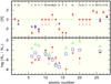 |
Fig. 16 Top: photospheric abundances of BD−22°3467 compared with solar values (Asplund et al. 2009), and mean values from three objects of Good et al. (2005, blue triangles) that are located within the error ellipse (cf. Fig. 15, green squares there). Arrows indicate upper limits. Bottom: comparison of number ratios compared with predictions of diffusion calculations for hydrogen-rich (DA-, blue squares) and helium-rich (DO-type, green triangles) WDs (Chayer et al. 1995a,b) with Teff = 80 kK and log g = 7.2. |
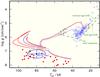 |
Fig. 17 Location of BD−22°3467 in the Teff – log g diagram compared with sd(O)B-type stars close to the EHB taken from Edelmann (blue, open squares 2003) and DAO-type WDs taken from Gianninas et al. (red diamonds and green, filled squares 2010, cf. Fig. 15. The post-EHB evolutionary tracks are from Dorman et al. (1993, Y = 0.288 ≈ Y⊙ and labeled with the stellar mass (in M⊙). |
Until recently, BD−22°3467 was believed to be the central star of a planetary nebula and, thus, a post-AGB evolution of an intermediate-mass star (0.8 M⊙ ≲ Minitial ≲ 8.0 M⊙) appeared to be a matter of course. Frew & Parker (2010) showed that the visible, PN-like nebula may be a combination of shock excitation and photoionization of the ambient interstellar gas.
BD−22°3467 provides enough high-energy photons, (4.4 × 1025 photons/s/cm2 at energies > 13.6 eV and 6.4 × 10²² photons/s/cm2 at energies > 54 eV calculated from our final model which give totals of N13 = 2.3 × 1045 photons/s and N54 = 3.3 × 1042 photons/s, respectively) to ionize the surrounding interstellar gas (cf. Rauch et al. 2004). For N54/N13 < 0.01, no He II emission from the nebula can be expected. If we assume an electron temperature of Te = 10 000 K in the nebula, negligible extinction, d = 361 pc (Table 4), and an average angular diameter of 750 ′′, we derive that BD−22°3467 has a Strömgren sphere with a density of 16 cm-3, log (FH β/erg/s/cm2) = −11.23, and an ionized nebular mass of 0.5 M⊙. The absolute H β flux agrees very well with the value given by Acker et al. (1992, log FH β = −11.3.
The nebular spectrum by Acker & Stenholm obtained for the catalog (Acker et al. 1992) is weak and, consequently, the FH α/FH β ratio is overestimated, and the derived extinction of c = 0.7 is very uncertain. F [O III] λ5007 Å/FH β = 2 indicates low excitation. Both N II λλ 6548,6584 Å are visible and, with standard assumptions for the nebula but without any correction for unseen higher ionization stages of nitrogen, its nebular abundance may be estimated to be 12 + log N/H = 7.7. The Si II λ 6716 Å/Si II λ 6731 Å line intensity ratio is at the low-density limit and we can conclude that the nebular electron density is ne < 100 cm3. In addition, we may estimate that the nebular oxygen and sulfur abundances are 7.9 and 6.4, respectively. It is worthwhile to note that the ionized mass of 0.5 M⊙ is of about the value usually assumed for the average PN mass of 0.2−0.3 M⊙. The reason is simply the fairly low luminosity of BD−22°3467. Such a low-luminosity ionizing star makes a Strömgren sphere that may well mimic a genuine PN. It is thus possible that similar objects have been misclassified as PNe.
Because the time since its departure from the AGB is relatively long for BD−22°3467 due to its low mass (Table 3), all matter ejected previously on the AGB (as well as the PN) may have dissipated into the ambient ISM. Thus, the result of Frew & Parker (2010) does not stringently exclude a post-AGB evolution. However, an alternative stellar evolution may be possible. Bergeron et al. (1994) discussed that the progenitors of most DAO-type WDs are post-EHB stars (M ≈ 0.48 M⊙). Recently, Gianninas et al. (2010) presented a spectral analysis of 29 DAO- and 18 hot DA-type WDs and found that their DAOs (Fig. 15) are hotter and more massive that previously determined. Accordingly, they concluded that most of these (“a rather mixed bag of objects”) are products of post-AGB evolution. BD−22°3467 is located amongst the low-mass stars of their sample (Fig. 17) and consequently, a post-EHB evolution cannot be ruled out. In this scenario, the stars evolve directly from the EHB to the WD state (AGB-manqué stars, Greggio & Renzini 1990). Bergeron et al. (1994) proposed that a weak mass-loss may keep enough helium in the line-forming regions (Unglaub & Bues 1998, 2000) to exhibit strong He II absorption lines. Figure 17 shows BD−22°3467 in comparison to post-EHB evolutionary tracks (Dorman et al. 1993). One can estimate that an M ≈ 0.48 M⊙ track (with solar helium content on the horizontal branch, HB) will match the position of BD−22°3467. (Dorman’s tracks for masses higher than 0.475 M⊙ and solar helium content are not fully calculated down to lower Teff and higher log g.) On its way from the EHB to its present position, i.e., towards higher Teff and higher log g, gravitational settling, radiative levitation, and a weak wind are interacting and, thus, the atmospheric abundances may deviate from the HB abundances.
Online material
Log of the UV observations of BD−22°3467.
Statistics of H – Ar model atoms used in our calculations.
Continued for Ca–Ni.
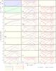 |
Fig. 2 Temperature and electron density stratification along with ionization fractions of all elements in our final model. |
Spectral classification: characteristic H I and He II absorption lines.
Far Ultraviolet Spectroscopic Explorer.
Hubble Space Telescope/Space Telescope Imaging Spectrograph.
International Ultraviolet Explorer.
International Ultraviolet Explorer.
ftp://ftp.stsci.edu/cdbs/grid/k93models/kp00/
Acknowledgments
M.Z. was supported by the German Research Foundation (DFG, grant WE1312/38-1). T.R. is supported by the German Aerospace Center (DLR, grant 05 OR 0806). This research has made use of the SIMBAD database, operated at CDS, Strasbourg, France. This research has made use of NASA’s Astrophysics Data System. This work used the profile-fitting procedure OWENS developed by M. Lemoine and the FUSE French Team. Some of the data presented in this paper were obtained from the Mikulski Archive for Space Telescopes (MAST). STScI is operated by the Association of Universities for Research in Astronomy, Inc., under NASA contract NAS5-26555. Support for MAST for non-HST data is provided by the NASA Office of Space Science via grant NNX09AF08G and by other grants and contracts.
References
- Abell, G. O. 1955, PASP, 67, 258 [NASA ADS] [CrossRef] [Google Scholar]
- Abell, G. O. 1966, ApJ, 144, 259 [NASA ADS] [CrossRef] [Google Scholar]
- Acker, A., Marcout, J., Ochsenbein, F., et al. 1992, The Strasbourg-ESO Catalogue of Galactic Planetary Nebulae, Parts I, II [Google Scholar]
- Asplund, M., Grevesse, N., Sauval, A. J., & Scott, P. 2009, ARA&A, 47, 481 [NASA ADS] [CrossRef] [Google Scholar]
- Bergeron, P., Wesemael, F., Beauchamp, A., et al. 1994, ApJ, 432, 305 [NASA ADS] [CrossRef] [Google Scholar]
- Borkowski, K. J., Sarazin, C. L., & Soker, N. 1990, ApJ, 360, 173 [NASA ADS] [CrossRef] [Google Scholar]
- Chayer, P., Vennes, S., Pradhan, A. K., et al. 1995a, ApJ, 454, 429 [NASA ADS] [CrossRef] [Google Scholar]
- Chayer, P., Fontaine, G., & Wesemael, F. 1995b, ApJS, 99, 189 [NASA ADS] [CrossRef] [Google Scholar]
- Cowley, C. R. 1970, The theory of stellar spectra (New York: Gordon & Breach) [Google Scholar]
- Cowley, C. R. 1971, The Observatory, 91, 139 [NASA ADS] [Google Scholar]
- De Marco, O. 2009, PASP, 121, 316 [NASA ADS] [CrossRef] [Google Scholar]
- Dorman, B., Rood, R. T., & O’Connell, R. W. 1993, ApJ, 419, 596 [CrossRef] [Google Scholar]
- Edelmann, H. 2003, Dissertation, University of Erlangen-Nuremberg [Google Scholar]
- Fitzpatrick, E. L. 1999, PASP, 111, 63 [NASA ADS] [CrossRef] [Google Scholar]
- Frew, D. J., & Parker, Q. A. 2010, PASA, 27, 129 [NASA ADS] [CrossRef] [Google Scholar]
- Gatti, A. A., Drew, J. E., Oudmaijer, R. D., Marsh, T. R., & Lynas-Gray, A. E. 1998, MNRAS, 301, L33 [NASA ADS] [CrossRef] [Google Scholar]
- Gianninas, A., Bergeron, P., Dupuis, J., & Ruiz, M. T. 2010, ApJ, 720, 581 [NASA ADS] [CrossRef] [Google Scholar]
- Good, S. A., Barstow, M. A., Holberg, J. B., et al. 2004, MNRAS, 355, 1031 [NASA ADS] [CrossRef] [Google Scholar]
- Good, S. A., Barstow, M. A., Burleigh, M. R., et al. 2005, MNRAS, 363, 183 [NASA ADS] [CrossRef] [Google Scholar]
- Greggio, L., & Renzini, A. 1990, ApJ, 364, 35 [Google Scholar]
- Grewing, M., & Bianchi, L. 1988, in ESA Spec. Publ., 281, 177 [Google Scholar]
- Hébrard, G., & Moos, H. W. 2003, ApJ, 599, 297 [NASA ADS] [CrossRef] [Google Scholar]
- Hébrard, G., Friedman, S. D., Kruk, J. W., et al. 2002, Planet. Space Sci., 50, 1169 [NASA ADS] [CrossRef] [Google Scholar]
- Herald, J. E., & Bianchi, L. 2002, ApJ, 580, 434 [NASA ADS] [CrossRef] [Google Scholar]
- Hubeny, I. 1988, Comp. Phys. Comm., 52, 103 [Google Scholar]
- Hubeny, I., & Lanz, T. 1992, A&A, 262, 501 [NASA ADS] [Google Scholar]
- Hubeny, I., & Lanz, T. 1995, ApJ, 439, 875 [Google Scholar]
- Hubeny, I., Hummer, D. G., & Lanz, T. 1994, A&A, 282, 151 [NASA ADS] [Google Scholar]
- Jacoby, G. H. 1981, ApJ, 244, 903 [NASA ADS] [CrossRef] [Google Scholar]
- Kerber, F., Mignani, R. P., Smart, R. L., & Wicenec, A. 2008, A&A, 479, 155 [NASA ADS] [CrossRef] [EDP Sciences] [Google Scholar]
- Kurucz, R. L. 1991, in Stellar Atmospheres – Beyond Classical Models, eds. L. Crivellari, I. Hubeny, & D. G. Hummer, NATO ASIC Proc., 341, 441 [Google Scholar]
- Kurucz, R. L. 2009, in AIP Conf. Ser. 1171, eds. I. Hubeny, J. M. Stone, K. MacGregor, & K. Werner, 43 [Google Scholar]
- Perryman, M. A. C., Lindegren, L., Kovalevsky, J., et al. 1997, A&A, 323, L49 [NASA ADS] [Google Scholar]
- Rauch, T. 1997, A&A, 320, 237 [NASA ADS] [Google Scholar]
- Rauch, T. 2000, A&A, 356, 665 [NASA ADS] [Google Scholar]
- Rauch, T. 2003, A&A, 403, 709 [NASA ADS] [CrossRef] [EDP Sciences] [Google Scholar]
- Rauch, T., & Deetjen, J. L. 2003, in Stellar Atmosphere Modeling, eds. I. Hubeny, D. Mihalas, & K. Werner, ASP Conf. Ser., 288, 103 [Google Scholar]
- Rauch, T., Dreizler, S., & Wolff, B. 1998, A&A, 338, 651 [NASA ADS] [Google Scholar]
- Rauch, T., Kerber, F., & Pauli, E.-M. 2004, A&A, 417, 647 [NASA ADS] [CrossRef] [EDP Sciences] [Google Scholar]
- Rauch, T., Ziegler, M., Werner, K., et al. 2007, A&A, 470, 317 [NASA ADS] [CrossRef] [EDP Sciences] [Google Scholar]
- Schneider, S. E., Terzian, Y., Purgathofer, A., & Perinotto, M. 1983, ApJS, 52, 399 [NASA ADS] [CrossRef] [Google Scholar]
- Schöning, T., & Butler, K. 1989a, A&AS, 79, 153 [NASA ADS] [Google Scholar]
- Schöning, T., & Butler, K. 1989b, A&AS, 78, 51 [NASA ADS] [Google Scholar]
- Seaton, M. J., Yan, Y., Mihalas, D., & Pradhan, A. K. 1994, MNRAS, 266, 805 [NASA ADS] [CrossRef] [Google Scholar]
- Strassmeier, K. G. 2009, A&ARv, 17, 251 [NASA ADS] [CrossRef] [Google Scholar]
- Tayal, V., Gupta, G. P., & Tripathi, A. N. 2009, Indian J. Phys., 83, 1271 [NASA ADS] [CrossRef] [Google Scholar]
- Unglaub, K., & Bues, I. 1998, A&A, 338, 75 [NASA ADS] [Google Scholar]
- Unglaub, K., & Bues, I. 2000, A&A, 359, 1042 [NASA ADS] [Google Scholar]
- Unruh, Y. C., Gatti, A. A., Drew, J. E., et al. 2001, in 11th Cambridge Workshop on Cool Stars, Stellar Systems and the Sun, eds. R. J. Garcia Lopez, R. Rebolo, & M. R. Zapaterio Osorio, ASP Conf. Ser., 223, 1320 [Google Scholar]
- Van Leeuwen, F. 2007, A&A, 474, 653 [NASA ADS] [CrossRef] [EDP Sciences] [Google Scholar]
- Wassermann, D., Werner, K., Rauch, T., & Kruk, J. W. 2010, A&A, 524, A9 [NASA ADS] [CrossRef] [EDP Sciences] [Google Scholar]
- Weidmann, W. A., & Gamen, R. 2011, A&A, 526, A6 [NASA ADS] [CrossRef] [EDP Sciences] [Google Scholar]
- Werner, K., Deetjen, J. L., Dreizler, S., et al. 2003, in Stellar Atmosphere Modeling, eds. I. Hubeny, D. Mihalas, & K. Werner, ASP Conf. Ser., 288, 31 [Google Scholar]
All Tables
Mass, luminosity, radius, distance, and height above the Galactic plane of BD−22°3467.
Results of this work compared with Herald & Bianchi (2002), whose He abundance we adopted.
All Figures
|
Fig. 1 A 35: narrow-band composite of Hα, [O III], and [S II] (in total 36 h exposure time) by Dean Salman (Sh 2 − 313, http://www.sharplesscatalog.com/). N is up, E is left, the FOV is 20′ × 20′. The (red) arrow indicates the projected motion of BD−22°3467 during the last 10 000 years. |
| In the text | |
|
Fig. 3 UV-optical-IR flux distribution of the BD−22°3467 binary system, fitted by atmosphere models for both components. |
| In the text | |
|
Fig. 4 STIS observation around H I Ly α compared with our final model (Table 4) at different nH I. The dashed line is the WD’s atmospheric flux. |
| In the text | |
|
Fig. 5 Section of the STIS spectrum (black line) compared with our TMAP model. The SED in the upper panel was calculated using Kurucz’s POS data (the strongest lines are identified at top), the SED in the lower panel using LIN data. This section contains mainly Fe v–vi and Mn v–vi lines. The strongest Cr V LIN lines are identified at the bottom. |
| In the text | |
|
Fig. 6 Top: section of the FUSE observation showing the necessity of a detailed modeling of the ISM. The dashed line is the final, pure photospheric model. The full (red) line shows a combined stellar and interstellar model. Blue marks at the bottom denote interstellar H2 absorption lines. Bottom: comparison of (pure photospheric) TMAP models with log g = 7.2 (thick, black) and log g = 7.7 (thin, red), normalized to the flux of the log g = 7.2 model at 999 Å for comparison. The full lines are calculated with the determined reddening of |
| In the text | |
|
Fig. 7 Spectra of our final model compared with the FUSE and STIS observations around He II λ 1084.94 Å (top, dashed: pure photospheric, full line: photospheric + ISM line absorption) and He II λ 1640.42 Å (bottom, dashed: log g = 7.7, full line: log g = 7.2). The identified lines are marked. Most of the very strong absorptions in the top panel stem from H2. |
| In the text | |
|
Fig. 8 C IV λλ 1548.20,1550.77 Å lines in the STIS observation compared with our final model. Blue, thin: photospheric lines, red, thick: photospheric + interstellar lines, black, thin: interstellar lines. |
| In the text | |
|
Fig. 9 N IV λ 1718.55 Å and N V λλ 1238.82,1242.80 Å lines in the STIS observation compared with our final model. |
| In the text | |
|
Fig. 10 O IV λλ 1338.61,1343.51 Å (left and middle) and O V λ 1371.29 Å (right) lines in the STIS observation compared with our final model. |
| In the text | |
|
Fig. 11 Si IV λλ 1393.76,1402.77 Å in the STIS observation compared with our final model. |
| In the text | |
|
Fig. 12 Section of the STIS spectrum around Ar vi λλ 1283.96, 1303.89, 1307.38 Å compared with our final, composite photospheric and ISM spectrum. |
| In the text | |
|
Fig. 13 Strongest Mn V (top) and Mn VI lines (bottom) in the STIS wavelength range compared with our final model. |
| In the text | |
|
Fig. 14 Sections of the STIS observation containing (in addition to others) lines of Cr VI (top), Co (middle), and Ni (bottom) compared with our final model. |
| In the text | |
|
Fig. 15 Location of BD−22°3467 in the log Teff – log g diagram compared with other DAO-type WDs taken from Gianninas et al. (2010, all symbols). Three of these (green squares) are used to compare their metal abundances with those of BD−22°3467 (Fig. 16). The post-AGB evolutionary tracks were calculated by Miller Bertolami (priv. comm.) labeled with the stellar mass (in M⊙). |
| In the text | |
|
Fig. 16 Top: photospheric abundances of BD−22°3467 compared with solar values (Asplund et al. 2009), and mean values from three objects of Good et al. (2005, blue triangles) that are located within the error ellipse (cf. Fig. 15, green squares there). Arrows indicate upper limits. Bottom: comparison of number ratios compared with predictions of diffusion calculations for hydrogen-rich (DA-, blue squares) and helium-rich (DO-type, green triangles) WDs (Chayer et al. 1995a,b) with Teff = 80 kK and log g = 7.2. |
| In the text | |
|
Fig. 17 Location of BD−22°3467 in the Teff – log g diagram compared with sd(O)B-type stars close to the EHB taken from Edelmann (blue, open squares 2003) and DAO-type WDs taken from Gianninas et al. (red diamonds and green, filled squares 2010, cf. Fig. 15. The post-EHB evolutionary tracks are from Dorman et al. (1993, Y = 0.288 ≈ Y⊙ and labeled with the stellar mass (in M⊙). |
| In the text | |
|
Fig. 2 Temperature and electron density stratification along with ionization fractions of all elements in our final model. |
| In the text | |
Current usage metrics show cumulative count of Article Views (full-text article views including HTML views, PDF and ePub downloads, according to the available data) and Abstracts Views on Vision4Press platform.
Data correspond to usage on the plateform after 2015. The current usage metrics is available 48-96 hours after online publication and is updated daily on week days.
Initial download of the metrics may take a while.