| Issue |
A&A
Volume 688, August 2024
|
|
|---|---|---|
| Article Number | A101 | |
| Number of page(s) | 13 | |
| Section | Stellar atmospheres | |
| DOI | https://doi.org/10.1051/0004-6361/202450695 | |
| Published online | 08 August 2024 | |
Spectral analysis of three hot subdwarf stars: EC 11481-2303, Feige 110, and PG 0909+276
A critical oscillator-strength evaluation for iron-group elements★
Institute for Astronomy and Astrophysics, Kepler Center for Astro and Particle Physics, Eberhard Karls University,
Sand 1,
72076
Tübingen,
Germany
e-mail: This email address is being protected from spambots. You need JavaScript enabled to view it.
Received:
13
May
2024
Accepted:
14
June
2024
Abstract
Context. For the precise spectral analysis of hot stars, advanced stellar-atmosphere models that consider deviations from the local thermodynamic equilibrium are mandatory. This requires accurate atomic data to calculate all transition rates and occupation numbers for atomic levels in the considered model atoms, not only for a few prominent lines exhibited in an observation. The critical evaluation of atomic data is a challenge because it requires precise laboratory measurements. Ultraviolet spectroscopy of hot stars with high resolving power provide such “laboratory” spectra.
Aims. We compare observed, isolated lines of the iron group (here calcium to nickel) with our synthetic line profiles to judge the accuracy of the respective oscillator strengths. This will verify them or yield individual correction values to improve the spectral analysis, that is the determination of, for example, effective temperature (Teff) and abundances.
Methods. To minimize the error propagation from uncertainties in Teff, surface gravity (𝑔), and abundance determination, we start with a precise reanalysis of three hot subdwarf stars, namely EC 11481-2303, Feige 110, and PG0909+276. Then, we measure the abundances of the iron-group elements individually. Based on identified, isolated lines of these elements, we compare observation and models to measure their deviation in strength (equivalent width).
Results. For EC 11481–2303 and Feige 110, we confirmed the previously determined Teff and log 𝑔 values within their error limits. For all three stars, we fine-tuned all metal abundances to achieve the best reproduction of the observation. For more than 450 isolated absorption lines of the iron group, we compared modeled and observed line strengths. Considering the uncertainty of the analysis and evaluation procedure, an upper limit for the uncertainty of the underlying atomic data was established.
Conclusions. We selected strong, reliable isolated absorption lines, which we recommend to use as reference lines for abundance determinations in related objects.
Key words: atomic data / line: identification / stars: abundances / stars: individual: EC 11481-2303 / stars: individual: Feige 110 / stars: individual: PG 0909+276
Based on observations with the NASA/ESA Hubble Space Telescope, obtained at the Space Telescope Science Institute, which is operated by the Association of Universities for Research in Astronomy, Inc., under NASA contract NAS5-26666.
© The Authors 2024
 Open Access article, published by EDP Sciences, under the terms of the Creative Commons Attribution License (https://creativecommons.org/licenses/by/4.0), which permits unrestricted use, distribution, and reproduction in any medium, provided the original work is properly cited.
This article is published in open access under the Subscribe to Open model. This email address is being protected from spambots. You need JavaScript enabled to view it. to support open access publication.
1 Introduction
State-of-the-art non-local thermodynamic equilibrium (NLTE), fully metal-line blanketed model-atmospheres of hot stars have arrived at a high level of sophistication, adequate for the analysis of high-quality spectra, that can be obtained, for instance by observations with the Space Telescope Imaging Spectro-graph (STIS, Riley 2019) aboard the Hubble Space Telescope (HST). Reliable atomic data are a crucial input for any model-atmosphere calculation. In NLTE stellar-atmosphere modeling, the occupation numbers of all atomic levels treated in NLTE have to be calculated via the rate equations (e.g., Hubeny & Mihalas 2014). Therefore, reliable transition probabilities (resp., oscillator strengths) are required, not only for the few lines that are identified in an observation but for the complete model atoms that are considered. Atomic data are provided to a great extent by, for example, the atomic spectra database1 of the National Institute for Standards and Technologies (NIST, Ralchenko & Kramida 2020), the line lists provided by Kurucz2 (Kurucz 1991, 2018), or the Opacity Project3 (OP, Seaton et al. 1994). Nevertheless, these databases are far from being complete, especially for higher ionization stages. Critical evaluations are scarce, for example, for transition probabilities of Sc, Massacrier & Artru (2012) found deviations of about three orders of magnitude between different calculation methods (Sect. 6).
Our recent spectral analyses with advanced model-atmosphere techniques have shown that we could identify and successfully model about 95% of all stellar lines (for 28 elements from H to Ba) in the ultraviolet (UV) wavelength range. This was shown, for instance, in analyses of the DAO-type central star of the PN Abell 35, BD-22◦3467, (effective temperature Teff = 80 000 ± 10 000 K, surface gravity log(g/cm s−2) = 7.2 ± 0.3, Ziegler et al. 2012; Löbling et al. 2020) and of the DO-type white dwarf (WD) RE 0503-289 (Teff = 70 000 ± 2000 K, log g = 7.5 ± 0.1, Rauch et al. 2016b).
Vice versa, high-quality spectra obtained, for example, with the Far Ultraviolet Spectroscopic Explore (FUSE) or STIS are ideal “stellar laboratory spectra” to precisely measure atomic properties if the basic parameters like Teff, log g, and the pho-tospheric abundances are accurately determined.
Hot subdwarfs of the spectral types O and B (sdO and sdB, respectively) are typically core He-burning stars with an H-rich envelope which is too thin to operate shell burning. Their majority exhibits effective temperatures Teff > 20 000 K, surface gravities 5 ≲ log(g cm−1 s−2) ≲ 6, stellar masses of 0.4 M⊙ ≲ M ≲ 0.55 M⊙, and radii of a few tenths of the solar radius. Although the formation and evolution of hot subdwarfs are not yet fully understood, they can be considered as the exposed stellar cores of low to medium mass red giants (Heber 2016) and will eventually evolve into white-dwarf stars. Due to diffusion effects (e.g., Rauch et al. 2016a), some hot subdwarfs are chemically peculiar, exhibiting extreme metal overabundances (Naslim et al. 2011; Wild & Jeffery 2017). This establishes the role of such objects to provide “laboratory spectra” in the above mentioned sense.
To make progress in the evaluation of available oscillator-strength data, we decided to observe hot subdwarf stars in the UV. We obtained high resolution and high signal-to-noise ratio (S/N) STIS spectra of three subdwarfs, namely EC 11481-2303, Feige 110, and PG 0909+276, with significantly different temperatures of Teff = 55 000, 47 250, 36 900 K, respectively, to identify and measure spectral lines of the so-called iron-group elements, namely Ca–Ni, in various ionisation stages (cf., Rauch & Deetjen 2003).
In the first part of this paper, we present detailed spectral analyses our three subdwarf stars. These stars and their previous analyses are described in Sect. 2, recent observations and the stellar atmosphere model program are introduced in Sect. 3. In Sect. 4, our new spectral analyses are presented in detail, where atmospheric parameters and element abundances are derived. In Sect. 5, the Gaia distance determination is used to derive stellar properties such as mass and radius.
In the second part of this paper, observed and modelled line strengths of isolated absorption lines are compared, and conclusions on the quality of atomic data are drawn. In Sect. 6, a brief summary of relevant atomic data sources and arising problems is given. The uncertainty of the analysis and evaluation procedure is discussed in Sect. 7, and an upper limit for the uncertainty of atomic data is given. In Sect. 8, we try to apply corrections on existing atomic data to improve their accuracy. In Sect. 9, certain absorption lines are recommended for abundance determinations, and in Sect. 10, our results are summarized.
2 Previous spectral analyses
EC 11481-2303 is an sdO-type subdwarf which was discovered in the Edinburgh-Cape Blue Object Survey (mV = 11.76, Kilkenny et al. 1997). A faint companion star was identified at a distance of 6″.6. Stys et al. (2000) performed the first spectral analysis using optical spectra obtained at the South African Astronomical Observatory and UV spectra of the International Ultraviolet Explorer (IUE, Macchetto 1976). Calculating LTE atmosphere models and considering only H + He, they determined Teff = 41 790 K, log g = 5.84, and the abundance number ratio He/H = 0.014. With these parameters, however, no satisfactory fit for the peculiarly flat UV slope was possible.
For further investigation, Rauch et al. (2010) performed an NLTE spectral analysis with an optical spectrum of the Ultraviolet and Visual Echelle Spectrograph (UVES, Dekker et al. 2000), a FUSE spectrum and the previously mentioned IUE spectra.
With their models containing H, He, C, N, and O, they found Teff = 55 000 K, log g = 5.8, and He/H = 0.0025. Besides subso-lar C, N, and O abundances, the flat UV slope was best explained by adding iron-group (IG) elements to their atmosphere models, with at least 10 times solar abundances. The IG elements’ influence was investigated by Ringat & Rauch (2012), who found that 10-100 times the solar iron abundance and 1000 times the solar nickel abundance provided the best fit to the UV slope, with the other IG elements having little impact.
Feige 110 is an sdOB-type hot subdwarf which was recorded in the Palomar Sky Survey (mV = 11.85) and catalogued by Feige (1958). An early spectral analysis with LTE pure H model atmospheres was performed by Greenstein (1971), who derived Teff = 39 000 K and log g = 6.5. Kudritzki (1976) showed that the consideration of NLTE effects and the inclusion of helium lead to significant changes of the derived atmospheric parameters (δTeff = 4000 K and δ log g = 0.4), which illustrated the necessity of NLTE models. Furthermore, Friedman et al. (2002) found Cr, Fe, and Ni absorption lines in the FUSE spectrum. With an optical X-Shooter spectrum and FUSE spectra, Rauch et al. (2014) carried out a more detailed spectral analysis. They found Teff = 47 250 K, log g = 6.0, and He/H = 0.022. Additionally, IG-element abundances were found (except for Ca and Fe) to be at least 30 times solar.
PG 0909+276 is an sdB-type hot subdwarf which was discovered in the Palomar-Green Survey (mV≈12, Green et al. 1986). A first spectral analysis with an optical spectrum performed by Saffer et al. (1994) yielded Teff = 35 400 K, log g = 6.02 and He/H = 0.121. Heber & Edelmann (2004) found many IG-element absorption lines in IUE spectra, and a more detailed spectral analysis was performed by Wild & Jeffery (2017, 2018), who, in addition to the IUE spectra, used an optical spectrum recorded with the Fiber-Optics Cassegrain Echelle Spectrograph (FOCES, Pfeiffer et al. 1998) and high-resolution UV STIS spectra (Sect. 3). With LTE model atmospheres, they determined Teff = 37 290 K, log g = 6.1, and He/H = 0.126. IG abundances were determined to be (except for Fe) at least 40 times solar.
3 Observations and spectral-analysis method
Spectral observations in the UV range already existed, but their resolution and S/N were not sufficient to investigate IG-element absorption lines with the desired accuracy. Thus, we reobserved our program stars (program id 14746, Fig. 1, Table A.1) with the STIS grating E140M, that provides a resolving power of R = λ/δλ ≈ 45 800 for 1140 ≤ λ/Å ≤ 1709. We achieved S/N > 35 for all three stars.
For spectral modeling, we used the Tübingen NLTE Model-Atmosphere Package (TMAP, Werner et al. 2003, 2012), which is capable of modeling plane-parallel NLTE atmospheres of hot, compact stars in hydrostatic and radiative equilibrium. In general, the opacities of all elements (currently, model atoms are available up to barium) can be considered. In contrast to the few thousands of lines of the light metals, the electron configuration of the IG elements (partly filled 3d and 4s shells) leads to a high number of levels with similar energy, and therefore, the number of lines strongly increases to several hundreds of millions. To not exceed the number of NLTE levels TMAP can operate with, while still taking into account all the lines, a statistical approach is needed. The Iron Opacity and Interface Code (IrOnIc, Rauch & Deetjen 2003) divides the energy range between the ground state and the ionization energy of an IG ion into several (typically seven) bands. All levels within one band contribute to the energy and to the statistical weight of a generated super level, which then can be considered as a single NLTE level.
For IG-element opacities, Kurucz’s line lists are used as an input. Kurucz provides so-called LIN and POS lines (Kurucz 2018). As the latter were measured experimentally (“POSitively identified wavelength”), they can be used for the calculation of the synthetic spectrum and individual line identification. The LIN lines also include lines with quantum-mechanically calculated energy levels, and can therefore exhibit large wavelength uncertainties. Still, to obtain a realistic total opacity, they have to be included in model-atmosphere calculations (cf. Sect. 6).
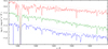 |
Fig. 1 STIS spectra of EC 11481–2303 (top, red line, flux ×1.04, for clarity), Feige 110 (middle, green), and PG0909+276 (bottom, blue). All spectra were convolved with a Gaussian (FWHM = 2 Å). The straight lines are estimates for the respective continuum-flux level. |
4 Spectral analysis
4.1 EC 11481-2303
First, we calculated an NLTE atmosphere model containing H, He, C, N, and O with TMAP, using the parameters and abundances determined by Rauch et al. (2010, Fig. 2). Then, a synthetic spectrum in the range of λ = 1140– 1709 Å was calculated. In addition to this “basic model”, an individual atmosphere model and synthetic spectrum was calculated for each of the IG elements (containing HHeCNO + IG element), where an absorption line comparison provided the rough IG-element abundance. During this procedure, parameters such as EB-V or local normalization of the continuum needed to be readjusted to achieve an optimal agreement between model and observation. At last, the final model considering HHeCNOCaScTiVCrMnFeCoNi was calculated and compared with the observation.
4.1.1 Atmospheric parameters
Teff = 55 000 ± 5000 K and log g = 5.8 ± 0.3, which were determined by Rauch et al. (2010), was confirmed. The interstellar H I column density NH I = 3.5 × 1020 cm−2 and the associated radial velocity vrad,H I = −7 km s−1 were determined by fitting the Ly α line. Additionally, the stellar radial velocity vrad = −87 km s−1 was determined, and  was obtained by the interstellar Lyman-edge fit (Fig. 3).
It must be noted, however, that for the STIS observation, better agreement was achieved for EB-V = 0.055 (reducing NH I slightly by about 15% but not having further notably impact), and was therefore adopted as such. Some interstellar absorption lines of C, N, O, Si, S, Al, and Fe were found. In contrast to previous analyses, the rotational velocity vrot (≡ v sin i) was increased from 30km s−1 to 40 km s−1 (Fig. 4), which is due to an updated adaption of the STIS resolving power, that is the spectral line spread function (Robertson 2013).
4.1.2 Abundances
The rotational broadening of atmospheric lines hampers the identification of isolated absorption lines for most identified elements. The H and He abundance determined by Rauch et al. (2010) was confirmed, hence obtaining He/H = 0.0025. [N] = −0.23 ([X] denotes log (mass fraction/solar mass fraction) of element X) was determined from several lines, such as N V λλ 1238.82, 1 242.80 Å. For C and O, upper limits were derived as no isolated absorption lines could be unambiguously identified. An upper limit of [C] < −5.45 was found with C IV λ 1548.20 Å, and [O] < −3.77 was found with the relatively weak O IV λ 1343.51 Å.
To obtain IG-element abundances, several synthetic spectra have been created (one for Cr, Mn, Fe, Co, and Ni, respectively, and one for Ca–V, as these elements exhibit fewer visible absorption lines in the investigated spectrum), whereas all other IG-elements’ lines were artificially removed. This procedure is slightly different from the above-mentioned and more practical to keep other parameters and normalization fixed. The different spectra were then compared with the observation section by section, and lines with weak blends were used for abundance fine-tuning (Fig. 5). For the elements Ca–V, few absorption lines, which all were strongly blended, could be identified, hence upper limits were determined. [Ca] < 2.66 was obtained with Ca III λ 1545.30 Å. With Sc IV λλ 1482.04, 1574.92 Å, [Sc] < 4.22 was found, with Ti V λ 1268.49 Å and Ti IV λ 1467.34 Å, [Ti] < 2.32 was determined, and using V IV λ 1395.00 Å, [V] < 2.49 was found. For Cr and Mn each, about 20 absorption lines, although partly blended, could be identified. For Fe-Ni each, about 50 absorption lines, some of which can be considered close to isolated, could be identified. The abundances were determined to [Cr] = 2.49, [Mn] = 2.80, [Fe] = 1.57, [Co] = 3.24 and [Ni] = 2.57 (Table 1). Conventionally, for the abundances an uncertainty of 0.1–0.3 dex is given. We estimate the uncertainty to be dependent on the line count n, which is proportional to the standard error of the mean  hence obtaining a lower uncertainty for Fe, Co, and Ni (factor≈ 0.63) compared to Cr and Mn.
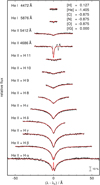 |
Fig. 2 Comparison of H and He lines of a UVES spectrum of EC 11481–2303 (black) and a model spectrum, which contains H, He, C, N, O, and a generic IG model atom (red), for the determination of Teff, log g, and He/H. The emission/absorption feature in the red wing of He II λ 4686 Å is an artifact. [X] denotes log (mass fraction/solar mass fraction) of element X. From Rauch et al. (2010), Fig. 3, modified. |
EC 11481–2303, photospheric abundances.
4.2 Feige 110
As in the case of EC 11481–2303, we started to calculate an NLTE atmosphere model containing the light metals, this time H, He, C, N, O, Si, and S, using the parameters and abundances determined by Rauch et al. (2014). Again, a synthetic spectrum in the range of λ = 1140–1709 Å was created as a basic model, and an individual atmosphere model and synthetic spectrum were calculated for each of the IG elements, where an absorption line comparison provided the rough IG-element abundance. Then, the final model considering HHeCNOSiSCaScTiVCrMnFeCoNi was calculated and compared with the observation, whereby for Feige 110, an automatic procedure was established to provide more precise IG-element abundances.
4.2.1 Atmospheric parameters
Teff = 47 250 ± 2000 K and log g = 6.0 ± 0.2, which were determined by Rauch et al. (2014), was confirmed. NH I = 2.0 × 1020 cm−2 and vrad,H I = −7 km s−1 were determined by fitting the Lyα line. vrad = −13.5 km s−1 and vrat = 0 km s−1 were determined, and EB-V = 0.02 ± 0.005 was obtained by the interstellar Lyman-edge fit. Additionally, some interstellar absorption lines of C, N, O, Si, S, Al, and Fe were found.
4.2.2 Abundances
The H and He abundances determined by Rauch et al. (2014) were confirmed, hence obtaining He/H = 0.022. [N] = −0.83 could be determined with several lines, such as NV λλ 1238.82, 1242.80 Å. [S] = −0.26 could also be derived from several lines, such as S V λλ 1268.49, 1501.76 Å. For C and O, upper limits were derived as no isolated absorption lines could be unambiguously identified. An upper limit of [C] < −6.63 was found with C IV λ 1548.20 Å, and [O] < −3.59 was found with the relatively weak O IV λ 1343.51 Å. For Si, also an upper limit was derived, as the identified absorption lines were strongly blended. Using Si IV λ 1393.76 A, [Si] < −4.1 was found.
The plethora of IG-element absorption lines leads to frequent blends. In the case of Ca, Ti, and V, few isolated absorption lines could be identified, and for Sc, none could be unambiguously identified. [Ca] = 1.32 was found with Ca III λλ 1463.34, 1545.30 Å. [Ti] = 2.47 was found with Ti IV λλ 1451.74, 1467.34 Å and [V] = 2.69 could be derived using V IV λ 1680.20 Å and V V λ 1157.58 Å. An upper limit of [Sc] < 2.64 was determined with Sc III λ 1603.06 Å. In the case of Cr–Ni, many isolated absorption lines could be identified.
To obtain more precise abundances and to investigate absorption-line properties, an automatic procedure was established with MATLAB (version 9.7.0, MATLAB 2019). As an input, the synthetic spectra calculated with TMAP, the observation, and Kurucz’s line lists (for identification of the corresponding transitions) are needed. At first, the local continuum is determined, then, for individual synthetic spectra consisting of HHeCNOSiS + IG element, all IG-element absorption lines are automatically fitted by Gaussians4, whereat line properties, such as the line center λ, the line width, and the equivalent width Wλ, are obtained. A line was considered isolated if at least 90% of its equivalent width was caused by a single transition. After some reduction, which was necessary to ensure that investigated isolated lines obtained from the synthetic spectra relate to the observed ones, the respective equivalent widths were compared (Fig. 6). More details on the procedure and the full code can be found at GitHub5.
The abundances of Cr-Ni were then adjusted until, for each of the elements, the distribution of the observed and synthetic equivalent widths,  , was equal to 1 (Fig. 7). [Cr] = 2.54, [Mn] = 2.74, [Fe] = 0.65, [Co] = 2.58, and [Ni] = 1.52 were more precisely determined this way (Table 2). Again, we estimate the uncertainty to be dependent on the line count n, that is proportional to the standard error of the mean
  .
.
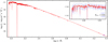 |
Fig. 3 EB–V determination for EC 11481–2303. The model flux (red) is normalized to the 2MASS Ks brightness (purple mark, bottom right). The FUSE observation is shown in gray. The insert (top right) shows a detail of the FUSE observation around 1000 A, compared to our synthetic flux attenuated with three different EB–V values. |
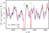 |
Fig. 4 Section of the EC 11481–2303 spectrum (STIS observation in gray, synthetic spectra in red and blue) for determination of vrot. Interstellar C II lines are indicated (index “IS”) and can be clearly distinguished due to the lack of rotational broadening. |
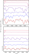 |
Fig. 5 Sections of the EC 11481–2303 spectrum (STIS observation in gray, synthetic spectra for selected element opacities are individually colored and shifted for clarity). Top: iron- and nickel-dominant section, with several weakly-blended absorption lines. Bottom: iron-dominant section. |
4.3 PG0909+276
Again, we first calculated an NLTE atmosphere model containing the light metals, this time H, He, C, N, Si, S, and Ar, using the parameters and abundances determined with an LTE model by Wild & Jeffery (2018). However, to achieve consistency of some Cin and Civ lines in the STIS spectrum, Teff had to be decreased by about 4000 K and the C abundance was reduced (Fig. 8). The newly determined values are in no worse agreement with optical spectra (Fig. 9). So, again, a synthetic spectrum in the range of λ = 1140– 1709 Å was created as a basic model, and an individual atmosphere model and synthetic spectrum was calculated for each of the IG elements, where an absorption line comparison provided the rough IG-element abundance. Then, the final model considering HHeCNSiSArCaScTiVCrMnFeCoNi was calculated and compared with the observation, whereby the above-mentioned automatic procedure was used to provide more precise IG-element abundances.
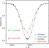 |
Fig. 6 Fev λ 1448.488 Å in the synthetic and observed spectra of Feige 110, fitted with Gaussians. The equivalent widths are indicated. |
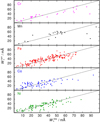 |
Fig. 7 Observed and synthetic equivalent widths of isolated Cr–Ni lines (color labeled) in Feige 110. After abundance adjustments, the values scatter around the ideal value of |

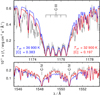 |
Fig. 8 Comparison of selected C III and C IV lines in PG 0909+276. The model of Wild & Jeſſery (2018) is shown in blue, TMAP in red, and the STIS observation in gray. |
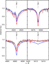 |
Fig. 9 Comparison of selected He I and He II lines in the optical spectrum of PG 0909+276. Our model with parameters by Wild & Jeſſery (2018, Teff = 36 900 K, [C] = 0.383) is shown in blue, our model with Teff = 32 900 K and [C] = 0.197 in red, and the FOCES spectrum in gray. |
4.3.1 Atmospheric parameters
Teff = 32 900 K was adopted to achieve the best match for the C lines (Fig. 8). log g = 6.1 ± 0.2 determined by Wild & Jeffery (2018) was verified. NH I = 1.1 × 1020 cm−2 and vrad,H I = 5 km s−1 were determined by fitting the Lyα line. vrad = 18.0 km s−1 and vrot ≈ 2 km s−1 were determined, and  was obtained. Additionally, some interstellar absorption lines of C, N, O, Si, S, Al, and Fe were found.
4.3.2 Abundances
The H and He abundances from Wild & Jeffery (2018) were adopted, as they provided the best fit for the optical and STIS spectrum, hence the number ratio is He/H = 0.219. As already shown, the C abundance was determined to [C] = 0.19 based on some C III and C IV lines (Fig. 8). [N] = −0.43 was found with N III λλ 1183.03, 1184.55 Å, and [Si] = −2.68 was determined with Si III λ 1298.96 Å and Si IV λλ 1393.76, 1403.77 Å. [S] = 1.22 was determined based on some S III lines, for example S III λλ 1194.46, 1200.97 Å, and S IV λλ 1623.59, 1623.95 Å, and [Ar] = 1.13 with some Ar III lines, for example Ar III λλ 1669.67, 1675.48 Å.
[Ca] = 2.00 was found using Ca III λλ 1463.34, 1496.88 Å, [Sc] = 4.24 was determined with Sc III λλ 1603.06, 1610.19 Å, and [Ti] = 2.88 was found with several lines, such as Ti IV λλ 1451.74, 1467.34 Å. [V] = 3.53 was determined with some lines, such as V III λ 1694.78 Å and V IV λ 1226.52 Å, and [Mn] = 1.98 was found with several lines, such as Mn IV λλ 1653.83, 1664.73 Å. For Cr, Fe, Co, and Ni, many isolated absorption lines were identified, hence their abundances could be more precisely determined to [Cr] = 2.51, [Fe] = 0.03, [Co] = 3.21, and [Ni] = 2.48 with the procedure described in Sect. 4.2 (Table 3). Again, the uncertainty is estimated to be proportional to the standard error of the mean  , for the line count n.
Relevant parameters for spectroscopic distance calculation.
5 Stellar parameters
With parallaxes from the Gaia data release 36 (DR3, Gaia Collaboration 2023; Babusiaux et al. 2023), stellar distances can be calculated (Bailer-Jones et al. 2021). On the other hand, spectroscopic parameters can be used to calculate the distance7, assuming the stellar radius or mass are known (Heber et al. 1984). It is then

or

with the stellar mass M in M⊙, the stellar radius R, the Edding-ton flux Hν, and the extinction-corrected apparent magnitude  (mV was taken from the NOMAD catalogue, Zacharias et al. 2004). Both equations are connected by a relation for the surface gravity g. Hν was taken from the TMAP atmosphere model (Hν = Fν/4) at λ = 5454 Å.
Taking D from Gaia DR3 and using other relevant parameters from the spectral analyses, M and R can be calculated, which provides a solid reference point for the consistency of the analysis (Table4). Interestingly, while for EC 11481–2303 the value for R is somewhat reasonable, M is relatively low, which favors log g to be at the upper end of the 1 σ error interval for a mass of M = 0.5 M⊙. The canonical hot subdwarf mass of M = 0.5 M⊙ is obtained for log g = 6.1 when fixing all other parameters at their means. For Feige 110 and PG 0909+276, obtained R and M are consistent with hot subdwarf formation theory (Heber 2016).
6 Iron-group element line strengths
Hot subdwarf spectra can be used to evaluate the quality of atomic data used as an input for the spectral analysis. Regarding the IG elements Ca–Ni, atomic data are available, for example, from NIST, the OP, or Kurucz’s line lists, whereby the latter contains by far the most data. Energy levels, cross-sections (or weighted oscillator strengths gƒ with the statistical weight g) and transition probabilities are usually determined with the help of quantum mechanical calculations. The database by Kurucz (2018) contains weighted oscillator strengths for more than 850 million LIN lines, of which approx. 330 million belong to the IG elements. Additionally, around 900 000 IG-element POS lines are available, giving a LIN/POS ratio of about 370. Kurucz uses a semi-empirical method (Kurucz 1973) to calculate the weighted oscillator strengths gƒ. However, depending on the calculation method, deviations can arise. This has already been shown by Massacrier & Artru (2012) for Sc, where for some lines large deviations (factor ≈1000 for Sc IV) were found between Kurucz’s calculations and the flexible atomic code (Gu 2002), which is a relativistic atomic configuration interaction program based on jj-coupling. Additionally, we could also show systematic deviations for the trans-iron-element (TIE) Cu IV ion between calculations by Kurucz and the Tübingen Oscillator Strength Service (TOSS8, Fig. 10), which provides oscillator strengths for 14 TIEs. For TOSS calculations, a pseudo-relativistic Hartree–Fock method with core-polarization corrections was used (Cowan 1981; Quinet et al. 1999, 2002).
As we were able to quantitatively compare line strengths between the models and the observations for a total of 457 isolated Cr–Ni lines in Feige 110 and PG 0909+276, we could use the stellar atmospheres as “laboratories” to evaluate the quality of weighted oscillator strengths gƒ for Kurucz’s POS lines. As the calculation method is the same for the LIN lines, this procedure even enables their accuracy to be tested to some extent.
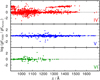 |
Fig. 10 Comparison of the calculated oscillator strengths of Cu IV – VI obtained from TOSS and Kurucz, with color labeled ions. |
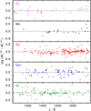 |
Fig. 11
|


7 Atomic-data quality
To estimate the statistical uncertainty σKurucz of Kurucz’s gƒ values for the investigated isolated lines, at first, the uncertainty σae of this work’s analysis and evaluation procedure and inherent assumptions needs to be known. Then, it is

where σW is the final uncertainty of the line strengths and is obtained from the distribution  from Sect. 4.2. The weighted uncertainty of 392 lines from Feige 110 and 65 lines from PG 0909+276 is σW = 49% (non-logarithmic).
σae is comprised of two components. First, approximations and possible uncertainties in the analysis procedure have to be accounted for. Second, our assumption that  is a correct measure for the deviation of a single absorption line needs to be verified. Thus, we have to investigate that
  is a correct reference value and independent from the specific stellar spectrum.
Considering the analysis procedure, 10% uncertainty was allowed when constraining the criterion for an absorption line to be isolated. Other sources of uncertainty in Sect. 4.2 might be the determination of the local continuum or non-identified line blends. Hence, we obtain a lower limit of 10% for the analysis uncertainty. Considering the uncertainty of  as a reference value, we could compare correction factors
  for absorption lines identified in both stars Feige 110 and PG 0909+276. Deviations between both stellar spectra are not attributed to analysis or atomic data uncertainties, but to the fact that
  is, for one or another reason, not a stable reference. For 21 evaluated absorption lines found in both stars (Table A.2), the statistical uncertainty amounts to 23%. Altogether, we obtain a lower limit of σae ≥ 25%.
Knowing both σW and σae, an upper limit for the statistical uncertainty of the input data can be estimated to

We emphasize that the real uncertainty (σKurucz) may be much lower. Additionally, no systematic uncertainty of Kurucz’s gƒ values was found among the investigated lines, neither when plotting  against
  (Fig. 7) nor against the wavelength (Fig.11).
8 Line-strength corrections
With the normalized distributions of equivalent widths obtained from Sect. 4.2, the deviation  for each of the isolated absorption lines in Feige 110 and PG 0909+276 could be taken as a correction factor, which in theory needed to be applied to obtain agreement between model and observation for the respective line strength (keeping in mind that this might reduce the overall uncertainty to 23%, as shown in Sect. 7, but not completely abolish it, because
  is not a stable reference). As naively a linear relationship to the equivalent width is expected, it is

for each line. The respective transitions in Kurucz’s LIN and POS lists were then corrected by substitution of gƒKurucz with g ƒcorr. Afterwards, new atmosphere models and synthetic spectra were calculated for Feige 110 and PG 0909+276 based on the new atomic data. Then, the evaluation was repeated.
As expected, this procedure significantly reduced the statistical spread of the data shown in Fig. 7 by a factor of about 1.8, which is shown in Fig. 12. However, it could not completely eradicate a spread, which hints to a more complex relation between Wλ and gƒ. From a theoretical point of view, this can be understood by stepping back from the individual transition probabilities and by having a look at a specific ion and its energy levels (with corresponding transition probabilities) as a whole, which is, for instance, described in a Grotrian diagram9. Changing oscillator strengths for specific transitions has always an impact on other transitions (as probabilities sum to unity) and therefore introduces errors.
As the consequences of these changes on the model spectrum are not yet possible to predict with the available methods, an iterative procedure would be necessary to correctly change the oscillator strength of a specific transition while not simultaneously introducing errors on other transitions. In this procedure, a specific oscillator strength would be corrected in a way that  coincide for that absorption line. Then, the atmosphere model and model spectrum need to be recalculated, correcting all the line strengths that now deviate from the original model. After a few iterations, the oscillator strength of the specific transition should be correctly adjusted and all subsequent errors should be eliminated. Then, one may proceed to the next transition, and so on. As several iterations are to be expected for each absorption line, thousands of steps would be necessary in total, which would be unacceptably time expensive, as the calculation of the atmosphere model for each step takes at least several hours.
To come back to the non-iterative procedure performed in this work, additionally to the still existing deviations after applying the corrections (Fig. 12),  become systematically too weak in Feige 110, especially for stronger lines (Fig. 12).
As those are more relevant for abundance determinations, we do not recommend such a non-iterative correction of gf values to improve statistics. In PG 0909+276 no such shift shows. As the line count is significantly larger for Feige 110, however, we still conclude that this correction procedure is not applicable.
9 Improving abundance determinations
As has been shown, corrections on weighted oscillator strengths in a non-iterative manner do not lead to an optimal agreement between models and observations, while a (probably correct) iterative procedure would be too time-expensive to be realised with the available methods. Hence, we give another recommendation to improve abundance determinations in objects similar to Feige 110 and PG 0909+276 by finding strong, isolated absorption lines with little to no deviations occurring between observed and modeled line strengths, which can serve as prime reference points for the respective element’s abundance determination. In the case of stars that are highly enriched in IG elements, as a result of which a large part of their lines overlap, statistical methods such as the χ2 method are well-suited to determine abundances. To achieve a reasonable computing time with NLTE models, however, good starting values for these abundances are important, which can only be obtained from clearly visible, isolated lines. In stars that have lower IG-element abundances, these can only be determined using a few lines anyway, which means that their accuracy is also decisive here.
Among the investigated lines, we found 58 strong, “reliable” isolated absorption lines (Table A.3) with  and
and  , which, with σae from Sect. 7, leads to an uncertainty of

per line. Typically using multiple (n) lines per element, the abundance uncertainty will reduce by a factor of  , as shown in Sect. 4.2. Depending on the analysis method, these lines can either serve as solid starting points or, if few lines are available only, the accuracy of the abundance determination can then be estimated.
10 Results and conclusions
With very high-resolution and high-S/N STIS spectra, we were able to perform an NLTE spectral analysis of the three subdwarf stars EC 11481-2303, Feige 110, and PG 0909+276.
For EC 11481-2303, the previously determined Teff = 55000 ± 5000 K and He/H = 0.0025 was confirmed by our analysis. Due to rotational broadening, many of the identified absorption lines are blended. In the case of C, O, and the IG-elements Ca–V, upper limits for the atmospheric abundances could be derived. For the other IG-elements Cr–Ni, abundances were determined.
For Feige 110, we could also confirm the previously determined Teff= 47250 ± 2000 K, log g = 6.0 ± 0.2, and He/H = 0.022. Despite the absence of rotational broadening, the plethora of IG-element absorption lines lead to frequent blends, hence for C, O, Si, and Sc, upper limits were derived. As many isolated lines were identified for Cr-Ni, an automatic method was established to determine their abundances more precisely, as well as absorption-line properties.
For PG 0909+276, we determined Teff = 32 900 K by evaluation if the C III/C IV ionization equilibrium in the STIS observation. log g = 6.1 ± 0.2 and He/H = 0.219, as previously determined, are consistent with our analysis. The abundances of all considered elements were determined, and for Cr, Fe, Co, and Ni, the above-mentioned automatic method could be used for precise abundance determination.
With the Gaia DR3 distance measurements for EC 11481-2303, we either conclude that log g is at its upper limit of log g = 6.1 or that EC11481-2303 is an unusually low-mass sdO, with  .
.
With the detailed spectral analyses of Feige 110 and PG 0909+276, we were able to investigate isolated absorption lines and compare line strengths between models and observations for a total of 457 lines, using the stellar atmospheres as laboratories to evaluate the quality of weighted oscillator strengths gf for Kurucz’s POS lines. Considering uncertainties of the analysis and the evaluation procedure, we found an upper limit for the statistical uncertainty of Kurucz’s gf values of σKurucz ≤ 0.15 dex, whereby the real uncertainty might be considerably lower.
To improve IG-element abundance determinations, we tried to apply  as a correction factor for each line’s gf. Unfortunately, although significantly reducing the statistical uncertainty, this procedure introduced a systematic shift of the equivalent widths, so that we do not recommend such a correction of gf values. Instead, to improve abundance determinations, we recommend to use strong, reliable isolated IG-element absorption lines from Table A.3 as solid starting points for a spectral analysis. These lines exhibit line-strength uncertainties of σ ≈ 27% each, whereby the abundance uncertainty significantly reduces when using multiple lines per element.
To summarize, substantial improvements could be made in the atomic data for the elements Cr, Mn, Fe, Co, and Ni in their ionization stages III–VI. We expect that all atomic data (in all ionization stages) that are calculated analogously to the Kurucz data, that were investigated on here, could be improved by a critical evaluation similar to ours.
Acknowledgements
AL had been supported by the German Aerospace Center (DLR, grant 50 OR 1704) and by the German Research Foundation (DFG, grant WE 1312/49-1). This work had been supported by the High Performance and Cloud Computing Group at the Zentrum für Datenverarbeitung of the University of Tübingen (https://www.binac.uni-tuebingen.de), the state of Baden-Württemberg through bwHPC and the German Research Foundation (DFG) through grant no. INST 37/935-1 FUGG. The TOSS service (http://astro.uni-tuebingen.de/∼TOSS), the TIRO (http://astro.uni-tuebingen.de/∼TIRO), and the TMAD tool (http://astro.uni-tuebingen.de/~TMAD) used for this work were constructed as part of the Tübingen project of the German Astrophysical Virtual Observatory (GAVO, http://www.gvo.org). This work has made use of data from the European Space Agency (ESA) mission Gaia (https://www.cosmos.esa.int/gaia), processed by the Gaia Data Processing and Analysis Consortium (DPAC, https://www.cosmos.esa.int/web/gaia/dpac/consortium). Funding for the DPAC has been provided by national institutions, in particular the institutions participating in the Gaia Multilateral Agreement. This work is based on observations made with the NASA/ESA Hubble Space Telescope obtained from the Space Telescope Science Institute, which is operated by the Association of Universities for Research in Astronomy, Inc., under NASA contract NAS 5–26555. These observations are associated with program 14746. This research has made use of NASA’s Astrophysics Data System and the SIMBAD database, operated at CDS, Strasbourg, France. We thank our unknown referee for their comments that helped us to clarify this paper.
Appendix A Additional Tables
Observation log for our program stars.
Evaluated lines in both Feige 110 and PG 0909+276, with their respective correction factors corr =  .
.
Strong, reliable IG-element absorption lines, found in Feige 110 or PG 0909+276, recommended to be employed for abundance determinations.
References
- Babusiaux, C., Fabricius, C., Khanna, S., et al. 2023, A&A, 674, A32 [NASA ADS] [CrossRef] [EDP Sciences] [Google Scholar]
- Bailer-Jones, C. A. L., Rybizki, J., Fouesneau, M., Demleitner, M., & Andrae, R. 2021, AJ, 161, 147 [Google Scholar]
- Cowan, R. D. 1981, The Theory of Atomic Structure and Spectra (Berkeley, CA: University of California Press) [Google Scholar]
- Dekker, H., D’Odorico, S., Kaufer, A., Delabre, B., & Kotzlowski, H. 2000, SPIE Conf. Ser., 4008, 534 [Google Scholar]
- Feige, J. 1958, ApJ, 128, 267 [NASA ADS] [CrossRef] [Google Scholar]
- Friedman, S. D., Howk, J. C., Chayer, P., et al. 2002, ApJS, 140, 37 [NASA ADS] [CrossRef] [Google Scholar]
- Gaia Collaboration (Vallenari, A., et al.) 2023, A&A, 674, A1 [NASA ADS] [CrossRef] [EDP Sciences] [Google Scholar]
- Green, R. F., Schmidt, M., & Liebert, J. 1986, ApJS, 61, 305 [NASA ADS] [CrossRef] [Google Scholar]
- Greenstein, J. L. 1971, in White Dwarfs, 42, ed. W. J. Luyten (Dordrecht: Reidel), 46 [NASA ADS] [CrossRef] [Google Scholar]
- Gu, M. F. 2002, ApJ, 579, L103 [CrossRef] [Google Scholar]
- Heber, U. 2016, PASP, 128, 082001 [Google Scholar]
- Heber, U., & Edelmann, H. 2004, Ap&SS, 291, 341 [NASA ADS] [CrossRef] [Google Scholar]
- Heber, U., Hunger, K., Jonas, G., & Kudritzki, R. P. 1984, in Observational Tests of the Stellar Evolution Theory, 105, eds. A. Maeder, & A. Renzini (Dordrecht: Reidel), 223 [NASA ADS] [CrossRef] [Google Scholar]
- Hubeny, I., & Mihalas, D. 2014, Theory of Stellar Atmospheres (Princeton University Press) [Google Scholar]
- Kilkenny, D., O’Donoghue, D., Koen, C., Stobie, R. S., & Chen, A. 1997, MNRAS, 287, 867 [NASA ADS] [CrossRef] [Google Scholar]
- Kudritzki, R. P. 1976, A&A, 52, 11 [NASA ADS] [Google Scholar]
- Kurucz, R. L. 1973, SAO Special Rep., 351 [Google Scholar]
- Kurucz, R. L. 1991, in NATO Advanced Study Institute (ASI) Series C, 341, Stellar Atmospheres - Beyond Classical Models, eds. L. Crivellari, I. Hubeny, & D. G. Hummer (Dordrecht: Kluwer), 441 [Google Scholar]
- Kurucz, R. L. 2018, in ASP Conf. Ser., 515, Workshop on Astrophysical Opacities, 47 [Google Scholar]
- Löbling, L., Maney, M. A., Rauch, T., et al. 2020, MNRAS, 492, 528 [Google Scholar]
- Macchetto, F. 1976, Mem. Soc. Astron. Italiana, 47, 431 [NASA ADS] [Google Scholar]
- Massacrier, G., & Artru, M. C. 2012, A&A, 538, A52 [NASA ADS] [CrossRef] [EDP Sciences] [Google Scholar]
- MATLAB 2019, version 9.7.0 (R2019b) (Natick, Massachusetts: The MathWorks Inc.) [Google Scholar]
- Naslim, N., Jeffery, C. S., Behara, N. T., & Hibbert, A. 2011, MNRAS, 412, 363 [CrossRef] [Google Scholar]
- Pfeiffer, M. J., Frank, C., Baumueller, D., Fuhrmann, K., & Gehren, T. 1998, A&AS, 130, 381 [NASA ADS] [CrossRef] [EDP Sciences] [Google Scholar]
- Quinet, P., Palmeri, P., Biémont, É., et al. 1999, MNRAS, 307, 934 [NASA ADS] [CrossRef] [Google Scholar]
- Quinet, P., Palmeri, P., Biémont, É., et al. 2002, J. Alloys Comp., 344, 255 [CrossRef] [Google Scholar]
- Ralchenko, Y., & Kramida, A. 2020, Atoms, 8, 56 [NASA ADS] [CrossRef] [Google Scholar]
- Rauch, T., & Deetjen, J. L. 2003, in ASP Conf. Ser., 288, Stellar Atmosphere Modeling, eds. I. Hubeny, D. Mihalas, & K. Werner, 103 [NASA ADS] [Google Scholar]
- Rauch, T., Werner, K., & Kruk, J. W. 2010, Ap&SS, 329, 133 [NASA ADS] [CrossRef] [Google Scholar]
- Rauch, T., Rudkowski, A., Kampka, D., et al. 2014, A&A, 566, A3 [NASA ADS] [CrossRef] [EDP Sciences] [Google Scholar]
- Rauch, T., Quinet, P., Hoyer, D., et al. 2016a, A&A, 587, A39 [NASA ADS] [CrossRef] [EDP Sciences] [Google Scholar]
- Rauch, T., Quinet, P., Hoyer, D., et al. 2016b, A&A, 590, A128 [NASA ADS] [CrossRef] [EDP Sciences] [Google Scholar]
- Riley, A. 2019, in STIS Instrument Handbook for Cycle 28 (STScI) [Google Scholar]
- Ringat, E., & Rauch, T. 2012, in ASP Conf. Ser., 452, Fifth Meeting on Hot Sub-dwarf Stars and Related Objects, eds. D. Kilkenny, C. S. Jeffery, & C. Koen, 71 [Google Scholar]
- Robertson, J. G. 2013, PASA, 30, e048 [NASA ADS] [CrossRef] [Google Scholar]
- Saffer, R. A., Bergeron, P., Koester, D., & Liebert, J. 1994, ApJ, 432, 351 [NASA ADS] [CrossRef] [Google Scholar]
- Seaton, M. J., Yan, Y., Mihalas, D., & Pradhan, A. K. 1994, MNRAS, 266, 805 [NASA ADS] [CrossRef] [Google Scholar]
- Stys, D., Slevinsky, R., Sion, E. M., et al. 2000, PASP, 112, 354 [NASA ADS] [CrossRef] [Google Scholar]
- Werner, K., Deetjen, J. L., Dreizler, S., et al. 2003, in ASP Conf. Ser., 288, Stellar Atmosphere Modeling, eds. I. Hubeny, D. Mihalas, & K. Werner, 31 [NASA ADS] [Google Scholar]
- Werner, K., Dreizler, S., & Rauch, T. 2012, Astrophysics Source Code Library [record ascl:1212.015] [Google Scholar]
- Wild, J., & Jeffery, C. S. 2017, Open Astron., 26, 246 [NASA ADS] [CrossRef] [Google Scholar]
- Wild, J. F., & Jeffery, C. S. 2018, MNRAS, 473, 4021 [CrossRef] [Google Scholar]
- Zacharias, N., Monet, D. G., Levine, S. E., et al. 2004, in Am. Astron. Soc. Meet. Abstr., 205, 48.15 [NASA ADS] [Google Scholar]
- Ziegler, M., Rauch, T., Werner, K., Köppen, J., & Kruk, J. W. 2012, A&A, 548, A109 [NASA ADS] [CrossRef] [EDP Sciences] [Google Scholar]
Although absorption lines take the shape of a Voigt profile, at least for the IG-elements, a Gaussian fit provides a very close approximation.
All Tables
Evaluated lines in both Feige 110 and PG 0909+276, with their respective correction factors corr = .
Strong, reliable IG-element absorption lines, found in Feige 110 or PG 0909+276, recommended to be employed for abundance determinations.
All Figures
|
Fig. 1 STIS spectra of EC 11481–2303 (top, red line, flux ×1.04, for clarity), Feige 110 (middle, green), and PG0909+276 (bottom, blue). All spectra were convolved with a Gaussian (FWHM = 2 Å). The straight lines are estimates for the respective continuum-flux level. |
| In the text | |
|
Fig. 2 Comparison of H and He lines of a UVES spectrum of EC 11481–2303 (black) and a model spectrum, which contains H, He, C, N, O, and a generic IG model atom (red), for the determination of Teff, log g, and He/H. The emission/absorption feature in the red wing of He II λ 4686 Å is an artifact. [X] denotes log (mass fraction/solar mass fraction) of element X. From Rauch et al. (2010), Fig. 3, modified. |
| In the text | |
|
Fig. 3 EB–V determination for EC 11481–2303. The model flux (red) is normalized to the 2MASS Ks brightness (purple mark, bottom right). The FUSE observation is shown in gray. The insert (top right) shows a detail of the FUSE observation around 1000 A, compared to our synthetic flux attenuated with three different EB–V values. |
| In the text | |
|
Fig. 4 Section of the EC 11481–2303 spectrum (STIS observation in gray, synthetic spectra in red and blue) for determination of vrot. Interstellar C II lines are indicated (index “IS”) and can be clearly distinguished due to the lack of rotational broadening. |
| In the text | |
|
Fig. 5 Sections of the EC 11481–2303 spectrum (STIS observation in gray, synthetic spectra for selected element opacities are individually colored and shifted for clarity). Top: iron- and nickel-dominant section, with several weakly-blended absorption lines. Bottom: iron-dominant section. |
| In the text | |
|
Fig. 6 Fev λ 1448.488 Å in the synthetic and observed spectra of Feige 110, fitted with Gaussians. The equivalent widths are indicated. |
| In the text | |
|
Fig. 7 Observed and synthetic equivalent widths of isolated Cr–Ni lines (color labeled) in Feige 110. After abundance adjustments, the values scatter around the ideal value of |
| In the text | |
|
Fig. 8 Comparison of selected C III and C IV lines in PG 0909+276. The model of Wild & Jeſſery (2018) is shown in blue, TMAP in red, and the STIS observation in gray. |
| In the text | |
|
Fig. 9 Comparison of selected He I and He II lines in the optical spectrum of PG 0909+276. Our model with parameters by Wild & Jeſſery (2018, Teff = 36 900 K, [C] = 0.383) is shown in blue, our model with Teff = 32 900 K and [C] = 0.197 in red, and the FOCES spectrum in gray. |
| In the text | |
|
Fig. 10 Comparison of the calculated oscillator strengths of Cu IV – VI obtained from TOSS and Kurucz, with color labeled ions. |
| In the text | |
|
Fig. 11
|
| In the text | |
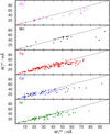 |
Fig. 12 Like Fig. 7, with corrected oscillator strengths. |
| In the text | |
Current usage metrics show cumulative count of Article Views (full-text article views including HTML views, PDF and ePub downloads, according to the available data) and Abstracts Views on Vision4Press platform.
Data correspond to usage on the plateform after 2015. The current usage metrics is available 48-96 hours after online publication and is updated daily on week days.
Initial download of the metrics may take a while.