| Issue |
A&A
Volume 548, December 2012
|
|
|---|---|---|
| Article Number | A35 | |
| Number of page(s) | 12 | |
| Section | The Sun | |
| DOI | https://doi.org/10.1051/0004-6361/201219335 | |
| Published online | 15 November 2012 | |
Solar Fe abundance and magnetic fields
Towards a consistent reference metallicity
1
Instituto de Astrofísica de Canarias (IAC),
Calle vía Láctea s/n, 38200
La Laguna, Tenerife,
Spain
e-mail: This email address is being protected from spambots. You need JavaScript enabled to view it.
; This email address is being protected from spambots. You need JavaScript enabled to view it.
; This email address is being protected from spambots. You need JavaScript enabled to view it.
2
Departamento de Astrofísica, Universidad de La Laguna
(ULL), 38205 La
Laguna, Tenerife,
Spain
3
Niels Bohr Institutet (NBI), Københavns Universitet,
Blegdamsvej 17, 2100
København Ø,
Denmark
e-mail: This email address is being protected from spambots. You need JavaScript enabled to view it.
4
Centre for Star and Planet Formation (STARPLAN), Københavns
Universitet, Øster Voldgade
5-7, 1350
København Ø,
Denmark
Received: 3 April 2012
Accepted: 20 August 2012
Abstract
Aims. We investigate the impact on Fe abundance determination of including magnetic flux in series of 3D radiation-magnetohydrodynamics (MHD) simulations of solar convection, which we used to synthesize spectral intensity profiles corresponding to disc centre.
Methods. A differential approach is used to quantify the changes in theoretical equivalent width of a set of 28 iron spectral lines spanning a wide range in wavelength, excitation potential, oscillator strength, Landé factor, and formation height. The lines were computed in local thermodynamic equilibrium (LTE) using the spectral synthesis code LILIA. We used input magnetoconvection snapshots covering 50 min of solar evolution and belonging to series having an average vertical magnetic flux density of ⟨ Bvert ⟩ = 0,50,100, and 200 G. For the relevant calculations we used the Copenhagen Stagger code.
Results. The presence of magnetic fields causes both a direct (Zeeman-broadening) effect on spectral lines with non-zero Landé factor and an indirect effect on temperature-sensitive lines via a change in the photospheric T − τ stratification. The corresponding correction in the estimated atomic abundance ranges from a few hundredths of a dex up to |Δlog ϵ(Fe)⊙| ~ 0.15 dex, depending on the spectral line and on the amount of average magnetic flux within the range of values we considered. The Zeeman-broadening effect gains relatively more importance in the IR. The largest modification to previous solar abundance determinations based on visible spectral lines is instead due to the indirect effect, i.e., the line-weakening caused by a warmer stratification as seen on an optical depth scale. Our results indicate that the average solar iron abundance obtained when using magnetoconvection models can be ~ 0.03–0.11 dex higher than when using the simpler hydrodynamics (HD) convection approach.
Conclusions. We demonstrate that accounting for magnetic flux is important in state-of-the-art solar photospheric abundance determinations based on 3D convection simulations.
Key words: magnetohydrodynamics (MHD) / radiative transfer / line: formation / Sun: abundances / Sun: granulation / Sun: photosphere
© ESO, 2012
1. Introduction
The chemical composition of stars is derived through the analysis of their emitted electromagnetic radiation. Thanks to appropriate modelling, the presence of lines of a given chemical element in the observed spectra can be interpreted in terms of its abundance in the source object. The line strength, as quantified, say, by the equivalent width, needs to be matched by the corresponding theoretical prediction. A more detailed approach involves matching the line profiles themselves instead.
As our closest star, the Sun allows the most detailed observations of the processes taking place in an object of its type. The atmospheric models used to describe the physical conditions of the solar plasma have become more and more realistic through the years, in particular, accounting for 3D inhomogeneities and for the need to have good granulation statistics. Still, magnetic fields are usually neglected in solar abundance studies, on the assumption that their effect on spectral line formation is of secondary importance. The space- and time-averaged solar spectrum commonly used for abundance determinations will in fact be weighted towards granules, owing to the larger surface area the latter cover with respect to intergranular lanes, where magnetic field concentrations tend to be found. The idea is that for this reason the impact of magnetic flux over the average emergent spectrum (and, in particular, abundances) is likely to be negligible. According to this assumption, the uncertainty introduced by using magnetic-free models would be less important than other more obvious sources of error, such as atomic data, uncertainties related to observational data, treatment of non-local thermodynamic equilibrium (non-LTE) effects, and so on. Moreover, the assumption that magnetic fields could be disregarded altogether in abundance studies has been compounded with the need of simplifying the simulation setup, spectral synthesis computations and subsequent analysis. Because of this situation, when advancing from the 1D plane-parallel approximation to a 3D approach, non-magnetic model atmospheres were used. Nevertheless, two major arguments can be put forth against that simplification.
-
1.
From an observational point of view, evidence is accumulating about a large amount of hidden magnetic flux being present in the Sun, even in “quiet” regions (see Sánchez Almeida & Martínez González 2011, for a recent review). It is now known that weak magnetic fields cover most of the Sun’s surface, with indications that a flux density of the order of 102 G may be a good reference value (Trujillo Bueno et al. 2004; Nordlund et al. 2009). In regions with strong solar magnetic fields (e.g., in plage regions), the fraction of magnetic field concentrations in intergranular lanes with 1 kG or more tends to increase (see e.g. Fig. 46 in Nordlund et al. 2009). In observed plage regions, the granulation presents a lot of fine structuring at high spatial resolution: isolated bright points, strings of bright points and dark micro-pores, “ribbons”, or more circular “flower” structures (Title et al. 1992; Berger et al. 2004; Narayan & Scharmer 2010). Granules become smaller than in the quiet areas (Muller 1977; Schmidt et al. 1988; Title et al. 1992), and intergranular lanes are characterized by the presence of micro-pores. In agreement with observations, numerical 3D convection models predict that the granulation pattern is profoundly affected in regions with high flux density (e.g. Cattaneo et al. 2003; Vögler 2005; Cheung et al. 2008), with upflowing granules of reduced size and widened intergranular lanes. In the extreme case of sunspot umbrae, the convection is seriously impaired and takes the form of narrow upflow plumes (Schüssler & Vögler 2006).
-
2.
The reasoning given for why hydrodynamics (HD) should be a good approximation for line formation in the Sun neglects the fact that the photospheric material becomes more transparent in magnetic concentrations owing to their lower density, allowing one to probe deeper, i.e., into hotter layers of the atmosphere (Stein & Nordlund 2000) where the flux tubes are also heated through heat influx from the surrounding material (Spruit 1976). Weak spectral lines will then experience brightening of their core. The weakening of neutral iron spectral lines was, for example, used by Schuessler & Solanki (1988) to predict a higher continuum intensity for magnetic elements. Observed photospheric bright points may then be identified with magnetic flux concentrations. Thus, magnetic fields can act on spectral lines not only directly, i.e., via Zeeman broadening, but also via an indirect effect associated with the temperature stratification in the line-forming regions. Only a comprehensive study using realistic 3D magnetohydrodynamical simulations can therefore confirm whether the effect of magnetic fields on spectral line formation and abundance derivation is truly negligible.
Including magnetic fields is clearly an important new step in the long-term evolution of abundance studies. Following pioneering work (e.g. Nordlund 1984), 3D radiative magnetoconvection simulations that explore realistic configurations and provide an excellent match to the photometric and spectroscopic observations were produced during the past decade, as summarized by Nordlund et al. (2009). The resulting 3D model atmospheres (albeit with zero magnetic field) have been used in abundance determination work to realistically account for the departures from homogeneity in line formation. Along with the use of better input atomic data, these advances led to remarkable agreement between the observational data and the theoretically predicted shapes and asymmetries of the spectral lines (Asplund et al. 2000a; Shchukina & Trujillo Bueno 2001), but only if decreased abundance of several chemical elements in the Sun was assumed (Asplund et al. 2000b, 2009; Asplund 2005) compared to the previously commonly adopted standard reference values inferred via a 1D static, homogeneous, and plane-parallel local thermodynamic equilibrium (LTE) analysis. The 3D-derived abundances give smaller line-to-line scatter compared to the 1D results at the same time as rendering the microturbulence and macroturbulence free parameters unnecessary. Better agreement with solar neighbourhood abundances (Lodders et al. 2009) is also obtained.
While all these results are very encouraging, pressing outstanding issues remain. Of particular importance among them is whether the neglect of magnetic fields in the convection models mentioned above has an appreciable effect on abundance determinations, a question that we approach in this paper. The role of magnetic fields in abundance determinations has been initially investigated in 1D model atmospheres (Borrero 2008), finding non-negligible effects, but it was not until very recently (Fabbian et al. 2010) that an investigation set out to study the effects in the 3D magnetohydrodynamics (MHD) case. The results of that exploratory paper indicate that, even in the magnetically quiet Sun, the neglect of magnetic fields may question the few-centidexes accuracy claimed in previous works.
In the present paper, we achieve the first comprehensive 3D study of the solar iron abundance that includes magnetic fields. We focus on iron because of the large number of spectral lines for this element in the visible and IR with different direct magnetic sensitivity (i.e., differing Landé factors gL) and also because the solar Fe abundance is the basis for most abundance work in the astrophysics literature. Iron is in fact of central historical importance as a proxy for the total metal content of a given stellar object and as the reference element in the elemental abundance ratios used in studies of galactic chemical evolution. It was claimed in the 80s that the Fe solar abundance lies anywhere between log ϵ(Fe)⊙ = 7.70 dex (Blackwell et al. 1984, 1986) and ~7.48 dex (Holweger et al. 1990). The use of 3D model atmospheres and improved observational, atomic, and modelling data led to a drastic reduction of the large line-to-line abundance scatter, whereby a low abundance of log ϵ(Fe)⊙ = 7.45 dex (Asplund et al. 2000b) was determined, consistent with the meteoritic value of Lodders et al. (2009). The question remains whether that mean value can withstand the inclusion of magnetic effects in the 3D model atmospheres by using magnetoconvection (as opposed to purely HD) models.
In this paper we find confirmation of the importance of magnetic fields in determining the solar Fe abundance. For the Fe spectral lines we have in common with Asplund et al. (2000b), we find abundance corrections of Δlog ϵ(Fe)⊙ = 0.05−0.09 dex when considering magnetoconvection models with an average unsigned magnetic flux of ⟨ Bvert ⟩ = 100 G.
The neglect of magnetic fields is not the only remaining problem in the solar abundance determination research field. Among other open questions, the most critical and urgent are (i) the friction with helioseismic inversion constraints (Antia & Basu 2005; Delahaye & Pinsonneault 2006) caused by the up to ~30% smaller estimate currently widely adopted for the solar photospheric metal content; (ii) several authors (e.g., Caffau et al. 2007, 2008, 2010, 2011; Ayres 2007, 2008) have suggested that the revision in the abundance of a number of chemical elements may be too drastic, for example due to slightly too steep temperature gradients in the employed models’ continuum-forming layers (Trujillo Bueno & Shchukina 2009) or too low temperatures in their middle photospheric layers (Ayres 2012); (iii) Caffau et al. (2009) claim that the revised solar abundances are likely to be mostly an outcome of differences in equivalent width and/or in line profile fitting, as well as in blend treatment and in atomic data, with granulation effects and hydrodynamical modelling playing a less important role.
The layout of the paper is as follows. Section 2 deals with the details of the atmospheric models employed in this study and with the method used in computing theoretical spectral line profiles. Section 3 presents the abundance correction results that we find for the different Fe lines studied here. In Sect. 4 we draw consequences specifically with respect to the solar iron content. Section 5 discusses the more general implications in terms of derivation of the elemental composition of the Sun, and Sect. 6 lists our conclusions.
2. Atmospheric models and computation of spectral lines
2.1. Method
We used simulations covering several hours of solar time that we obtained by using the 3D radiative-hydrodynamics Copenhagen STAGGER code (Galsgaard & Nordlund 1996; also, see discussion in Fabbian et al. 2010, and the recent description in Beeck et al. 2012). The simulation box covers 6.0 × 6.0 Mm2 horizontally and extends in height for ~2.8 Mm. These datacubes are divided into 252 × 126 × 252 cells, with non-uniform spacing in the vertical direction, yielding a resolution in height of  15 km at the photosphere. In the vertical direction, after avoiding the vertical ghost zones necessary in the computations, only ~2.5 Mm actually contain valuable physics information. Horizontally periodic boundary conditions are imposed for all variables on the sides of the simulation box.
The initial setup configuration for the magnetoconvection simulations is a uniform vertical magnetic field. While diverging convective upflows will tend to sweep and concentrate magnetic fields to intergranular downflow lanes (e.g., Nordlund et al. 2009), the horizontal average of the vertical component of B must remain equal at all depths and times throughout the simulation to the initial value chosen for it in the relevant series, ⟨ Bvert ⟩ = Bt = 0 = const., and thus characterizes the different magnetic series in this study. We subdivide our results into series with an initial vertical field of 0 G (i.e., the HD series) and of 50 G, of 100 G, and of 200 G (i.e., the three different MHD series). For each series we wait until a statistically stationary state has been reached, which typically takes some 0.5 solar hours after introduction of the initial vertical magnetic field. We then store snapshots of the subsequent temporal evolution at intervals of 30 s solar time.
For the a-posteriori spectral synthesis we used the LILIA code (Socas-Navarro 2001). A subdomain of the computed box extending from 425 km above to 475 km below the average τ500 nm = 1 level was used for the synthesis; the spatial resolution in that domain was increased by interpolating to a uniformly spaced grid with resolution ~7.8 km. In Fig. 1 we show the MHD-HD differences in the spatially and temporally averaged temperature stratification. The average temperature stratification is different for the different series, with a tendency in layers with log τ500 nm < 0 to an increasingly large departure from the HD temperature stratification as the initial magnetic field becomes higher, following the expected behaviour (see Sect. 1). We stress that this effect appears due to the changed opacity caused by the decreased pressure (lower density) inside strong magnetic flux concentrations (magnetic plus gas pressure being nearly equal to the gas pressure in the surrounding unmagnetized plasma, e.g. Nordlund et al. 2009). The photospheric temperature increase in MHD is therefore not related to the magnetic energy build-up by photospheric motions, which has been hypothesized to heat the corona after local release via magnetic reconnection.
The synthetic spectra were obtained only for solar disc centre. After verifying that the influence on the correspondingly derived theoretical equivalent widths was negligible, for the spectral synthesis we decreased the horizontal resolution by taking one out of every four grid points. We selected a subset of snapshots covering the last 50 min of the statistically stationary regime of convection, separated by a 150 solar seconds time interval. We therefore keep 21 snapshots per series.
Spatially- and temporally-averaged synthetic spectra were finally computed and then employed for a differential analysis of the impact of different amounts of magnetic flux on abundance determinations.
2.2. Line parameters
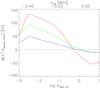 |
Fig. 1 MHD-HD difference of the temperature stratification obtained for layers close to photospheric line-forming regions after averaging horizontally on surfaces of equal optical depth and temporally over the (63 × 63 column) input snapshots used in the spectral synthesis. Blue, green and red lines represent the difference in temperature with respect to the HD case, against log 10τ(500 nm) (bottom horizontal axis), for the 50 G, 100 G and 200 G cases, respectively. The top horizontal axis shows the corresponding physical depth in Mm in the HD case. |
Atomic parameters for the 28 iron spectral lines included in the current study.
The 28 iron lines we chose for the spectral synthesis are listed (with their parameters) in Table 1. The spectral lines cover a wide range in rest wavelength (λ), with 23 of them in the visible and 5 of them in the near-IR spectral region. To detect possible dependences of the final abundance corrections on the atomic parameters, the spectral lines were chosen so as to include a wide range of values of lower transition level excitation potential (0.1 < χl < 6.5 eV), of transition oscillator strength (−5.0 < log gf < 0.4), and of Landé factor (0 ≲ gL ≲ 3). The values adopted are from the VALD (version 0.4) and NIST ASD (version 4) databases1.
In Table 1, we assign different identifiers for subgroups of lines, to reflect the organisation that is used in the discussion of results (Sect. 3). We make a division into Zeeman-insensitive (gL = 0) lines (Sect. 3.2) – identified in the table with the label “0L” – and in lines with non-zero Landé factor (Sect. 3.3). The latter are additionally subdivided into lines with high values of the Landé factor (“LL” in Table 1), i.e., having gL ≥ 1 (see Sect. 3.3.2), in lines in common with Asplund et al. (2000b) (Sect. 3.3.3) – marked in the table with “A” – and in IR lines (Sect. 3.3.4), identified with “IR”. The spectral features listed in Table 1 are all lines of neutral iron, except for the singly-ionized 611.332 nm iron line, marked in the table with “II”. The grouping just discussed will help to more clearly explain the direct and indirect effects of the magnetic flux on spectral lines.
The iron lines chosen for this study probe quite different depth ranges in the photospheric snapshots, thus jointly covering a domain from the high layers in the simulation box to as deep as around 5 km above log 10τ(500 nm) = 0. Their approximate heights of formation (e.g. see values in Gurtovenko & Kostik 1989, Table 2) make them generally safe for this study since they are supposed to be forming inside the simulation domain.
The collisional van der Waals broadening/damping formula was used following the classic approximation of Unsold (1955) with no enhancement. Our tests revealed that, while the exact choice of the enhancement factor will influence the resulting equivalent width and is thus an important choice for line profile fitting and absolute abundance matching, it does not affect a differential abundance investigation, like ours, to a significant level. For instance, the abundance correction derived from the comparison of the HD and MHD equivalent widths reduces by <0.01 dex when the enhancement factor is changed from 1.0 to 2.5.
The lines were synthesized at a spectral resolution of 0.50 pm. We found this to be a good compromise for achieving high spectral resolution at an acceptable computational effort with a resulting equivalent width accuracy better than 0.001 pm. For each spectral line, we used as many spectral points around the central wavelength as needed to reach convergence at least at the 10-2 level when calculating the equivalent width. For the strongest lines this implied using up to 1000 wavelength points (or ~250 pm on each side of the rest wavelength).
2.3. Continuum intensity
Figure 2 (top panel) shows the level of agreement between our calculated continuum intensity data (based on a space and time average for the same snapshots that were employed in the spectral synthesis) and different theoretical and measured values, all being spatially-averaged means at solar disc centre (μ = 1) and given in absolute units. Our continuum intensity results for the HD and 200 G series are seen to lie between the 3D HD values that Trujillo Bueno & Shchukina (2009) derived based on a single snapshot from Asplund et al. (2000a), and the values from the solar photospheric “thermal profiling” analysis of Ayres et al. (2006, see their Table 1. They fall in a band of ≲5% below the semiempirical model of Maltby et al. (1986), known as MACKKL, which was purposely built at the time precisely from continuum observations. Therefore, that our results are, in particular, close to the latter, confirms the goodness of our 3D MHD simulations. Our HD and MHD models also agree well with the observational data from Neckel & Labs (1984, Table VII). The bottom panel of Fig. 2 shows the intensity difference (in percentage) between our time-averaged results and the observational dataset just mentioned. The uncertainties involved in a correctly computed continuum are of the same order as the differences we find with respect to available literature constraints.
Abundance corrections for the Fe spectral lines in the visible range, for the different magnetic flux cases.
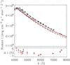 |
Fig. 2 Top panel: comparison of our computed solar disc centre continuum intensity in the non-magnetic and 200 G case (solid black and red curves, respectively) to data from the literature. The long-dashed curve is based on the results obtained by Trujillo Bueno & Shchukina (2009) using a single 3D HD snapshot by Asplund et al. (2000a); the dotted curve with circles is based on Ayres et al. (2006); the short-dashed curve refers to the semi-empirical 1D MACKKL model of the “quiet” Sun atmosphere (see Table II of Maltby et al. 1986); finally, black crosses indicate the observational data from Neckel & Labs (1984, Table VII). Bottom panel: intensity difference (in percentage) between our results and the observational data (black crosses = HD-obs; red crosses = 200 G-obs; dashed horizontal line = –5% level). |
3. Abundance correction results
3.1. Overview
The procedure used to obtain abundance corrections is as follows. From the (M)HD snapshots we obtained synthetic spectra for each of the columns in the snapshots and for all of the lines in Table 1 using a standard reference abundance value of log ϵ(Fe)⊙ = 7.50 dex (note although that the precise value adopted is not crucial here, given the differential nature of our study). Then, we calculated space and time averages (i.e., horizontally in each snapshot and for all snapshots) separately for each of the series (HD, 50 G, 100 G, 200 G). We then computed the equivalent width of the average profiles and compared the values obtained for each of the different series. Additionally, to determine abundance corrections, we ran spectral synthesis calculations for the HD case with an input Fe abundance changed by −0.10, −0.06, −0.02,+0.02, and +0.10 dex compared to the reference value mentioned above. The precise abundance correction to use in the HD case to match the equivalent width of the profiles for the MHD series was then found by interpolation between the values obtained for these fixed abundance jumps. In fact, the abundance correction to adopt as a result is actually the negative of the value obtained through the interpolation. The reason for the change of sign is that if, e.g., a given spectral line tends to weaken for non-zero magnetic flux, then when neglecting magnetic fields the equivalent width measured from observations will be matched with a lower (i.e. underestimated) elemental abundance.
Finally, to separate the magnetic broadening (Zeeman splitting) effects from the influence of the changed temperature structure in the MHD models, we ran further LILIA spectral synthesis calculations based on the MHD models (in particular, keeping the temperature and density stratification in them) but artificially setting B = 0. We expect that the line formation in this case will contain the indirect effect of the magnetically-induced temperature stratification change, but of course, without any direct Zeeman broadening.
In the following sections, we present the results of this study by dividing the spectral features in our line list into two broad groups. The first group (Sect. 3.2) contains the 13 lines with no Zeeman sensitivity (gL ~ 0), while the second group (Sect. 3.3) is composed of the 15 lines with at least some direct sensitivity (0.5 < gL ≤ 3.0) to the magnetic field.
3.2. Zeeman-insensitive spectral lines (gL = 0)
Spectral lines with gL = 0 are indicated with “0L” in Tables 1 and 2. Any magnetic effects on these lines must necessarily come from the change of temperature and density stratification alone. The magnitude of the effect then depends on the formation height and temperature sensitivity of the line. The behaviour of the calculated equivalent width with respect to magnetic flux is illustrated for two lines of this group in Fig. 3 (left and middle panels). The corresponding abundance corrections are included in Table 2, together with the predicted HD equivalent width for each spectral line (which can provide an idea of their approximate formation region, since the formation height is not available from Gurtovenko & Kostik 1989, for all lines in our list). The abundance corrections turn out to be small ( + 0.02 dex) for Fe i 423.027 nm (left panel), but reach up to ~+0.10 dex for Fe i 543.452 nm (middle panel) in the 200 G case. The radiation “feels” hotter temperatures in the MHD models. As a consequence, for a fixed adopted abundance, these spectral lines become increasingly weaker (in agreement with their temperature sensitivity), the higher the unsigned flux of the different MHD series. By checking the position of the dashed horizontal lines, we see that the abundance of the HD case must be decreased appreciably for its resulting equivalent width to match the one found for the MHD cases. Using the non-magnetic case to match measured equivalent widths from observed spectra, one would then derive a low abundance estimate. The latter will in fact allow matching predicted and measured equivalent widths because the spectral line is intrinsically stronger in HD. This finally translates into a positive abundance correction to the purely HD case, because the abundance values obtained for it must be revised upward in order to match observations while also endeavouring to account (precisely via the use of the relevant abundance correction) for the missing effects (instead naturally present in MHD) due to magnetic fields.
The other Zeeman-insensitive spectral lines in our sample all have resulting abundance corrections within the above values. For example, they reach up to only ~+0.03 dex for the Fe i 585.923 nm feature, but up to ~+0.09 dex for the 486.364 nm line.
As seen in Fig. 3 (left and middle panels), the Zeeman-insensitivity of all absorption lines in this category is confirmed by the absence of any equivalent width variation when artificially setting B = 0 in the spectral synthesis.
3.3. Spectral lines with gL ≠ 0
3.3.1. Fe II 611.3 nm line
Figure 3 (right panel) shows the equivalent width results for the only Fe ii spectral line included in this study (marked with “II” in Tables 1 and 2). The corresponding corrections to the HD-derived abundance are modest. Since Fe ii lines are weak (our predicted HD equivalent width for this line is 0.92 pm, as listed in Table 2) and generally formed rather deep in the photosphere, in the region where the temperature modifications due to the presence of magnetic fields are small (see Fig. 1), the corresponding abundance corrections can also be expected to be fairly mild. The formation height of the Fe ii 611.332 nm line lies around 110 km (see Table 2 in Gurtovenko & Kostik 1989). This line, moreover, belongs to the visible wavelength range and has a small Landé factor (gL = 0.57), so that, as seen in Fig. 3 (right panel), the Zeeman broadening is unable to contribute any significant line strengthening. The applicable abundance corrections thus settle at a maximum of ~+0.03 dex, see Table 2. Singly-ionized iron lines are generally less sensitive to temperature, to non-LTE effects and to details of the model atmosphere (see, e.g., Asplund et al. 2009). Improved atomic data for them are now available (e.g., Meléndez & Barbuy 2009). It will therefore be of future interest to ascertain, based on a larger sample of singly-ionized iron lines, whether they may also be generally insensitive to the direct and indirect effects of magnetic fields, as the results for at least Fe ii 611.332 nm seem to suggest. This would likely confirm Fe ii as a more reliable indicator than Fe i for the purpose of abundance determinations under simplified (e.g., LTE, or non-magnetic) approximations, i.e., when a more sophisticated analysis is not feasible.
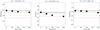 |
Fig. 3 Left and middle panels: equivalent width results for two of the Zeeman-insensitive (gL = 0) spectral lines in our line list. Right panel: equivalent width results for the Fe ii 611.332 nm spectral line. In all panels, filled circles mark the equivalent width for the (M)HD cases, with average flux density (⟨ Bvert ⟩ = Bt = 0 = const., i.e., equal throughout the evolution to its initial value) given in abscissas. Empty circles (here, essentially overlapping the filled ones) represent the equivalent width results obtained when artificially setting B = 0 for the spectral synthesis. The solid horizontal line marks the value of the equivalent width for the HD case. The dashed horizontal lines mark the equivalent width value obtained when decreasing the iron abundance of the HD model by 0.02,0.06, and 0.10 dex. |
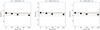 |
Fig. 4 Equivalent width results for three of the gL > 1 spectral features in our line list. The symbols are the same as in Fig. 3 (but now filled and empty circles are no longer overlapping). |
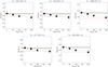 |
Fig. 5 Equivalent width results for the spectral lines in common with Asplund et al. (2000b). Same symbols as in Fig. 3. |
3.3.2. Lines with large Landé factor gL
Spectral lines with gL ≥ 1 are indicated with “LL” in Tables 1 and 2. The abundance corrections for these lines are given in Table 2, together with their predicted HD equivalent width. Figure 4 shows the equivalent width results for three spectral features with large gL, namely the 630.150 nm, 630.249 nm, and 525.064 nm lines. The abundance corrections for these lines are of intermediate magnitude, reaching the value ~+0.05 dex, ~+0.06 dex, and ~+0.08 dex, respectively. Given their non-zero Zeeman sensitivity, the equivalent width of all three lines decreases when artificially setting B = 0 for the spectral synthesis, as seen in the figure. However, this effect remains small throughout the visible range, showing that magnetic broadening is not sufficient to counter the indirect line-weakening temperature effect.
Some of the lines marked as A or IR in Table 1 also have a large Landé factor gL. However, they are discussed as separate subgroups below, because they are helpful for highlighting some of the main results of this study, i.e. the possible impact on the accepted value of the solar iron abundance and the more noticeable Zeeman broadening effects in the IR.
3.3.3. Lines in common with the solar iron abundance study of Asplund et al. (2000)
Figure 5 shows the equivalent width results for the spectral features marked with “A” in Tables 1 and 2. We include them in an own separate subgroup, given that they are the ones in common with a previous well-known solar Fe abundance study (Asplund et al. 2000b). Corresponding abundance corrections and HD equivalent widths are listed in Table 2. These spectral lines have some of the largest Landé factors among the visible lines in our sample. However, since all five are in the visible range, Zeeman broadening actually has small influence on them and can do only little to alleviate the line weakening tendency, as is apparent by comparing the empty and filled circles in Fig. 5. On the other hand, their sensitivity to the magnetically induced changes in the average temperature stratifications is high, placing these spectral features among those in our line list that have the largest abundance corrections (see Table 2). Namely, for the 200 G case, the corresponding correction to the HD-derived abundance is between 0.08 dex for the 608.271 nm line to 0.14 dex for the 524.705 nm one, which is the maximum, the latter being the largest effect in the whole sample we studied. Fe i 525.021 nm (the spectral line that, together with Fe i 524.703 nm, made up the “good magnetic pair” of Stenflo 1973) has the second most significant corrections, Δlog ϵ(Fe)⊙ = 0.12 dex for the 200 G case. Apart from having been used in the solar iron abundance derivation of Asplund et al. (2000b), this line has also recently been targeted by the IMaX imaging vector magnetograph instrument (Martínez Pillet et al. 2011; Bonet et al. 2010) onboard the ballon-borne Sunrise telescope mission (Barthol et al. 2011; Solanki et al. 2010).
3.3.4. IR lines
Spectral iron lines belonging to the infrared wavelength range are identified with “IR” in Table 1. Table 3 lists their abundance corrections and HD equivalent widths. All of the IR lines included in our line list are strong, 7.6 < WHD < 19.9 pm. Figure 6 shows the relevant equivalent width results. As seen, these lines behave like those in the visible concerning their sensitivity to the warmer temperature structure in the MHD models. However, the IR iron lines we selected have quite large Landé factors. Coupled with the λ2 dependence of Zeeman broadening, this makes them prone to strong direct magnetic effects. The net result is that, compared to the HD case, these IR iron lines tend to generally become stronger in the MHD models. The corresponding abundance corrections range from negligible to −0.08 dex.
4. Consequences concerning the solar Fe abundance
Different neutral and/or ionized iron lines should yield a consistent estimate for the photospheric solar abundance. Once using appropriately weigthed averaging of the abundance values inferred from the various spectral lines of a given chemical element, little scatter should in fact result around the “best estimate”. In this section, we provide average values for the abundance correction to be applied to different groups of lines. In doing so, we just conform to the usual practice in the literature whereby averages of abundance values from multiple spectral lines have been routinely taken as the representative derived solar abundance. Since there is no obvious way to attach a different statistical significance to the abundance correction obtained for each line, we simply give equal weight to them when calculating averages.
Abundance corrections for the five IR spectral lines of Fe i included in this study.
Spectral lines in the visible: as can be seen in Table 2, the abundance corrections for the lines in the visible range vary from negligible to as high as +0.14 dex. The unweighted mean of the corrections for these lines is shown in Table 2 in the row near the bottom marked with ⟨ ⟩ signs, and it varies between 0.02 and 0.06 dex when going from the 50 G to the 200 G case. If we focus on the visible Fe lines marked with “A” in our table (i.e., those in common with Asplund et al. 2000b), we find that they yield significantly higher abundance values when MHD modelling is used. In detail, out of these five spectral lines, Fe i 608.271 nm is the least affected, with abundance corrections of 0.02–0.08 dex, depending on the magnetic flux considered. The most affected is Fe i 524.705 nm, with abundance corrections of 0.04–0.14 dex.
We may apply the average abundance correction values (given in the row marked with ⟨ ⟩ ∗ in Table 2) to the abundance determinations by Asplund et al. (2000b) for those five lines. The average value found by them with an HD treatment was log ϵ(Fe)⊙ = 7.42 ± 0.03. We would then obtain an average solar iron abundance estimate in the range 7.45 ≤ log ϵ(Fe)⊙ ≤ 7.53 dex, depending on the magnetic flux assumed. On the other hand, even if we apply abundance corrections separately for the different lines following the results in Table 2 and calculate the mean value and rms, the value of the latter turns out to be close to the one calculated using purely HD models. In detail: the rms is 0.03 dex for the 50 G case and 0.04 dex for the 100 and 200 G cases, hence very similar to the values obtained by Asplund et al. (2000b). Therefore, the good line-to-line agreement found by those authors is not spoilt when the MHD approach is considered.
Spectral lines in the IR: the average value of the abundance corrections for the IR iron lines we studied is indicated in Table 3 (bottom row, marked with ⟨ ⟩). We derive a negative average correction in the range −0.02 < ⟨ Δlog ϵ(Fe)⊙ ⟩ < −0.04 dex. However, the scatter around the mean is quite large for these lines, because of the scatter in their Landé factor (see Table 1) and the relative importance that the Zeeman effect has for each of these IR lines.
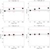 |
Fig. 6 Equivalent width results for the IR spectral lines included in our sample. The symbols are the same as in Fig. 3, except that now, the dashed horizontal lines indicate the equivalent width value predicted when increasing the iron abundance in the HD model by 0.02 and 0.10 dex. This translates to negative abundance corrections of the same magnitude applicable to the abundance predicted using the HD model (see discussion in text). |
5. Discussion
First results using a 3D MHD approach to abundance analysis were presented in our previous paper (Fabbian et al. 2010), where the study was limited to three iron lines. Here, we have aimed at extending those exploratory results using a much larger set of spectral lines, which allowed us to further improve the constraints on the relevant derived effects on the solar abundance. However, it is important to note that, given the differential nature of our study, it is not our main aim to match the exact value of measured equivalent widths. Despite this, with the input solar iron abundance we adopted for the spectral synthesis and using a sensible choice of magnetic flux, we find generally good agreement between our predicted MHD equivalent widths and those from observational data available in the literature for lines marked “A” in our Table 2 (e.g., the value by Holweger et al. 1995, for the 624.065 nm line and the values by Blackwell et al. 1995, for the four remaining lines). In all cases we find that it is indeed appropriate to consider a magnetic flux in the range ⟨ Bvert ⟩ ~ 50−200 G at the corresponding depths of line formation in the real Sun.
Photospheric Fe lines in the solar case have the property that their strength decreases with increasing temperature in their formation layers (see Gray 1992); thus, the hotter average stratification caused by the presence of magnetic concentrations tends to decrease their predicted equivalent widths with respect to the HD case. The direct (i.e., Zeeman) effect acts in the opposite direction. In the visible range, the former effect dominates and systematically smaller equivalent widths result. In the IR, Zeeman broadening is important and stronger lines (i.e., larger equivalent widths than in the HD case) may result as a net effect.
A dual picture thus clearly emerges from our results. For spectral lines in the visible wavelength range (Figs. 3–5), Zeeman broadening is relatively small and the dominant influence of magnetic fields on line formation is the line-weakening effect of the warmer average temperature structure in the revelant line-formation layers of MHD model atmospheres (see Fig. 1). The 3D HD abundance results will need to be amended via positive abundance corrections to increase their value to the one appropriate to the magnetic case considered most representative of solar conditions. On the other hand, Zeeman splitting becomes important in the IR region of the spectrum and where it tends to be able to more than compensate for the indirect line-weakening effect, so much so that for lines with particularly high Zeeman sensitivity (gL > 1.5, top panels of Fig. 6), a net line-strengthening effect is noticeable. The 3D HD abundance will in this case need to be revised downward (i.e., applying negative corrections to it).
These results are in line with our previous exploratory findings (Fabbian et al. 2010). A cross-check can be made since the three lines in that paper are included in the current study. The agreement is very good. Any small difference in the theoretical equivalent width or in the derived abundance corrections (generally in the sense of slightly more significant effects having been found now) are due to better spectral sampling and continuum coverage in the present study. We chose to decrease the number of snapshots and the spatial subsampling employed compared to our previous study, only after having made sure that this did not have a significant impact on the equivalent width of the lines.
To confirm that the physical processes involved can explain the effects we found, we checked for any trend of the abundance corrections versus the parameters characterizing the line formation, namely, rest wavelength of the line, lower level excitation potential and oscillator strength of the given transition, level multiplicity (2s+1) and total angular momentum J, line centre formation height, Landé factor, and HD line strength. Here we present a figure (Fig. 7) corresponding to the only clear trend retrievable, namely that the sign of the abundance correction tends to reverse as one moves from wavelengths in the visible λ range to the IR. In Fig. 7 we have exceptionally included results for a few lines of elements other than iron. These are C i 477.590 nm, O i 615.818 nm, Ni i 676.777 nm (used in SOHO MDI magnetogram images), Mn i 874.091 nm, Si i 1082.71 nm (this IR line is the strongest in the sample we study, i.e., having an equivalent width >500 mÅ), and finally, Mn i 1526.27 nm (Asensio Ramos 2009; Asensio Ramos et al. 2009). We consider these additional lines of other elements because, as shown in Fig. 7, they cover the region of intermediate wavelengths in the visible to near-IR where our sample has no iron lines, and provide hints that magnetic flux acts similarly also on lines of different elements than iron. Interestingly, the lines of the other elements in fact follow a similar trend to the one seen for iron lines. This would seem to suggest that the effects encountered can be generalized to other elements according to considerations on a given line’s formation height and temperature sensitivity, on the one hand, and Landé factor and wavelength, on the other. We also see that the percentage change in equivalent width decreases smoothly from the lower to the upper wavelengths range limits for those lines.
In general, we find significant differences in the effects for different lines. Correspondingly, the abundance corrections vary from quite small ( dex) to significant (up to |Δlog ϵ(Fe)⊙| ~ 0.15 dex in the 200 G case) for all but a few of the spectral lines analysed. Lines affected to a level at or above 0.02 dex represent a majority, for the magnetic series we here investigated only rare exceptions.
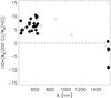 |
Fig. 7 Equivalent width percentage change of the 200 G case compared to HD, plotted against line rest wavelength. Filled diamonds are for the 28 iron lines listed in Table 1, empty symbols for 6 lines of other elements which were used to complement our line list and for testing. |
We focussed also on the subset of lines that we have in common with the absolute solar iron abundance determination of Asplund et al. (2000b). These all have gL ≥ 1. The abundance corrections found here for them are among the most significant of those we find to be applicable to the lines we have studied. Interestingly, for this subset of lines, the effects due to the presence of magnetic fields can be seen as linked to their formation height. That is, they follow the trend seen in Fig. 1, according to which lines formed between a height of 200 and 400 km feel increasingly strong indirect effects. The abundance corrections for lines in this subset follow the trend expected, based on their formation heights (see values in Gurtovenko & Kostik 1989, Table 2). Other spectral features used in the study by Asplund et al. (2000b) are also likely to be affected by significant abundance corrections, in particular for lines with a small Landé factor, for which the indirect effect found here can act undisturbed. Thus, the last word on the solar iron photospheric abundance has probably not yet been spoken.
Our results also urge more investigation into the magnitude of the magnetic effects for other chemical elements than iron. In particular, this is true for those elements whose abundances have in the last decade undergone a revision that has caused large disagreement between standard solar models and helioseismology constraints. It is crucial that also oxygen, carbon, neon, nitrogen, and silicon – i.e. those elements playing a major role in determining the total solar metallicity Z/X – be redetermined via targeted studies simultaneously including the most accurate atomic and observational data and non-LTE, 3D, and magnetic effects.
Since all spectral lines have a more or less pronounced sensitivity to the temperature values of the layers where they are formed, and since direct magnetic sensitivity of the lines, if present, induces line broadening, one can make a broad division into the following expected general behaviour, depending on the chemical element and ionization stage considered:
-
Spectral lines for which magnetic broadening acts in the opposite sense to the indirect temperature effect. This is the case of both neutral and singly-ionized iron lines in the Sun and of other elements having the same temperature sensitivity. In this category, there will be some rare instances of close-to-negligible net abundance corrections. In general, though, the direct and the indirect effect will not balance out exactly. The net resulting abundance correction can be either positive or negative, with a sign inversion expected when moving from UV to IR wavelengths, i.e., towards the spectral range where Zeeman broadening becomes important.
-
Spectral lines for which the indirect temperature effect acts in the same direction as magnetic broadening. These will tend to become stronger in MHD simulations, thus the relevant abundance corrections to be applied to 3D HD abundance determinations will always be negative. Still, their magnitude should be investigated on a case-by-case basis. The net abundance corrections will be maximized, because of the direct and indirect effects working together to reinforce the spectral line. Although Zeeman splitting for most lines of chemical elements other than iron may not be as important, the spectral features in this category will still tend to become stronger in the warmer MHD temperature stratification thanks to the indirect effect. One important example are lines of neutral oxygen (since that chemical element remains mostly neutral in the solar photosphere due to its much higher ionization potential compared to e.g. iron), for which our preliminary abundance results of work included in an upcoming publication seem to indicate significant effects.
Given the differential nature of our investigation, we expect that the inclusion of non-LTE effects on Fe i lines should not change our conclusions significantly. If anything, non-LTE corrections for neutral iron are expected to push the solar abundance determination even higher due to over-ionization caused by the near-UV radiation field, hence producing under-population of the neutral iron atomic levels corresponding to the relevant transitions and thus to weaker emergent line profiles compared to LTE due to line opacity deficit (Collet et al. 2005; Shchukina & Trujillo Bueno 2001). In fact, attempts at improving the 3D HD LTE-based Asplund et al. (2000b) study also in this sense have already pushed the solar iron abundance back up to log (Fe)⊙ = 7.50, while achieving better agreement with helioseismology, and while preserving the agreement between values based on lines from neutral and singly-ionized Fe and the small line-to-line scatter and absence of trends with excitation potential (see Table 1 and Fig. 6 in Asplund et al. 2009). Based on that result and on our current findings regarding the systematic abundance corrections due to the presence of magnetic fields (with likely additional effects expected in full 3D non-LTE, see Holzreuter & Solanki 2012), the real photospheric solar iron content may well be log (Fe)⊙ > 7.50, i.e. in a relatively high range compared to the best estimates obtained in the past decade. A less “anemic” Sun would better agree with new, accurate determinations of the solar Si content accounting for non-LTE effects (Shchukina & Sukhorukov 2012; Shchukina et al. 2012).
Both of these changes, together with hints that 3D-based revisions in other chemical elements may seemingly not need to be drastic compared to the 1D case (e.g., see the results of Caffau et al. 2009, based on CO5BOLD 3D granulation models), should help alleviate the discomfort that helioseismology has been feeling towards low values of the solar metal content. In any case, it will be very interesting to investigate how 3D, non-LTE, and magnetic effects interact, and whether there may be some amplification or reduction in their magnitude when looking at a fully consistent picture in order to carry out an absolute abundance determination.
A further remaining uncertainty revolves around choosing the MHD model that is thought to best represent the real Sun, in order to estimate the most appropriate abundance correction to be applied to the abundance derived in the HD case. In particular, further testing of the realism of the MHD models must be carried out in terms of geometric configuration and depth profile of the magnetic field. Our non-magnetic model has significantly lower values of the photospheric temperature for the average stratification at log τ500 nm < 0 compared with the temperature structure of the semi-empirical solar atmosphere derived by Holweger & Mueller (1974). For those same optical depths, our MHD models are progressively closer to it as magnetic flux is increased, while very good agreement is generally reached for deep layers. Compared to the theoretical results of Stein & Nordlund (1998, see their Fig. 15, also shown in Fig. 14 of Nordlund et al. 2009), our HD atmospheric temperatures achieve similar to significantly better agreement (in photospheric and deep layers, respectively) with the stratification of Holweger & Mueller (1974). A number of observational results are certainly helping to constrain the possibilities, and comparisons with future, high-quality, targeted solar data are set to improve this scenario even further. In this sense, we have embarked on a detailed comparison and testing in terms of line parameters and thermodynamics, of centre-to-limb variation (CLV) and Stokes parameters, as well as of line fitting and absolute abundance derivation, but this goes beyond the scope of the present paper and is part of work in progress. As an example, the tests we carried out and discuss in a separate article (Beck et al. 2012) show that the agreement with the observational data we studied of predicted properties (for spatially- and spectrally-degraded spectral lines), such as the rms fluctuations at different line depression levels of bisector position/velocity, bisector intensity, and line width, may at least in some cases improve when including magnetic fields in the simulations. It will also be important to continue along the line traced by initial efforts of using Stokes spectra from magnetoconvection simulations (Stein et al. 2011) to make comparison possible of theoretical predictions with the best available current and future spectropolarimetric observational data.
6. Conclusions
We have demonstrated that appreciable effects on a set of iron spectral lines are found when introducing magnetic fields in 3D, time-dependent radiation-hydrodynamics simulations of solar surface convection. Even the most advanced chemical composition studies so far, using 3D convection modelling, may still be affected in a significant way in terms of metallicity determinations owing to their non-magnetic assumption. We here determined the associated abundance corrections to be applied when abundances are derived via a purely HD approach. In the following, we briefly highlight our main findings.
We have presented evidence that the magnetic field causes both Zeeman broadening in the lines with non-zero Landé factors and also changes in the average temperature stratification seen on an optical depth scale. Since the majority of the lines have non-zero Landé factors and are also temperature-sensitive to some extent, no spectral line is in principle exempt from relevant abundance corrections. The effects are therefore ubiquitous. The direct (line-strengthening) effect of magnetic field on line formation via Zeeman broadening is generally (except in the IR) less important in magnitude than the indirect effect of temperature stratification changes.
The abundance corrections are approximately proportional to the average unsigned magnetic field strength ⟨ |Bvert| ⟩ . For ⟨ Bvert ⟩ = 100 G, the abundance corrections are |Δlog (Fe)| ~ 0.04 dex for our full selection of iron spectral lines in the visible wavelength range and |Δlog (Fe)| ~ 0.07 dex for the subgroup in common with Asplund et al. (2000b).
If, as a number of recent results seem to suggest, the “quiet” solar photosphere is in fact teeming with hidden magnetic flux, the abundance of iron based on HD modelling will need to be revised upwards. It is likely that a more accurate estimate for the solar iron content may be log (Fe) ≳ 7.50.
The Vienna Atomic Line Database (VALD) is available as an online interface at http://vald.astro.univie.ac.at/~vald/php/vald.php; the National Institute of Standards and Technology Atomic Spectra Database (NIST ASD) is accessible at http://www.nist.gov/pml/data/asd.cfm
Acknowledgments
We gratefully acknowledge financial support by the European Commission through the SOLAIRE Network (MTRN-CT-2006-035484), by the Spanish Ministry of Research and Innovation through projects AYA2007-66502, CSD2007-00050, AYA2007-63881, and AYA2011-24808, and by the Danish Research Agency – Danish Natural Science Research Council. We acknowledge the computing time granted through the DEISA SolarAct and PRACE SunFlare projects and the corresponding use of the HLRS and FZJ-JSC JUROPA supercomputer installations, as well as the computing time allocated via RES calls at the MareNostrum (BSC/CNS, Spain) and LaPalma (IAC/RES, Spain) supercomputers. We also appreciate the use of the facilities at the Danish Center for Scientific Computing (DCSC-KU, Denmark). We thank the referee for helpful comments and A. de Vicente (IAC Condor management), H. Socas-Navarro, N. Shchukina, J. Trujillo Bueno, C. Beck, C. Allende-Prieto, and J. M. Borrero for fruitful interaction.
References
- Antia, H. M., & Basu, S. 2005, ApJ, 620, L129 [NASA ADS] [CrossRef] [Google Scholar]
- AsensioRamos, A. 2009, ApJ, 690, 416 [NASA ADS] [CrossRef] [Google Scholar]
- Asensio Ramos, A., Martínez González, M. J., López Ariste, A., Trujillo Bueno, J., & Collados, M. 2009, in Solar Polarization 5: In Honor of Jan Stenflo, eds. S. V. Berdyugina, K. N. Nagendra, & R. Ramelli, ASP Conf. Ser., 405, 215 [Google Scholar]
- Asplund, M. 2005, ARA&A, 43, 481 [NASA ADS] [CrossRef] [Google Scholar]
- Asplund, M., Nordlund, Å., Trampedach, R., Allen de Prieto, C., & Stein, R. F. 2000a, A&A, 359, 729 [NASA ADS] [Google Scholar]
- Asplund, M., Nordlund, Å., Trampedach, R., & Stein, R. F. 2000b, A&A, 359, 743 [NASA ADS] [Google Scholar]
- Asplund, M., Grevesse, N., Sauval, A. J., & Scott, P. 2009, ARA&A, 47, 481 [NASA ADS] [CrossRef] [Google Scholar]
- Ayres, T. R. 2007, in BAAS, 38, AAS Meeting Abstracts, 842 [Google Scholar]
- Ayres, T. R. 2008, ApJ, 686, 731 [NASA ADS] [CrossRef] [Google Scholar]
- Ayres, T. R. 2012, in AAS Meeting Abstracts, 219, #144.08 [Google Scholar]
- Ayres, T. R., Plymate, C., & Keller, C. U. 2006, ApJS, 165, 618 [NASA ADS] [CrossRef] [Google Scholar]
- Barthol, P., Gandorfer, A., Solanki, S. K., et al. 2011, Sol. Phys., 268, 1 [NASA ADS] [CrossRef] [Google Scholar]
- Beck, C., Fabbian, D., Moreno-Insertis, F., Puschmann, K. G., & Rezaei, R. 2012, submitted [Google Scholar]
- Beeck, B., Collet, R., Steffen, M., et al. 2012, A&A, 539, A121 [NASA ADS] [CrossRef] [EDP Sciences] [Google Scholar]
- Berger, T. E., Rouppe van der Voort, L. H. M., Löfdahl, M. G., et al. 2004, A&A, 428, 613 [NASA ADS] [CrossRef] [EDP Sciences] [Google Scholar]
- Blackwell, D. E., Booth, A. J., & Petford, A. D. 1984, A&A, 132, 236 [NASA ADS] [Google Scholar]
- Blackwell, D. E., Booth, A. J., Haddock, D. J., Petford, A. D., & Leggett, S. K. 1986, MNRAS, 220, 549 [NASA ADS] [CrossRef] [Google Scholar]
- Blackwell, D. E., Lynas-Gray, A. E., & Smith, G. 1995, A&A, 296, 217 [NASA ADS] [Google Scholar]
- Bonet, J. A., Márquez, I., Sánchez Almeida, J., et al. 2010, ApJ, 723, L139 [NASA ADS] [CrossRef] [Google Scholar]
- Borrero, J. M. 2008, ApJ, 673, 470 [NASA ADS] [CrossRef] [Google Scholar]
- Caffau, E., Steffen, M., Sbordone, L., Ludwig, H.-G., & Bonifacio, P. 2007, A&A, 473, L9 [NASA ADS] [CrossRef] [EDP Sciences] [Google Scholar]
- Caffau, E., Ludwig, H.-G., Steffen, M., et al. 2008, A&A, 488, 1031 [CrossRef] [EDP Sciences] [Google Scholar]
- Caffau, E., Ludwig, H.-G., & Steffen, M. 2009, Mem. Soc. Astron. Italiana, 80, 643 [Google Scholar]
- Caffau, E., Ludwig, H.-G., Bonifacio, P., et al. 2010, A&A, 514, A92 [NASA ADS] [CrossRef] [EDP Sciences] [Google Scholar]
- Cattaneo, F., Emonet, T., & Weiss, N. 2003, ApJ., 588, 1183 [NASA ADS] [CrossRef] [MathSciNet] [Google Scholar]
- Cheung, M. C. M., Schüssler, M., Tarbell, T. D., & Title, A. M. 2008, ApJ, 687, 1373 [NASA ADS] [CrossRef] [Google Scholar]
- Collet, R., Asplund, M., & Thévenin, F. 2005, A&A, 442, 643 [NASA ADS] [CrossRef] [EDP Sciences] [MathSciNet] [Google Scholar]
- Delahaye, F., & Pinsonneault, M. H. 2006, ApJ, 649, 529 [NASA ADS] [CrossRef] [Google Scholar]
- Fabbian, D., Khomenko, E., Moreno-Insertis, F., & Nordlund, Å. 2010, ApJ, 724, 1536 [NASA ADS] [CrossRef] [Google Scholar]
- Galsgaard, K., & Nordlund, Å. 1996, J. Geophys. Res., 101, 13445 [NASA ADS] [CrossRef] [Google Scholar]
- Gray, D. F. 1992, The observation and analysis of stellar photospheres, Camb. Astrophys. Ser., 20 [Google Scholar]
- Gurtovenko, E. A., & Kostik, R. I. 1989, Fraunhofer Spectrum and a system of Solar Oscillator Strengths [Google Scholar]
- Holweger, H., & Mueller, E. A. 1974, Sol. Phys., 39, 19 [NASA ADS] [CrossRef] [Google Scholar]
- Holweger, H., Heise, C., & Kock, M. 1990, A&A, 232, 510 [NASA ADS] [Google Scholar]
- Holweger, H., Kock, M., & Bard, A. 1995, A&A, 296, 233 [NASA ADS] [Google Scholar]
- Holzreuter, R., & Solanki, S. K. 2012, A&A, 547, A46 [NASA ADS] [CrossRef] [EDP Sciences] [Google Scholar]
- Lodders, K., Palme, H., & Gail, H.-P. 2009, in Landolt-Börnstein – Group VI Astronomy and Astrophysics Numerical Data and Functional Relationships in Science and Technology Volume, ed. J. E. Trümper, 44 [Google Scholar]
- Maltby, P., Avrett, E. H., Carlsson, M., et al. 1986, ApJ, 306, 284 [Google Scholar]
- Martínez Pillet, V., Del Toro Iniesta, J. C., Álvarez-Herrero, A., et al. 2011, Sol. Phys., 268, 57 [NASA ADS] [CrossRef] [Google Scholar]
- Meléndez, J., & Barbuy, B. 2009, A&A, 497, 611 [NASA ADS] [CrossRef] [EDP Sciences] [Google Scholar]
- Muller, R. 1977, Sol. Phys., 52, 249 [NASA ADS] [CrossRef] [Google Scholar]
- Narayan, G., & Scharmer, G. B. 2010, A&A, 524, A3 [NASA ADS] [CrossRef] [EDP Sciences] [Google Scholar]
- Neckel, H., & Labs, D. 1984, Sol. Phys., 90, 205 [NASA ADS] [CrossRef] [Google Scholar]
- Nordlund, A. 1984, in ESA SP 220, eds. T. D. Guyenne, & J. J. Hunt, 37 [Google Scholar]
- Nordlund, Å., Stein, R. F., & Asplund, M. 2009, Liv. Rev. Sol. Phys., 6, 2 [Google Scholar]
- Sánchez Almeida, J., & Martínez González, M. 2011, in Solar Polarization 6, eds. J. R. Kuhn, D. M. Harrington, H. Lin, S. V. Berdyugina, J. Trujillo-Bueno, S. L. Keil, & T. Rimmele, ASP Conf. Ser., 437, 451 [Google Scholar]
- Schmidt, W., Grossmann-Doerth, U., & Schroeter, E. H. 1988, A&A, 197, 306 [NASA ADS] [Google Scholar]
- Schuessler, M., & Solanki, S. K. 1988, A&A, 192, 338 [NASA ADS] [Google Scholar]
- Schüssler, M., & Vögler, A. 2006, ApJ, 641, L73 [NASA ADS] [CrossRef] [Google Scholar]
- Shchukina, N., & Trujillo Bueno, J. 2001, ApJ, 550, 970 [NASA ADS] [CrossRef] [Google Scholar]
- Shchukina, N., Sukhorukov, A., & Trujillo Bueno, J. 2012, ApJ, 755, 176 [NASA ADS] [CrossRef] [Google Scholar]
- Shchukina, N. G., & Sukhorukov, A. V. 2012, Kinematics and Physics of Celestial Bodies, 28, 49 [NASA ADS] [CrossRef] [Google Scholar]
- Socas-Navarro, H. 2001, in Advanced Solar Polarimetry – Theory, Observation, and Instrumentation, ed. M. Sigwarth, ASP Conf. Ser., 236, 487 [Google Scholar]
- Solanki, S. K., Barthol, P., Danilovic, S., et al. 2010, ApJ, 723, L127 [NASA ADS] [CrossRef] [Google Scholar]
- Spruit, H. C. 1976, Sol. Phys., 50, 269 [NASA ADS] [CrossRef] [Google Scholar]
- Stein, R. F., & Nordlund, A. 1998, ApJ, 499, 914 [Google Scholar]
- Stein, R. F., & Nordlund, Å. 2000, Sol. Phys., 192, 91 [NASA ADS] [CrossRef] [Google Scholar]
- Stein, R. F., Georgobiani, D., Nordlund, A., & Lagerfjard, A. 2011, in AAS/Solar Physics Division Abstracts, #42, 804 [Google Scholar]
- Stenflo, J. O. 1973, Sol. Phys., 32, 41 [NASA ADS] [CrossRef] [Google Scholar]
- Title, A. M., Topka, K. P., Tarbell, T. D., et al. 1992, ApJ, 393, 782 [NASA ADS] [CrossRef] [Google Scholar]
- Trujillo Bueno, J., & Shchukina, N. 2009, ApJ, 694, 1364 [NASA ADS] [CrossRef] [Google Scholar]
- Trujillo Bueno, J., Shchukina, N., & Asensio Ramos, A. 2004, Nature, 430, 326 [Google Scholar]
- Unsold, A. 1955, Physik der Sternatmospharen, MIT besonderer Berucksichtigung der Sonne [Google Scholar]
- Vögler, A. 2005, Mem. Soc. Astron. It., 76, 842 [NASA ADS] [Google Scholar]
All Tables
Abundance corrections for the Fe spectral lines in the visible range, for the different magnetic flux cases.
Abundance corrections for the five IR spectral lines of Fe i included in this study.
All Figures
|
Fig. 1 MHD-HD difference of the temperature stratification obtained for layers close to photospheric line-forming regions after averaging horizontally on surfaces of equal optical depth and temporally over the (63 × 63 column) input snapshots used in the spectral synthesis. Blue, green and red lines represent the difference in temperature with respect to the HD case, against log 10τ(500 nm) (bottom horizontal axis), for the 50 G, 100 G and 200 G cases, respectively. The top horizontal axis shows the corresponding physical depth in Mm in the HD case. |
| In the text | |
|
Fig. 2 Top panel: comparison of our computed solar disc centre continuum intensity in the non-magnetic and 200 G case (solid black and red curves, respectively) to data from the literature. The long-dashed curve is based on the results obtained by Trujillo Bueno & Shchukina (2009) using a single 3D HD snapshot by Asplund et al. (2000a); the dotted curve with circles is based on Ayres et al. (2006); the short-dashed curve refers to the semi-empirical 1D MACKKL model of the “quiet” Sun atmosphere (see Table II of Maltby et al. 1986); finally, black crosses indicate the observational data from Neckel & Labs (1984, Table VII). Bottom panel: intensity difference (in percentage) between our results and the observational data (black crosses = HD-obs; red crosses = 200 G-obs; dashed horizontal line = –5% level). |
| In the text | |
|
Fig. 3 Left and middle panels: equivalent width results for two of the Zeeman-insensitive (gL = 0) spectral lines in our line list. Right panel: equivalent width results for the Fe ii 611.332 nm spectral line. In all panels, filled circles mark the equivalent width for the (M)HD cases, with average flux density (⟨ Bvert ⟩ = Bt = 0 = const., i.e., equal throughout the evolution to its initial value) given in abscissas. Empty circles (here, essentially overlapping the filled ones) represent the equivalent width results obtained when artificially setting B = 0 for the spectral synthesis. The solid horizontal line marks the value of the equivalent width for the HD case. The dashed horizontal lines mark the equivalent width value obtained when decreasing the iron abundance of the HD model by 0.02,0.06, and 0.10 dex. |
| In the text | |
|
Fig. 4 Equivalent width results for three of the gL > 1 spectral features in our line list. The symbols are the same as in Fig. 3 (but now filled and empty circles are no longer overlapping). |
| In the text | |
|
Fig. 5 Equivalent width results for the spectral lines in common with Asplund et al. (2000b). Same symbols as in Fig. 3. |
| In the text | |
|
Fig. 6 Equivalent width results for the IR spectral lines included in our sample. The symbols are the same as in Fig. 3, except that now, the dashed horizontal lines indicate the equivalent width value predicted when increasing the iron abundance in the HD model by 0.02 and 0.10 dex. This translates to negative abundance corrections of the same magnitude applicable to the abundance predicted using the HD model (see discussion in text). |
| In the text | |
|
Fig. 7 Equivalent width percentage change of the 200 G case compared to HD, plotted against line rest wavelength. Filled diamonds are for the 28 iron lines listed in Table 1, empty symbols for 6 lines of other elements which were used to complement our line list and for testing. |
| In the text | |
Current usage metrics show cumulative count of Article Views (full-text article views including HTML views, PDF and ePub downloads, according to the available data) and Abstracts Views on Vision4Press platform.
Data correspond to usage on the plateform after 2015. The current usage metrics is available 48-96 hours after online publication and is updated daily on week days.
Initial download of the metrics may take a while.