| Issue |
A&A
Volume 547, November 2012
|
|
|---|---|---|
| Article Number | A100 | |
| Number of page(s) | 19 | |
| Section | Cosmology (including clusters of galaxies) | |
| DOI | https://doi.org/10.1051/0004-6361/201219646 | |
| Published online | 06 November 2012 | |
Redshift-space correlation functions in large galaxy cluster surveys
1
Institut de Physique Théorique, CEA Saclay,
91191
Gif-sur-Yvette,
France
e-mail: This email address is being protected from spambots. You need JavaScript enabled to view it.
2
Max-Planck-Institut für extraterrestrische Physik (MPE),
Giessenbachstrasse
1, 85748
Garching,
Germany
Received:
22
May
2012
Accepted:
10
September
2012
Abstract
Context. Large ongoing and upcoming galaxy cluster surveys in the optical, X-ray and millimetric wavelengths will provide rich samples of galaxy clusters at unprecedented depths. One key observable for constraining cosmological models is the correlation function of these objects, measured through their spectroscopic redshift.
Aims. We study the redshift-space correlation functions of clusters of galaxies, averaged over finite redshift intervals, and their covariance matrices. Expanding as usual the angular anisotropy of the redshift-space correlation on Legendre polynomials, we consider the redshift-space distortions of the monopole as well as the next two multipoles, 2ℓ = 2 and 4.
Methods. Taking into account the Kaiser effect, we developed an analytical formalism to obtain explicit expressions of all contributions to these mean correlations and covariance matrices. We include shot-noise and sample-variance effects as well as Gaussian and non-Gaussian contributions.
Results. We obtain a reasonable agreement with numerical simulations for the mean correlations and covariance matrices on large scales (r > 10 h-1 Mpc). Redshift-space distortions amplify the monopole correlation by about 10−20%, depending on the halo mass, but the signal-to-noise ratio remains of the same order as for the real-space correlation. This distortion will be significant for surveys such as DES, Erosita, and Euclid, which should also measure the quadrupole 2ℓ = 2. The third multipole, 2ℓ = 4, may only be marginally detected by Euclid.
Key words: surveys / galaxies: clusters: general / large-scale structure of Universe / cosmology: observations
© ESO, 2012
1. Introduction
The growth of structure in our Universe results from a competition between gravitational attraction and the mean Hubble expansion. Studying recent structures provides an understanding of both these phenomena along with supplementary insights into the initial conditions that describe primordial density fluctuations, which are assumed to be nearly Gaussian-distributed. Analyses of massive large galaxy surveys (Cole et al. 2005; Moles et al. 2008; Eisenstein et al. 2011; Blake et al. 2011b), galaxy cluster surveys (Böhringer et al. 2001; Burenin et al. 2007; Koester et al. 2007a; Vanderlinde et al. 2010; Mehrtens et al. 2012), weak-lensing studies (e.g. Benjamin et al. 2007; Massey et al. 2007; Kilbinger et al. 2009; Schrabback et al. 2010), and measurements of the baryonic acoustic oscillation peak (Eisenstein et al. 2005; Blake et al. 2011a; Slosar et al. 2011) are currently under way or are planned to probe the physics of large scales in multiple complementary ways.
Clusters of galaxies are defined as galaxy concentrations, but they can also be regarded as a specific class of objects in their own right. In the hierarchical framework of structure formation, they are the largest and last nonlinear objects in a quasi-equilibrium state. Observationally, they are well-defined and are systematically identified as strong X-ray emitters, thanks to their hot gas phase (e.g. Sarazin 1988; Pierre et al. 2011), and/or as isolated (red) galaxy overdensities (Abell 1958; Koester et al. 2007b), and/or via their imprint on the cosmological background radiation (Sunyaev & Zeldovich 1972; Planck Collaboration 2011; Reichardt et al. 2012). Observed clusters are much more rare than individual galaxies (current cluster surveys amount up to a few tens of objects per deg2), but the link to their parent dark matter halo mass is better understood. Most of cluster cosmological studies rely on the abundance of clusters and its evolution (Borgani et al. 2001; Rozo et al. 2010; Mantz et al. 2010; Sehgal et al. 2011; Clerc et al. 2012). However, very large ongoing surveys (e.g. Pierre et al. 2011) or planned surveys (Predehl et al. 2009; Refregier et al. 2011) promise to overcome the statistical limit and better constrain cosmological models by stuyding the spatial clustering of clusters over large volumes.
This work follows our previous study (Valageas et al. 2011, hereafter Paper I) that analytically quantified covariance matrices for correlation functions in the framework of large galaxy cluster surveys. These calculations are essential to account for uncertainties in clustering analyses. Most generally, these uncertainties combine a shot-noise term (arising from the discreteness of the objects) and a sample variance term (due to the finite volume of the Universe being surveyed), as well as mixed contributions. All are related to the survey design and we applied our formalism to predict signal-to-noise ratios for observable quantities given different survey strategies (Pierre et al. 2011; Valageas et al. 2011). We presented our method in a way as close as possible to observational analyses, e.g. refering to the widely-used Landy-Szalay estimator for the two-point correlation function, integrated within fixed distance bins, averaging over all accessible redshift values, etc. Our results were found to agree well with large N-body simulations. However, only real-space comoving coordinates were considered, i.e., we ignored halo peculiar velocities. Because their radial component impacts object distance measurements via an additional spectral redshift, these peculiar velocities distort the correlation function estimates.
The goal of the present paper is to estimate the corrections induced by these redshift-space distortions, still considering galaxy clusters only, and to predict if these effects may be observed in present and future cluster surveys. Indeed, redshift-space distortion measurements have attracted growing interest as a cosmological probe. Schematically, this can be understood as follows: because peculiar velocities are linked to the gravitational well created by surrounding matter, bulk flows in the large scale structure are directly linked to the growth rate of structures. More precisely, redshift-space distortions are sensitive to D+(a), the linear growth factor, as a function of cosmic scale-factor a, and to f = dlnD+/dlna. In particular, observational results have been obtained by various galaxy spectroscopic surveys such as the 2dFGRS (Peacock et al. 2001), the SDSS (Cabré & Gaztañaga 2009; Reid et al. 2012), 2dF-SDSS LRG and QSO survey (Ross et al. 2007), and the VVDS Guzzo et al. (2008).
In the following, we assume galaxy clusters to have been detected individually in a dedicated survey (e.g. in the X-ray band) and their redshift to have been subsequently determined, e.g. by measurements of their member galaxy spectra and averaging over the corresponding galaxy redshifts. This is the most common – but observationally expensive – method to determine cluster redshifts. In practical applications, only a subsample of all cluster members can be observed due to observational constraints (limiting magnitude, compactness of the cluster in the instrumental focal plane, finite wavelength range of the spectrograph, identification of spectral lines, elimination of fore- and background objects, etc.). This translates into statistical errors on the cluster redshift estimate (e.g. Katgert et al. 1996; Adami & Ulmer 2000). Most generally, spectroscopic redshifts of galaxy clusters are considered to be precise to σ(z) ~ 0.01(1 + z) or less.
To distinguish measurement errors from intrinsic covariances, we assume cluster redshifts to be known with infinite accuracy and neglect any kind of bias. Adding these sources of noise (which are not correlated with the shot-noise and sample-variance terms that we consider here) is not difficult as one only needs to add the relevant covariance matrices. We do not consider this second step here, which depends on the details of the instrument.
As in Paper I, we considered in our calculations the effects of shot-noise and sample variance. We expanded the angular anisotropy of the redshift-space correlation function on Legendre polynomials. Our formalism then leads to expressions for the monopole and the two multipoles 2ℓ = 2 and 2ℓ = 4. We provide explicit expressions for the expected quantities and their covariance matrices, taking into account the Kaiser effect and Gaussian as well as non-Gaussian contributions. Keeping in mind the application to galaxy cluster surveys, all quantities were integrated within the 0 < z < 1 redshift range. Halos were defined by their mass M and we describe the population by using a mass function and a bias model from previous works. The three- and four-point correlation function were estimated by means of a hierarchical model (Peebles 1980; Bernstein 1994), where those quantities only depend on combinations of two-point correlation functions. Comparisons with numerical simulations were made to assess the reliability of our analytical calculations.
Therefore, our main improvements over previous works consist in the inclusion of Gaussian and non-Gaussian contributions in the computation of covariance matrices, as well as in the derivation of observables close to those expected in practical studies focused on galaxy clusters.
This paper is organized as follows. In Sect. 2 we first briefly describe the analytic models that we used to estimate the means and covariance matrices of redshift-space halo correlation functions, as well as the numerical simulations that we used to check our results. Then, focusing on the Landy & Szalay estimator, we study the means of the various multipoles of the redshift-space correlation in Sect. 3, and their covariance matrices in Sect. 4. We compare our analytical results with numerical simulations for the two lowest multipoles (the “2ℓ = 0” monopole and the “2ℓ = 2” quadrupole). We apply our formalism to several real surveys in Sect. 5, for the three multipoles generated by the Kaiser effect (2ℓ = 0,2, and 4). We conclude in Sect. 6.
We give details of our calculations in Appendices A and B, and we show the auto- and cross-correlation matrices of the “2ℓ = 2” multipole in Appendix C.
2. Redshift-space halo density field
Before we describe our analysis of the covariance matrices for halo number counts and correlation functions, we present in this section the analytic models that we used for the underlying halo distributions (mass function and bias, etc.) and the numerical simulations that we used to validate our results.
2.1. Analytic models
To be consistent with the numerical simulations, we use the WMAP3 cosmology in Sects. 3 and 4 where we develop our formalism and compare our results with simulations, that is, Ωm = 0.24, Ωde = 0.76, Ωb = 0.042, h = 0.73, σ8 = 0.77, ns = 0.958, and wde = −1 (Spergel et al. 2007). In Sect. 5, where we apply our formalism to obtain forecasts for current and future surveys, we use the more recent WMAP7 cosmology (Komatsu et al. 2011), that is, Ωm = 0.274, Ωde = 0.726, Ωb = 0.046, h = 0.702, σ8 = 0.816, ns = 0.968, and wde = −1.
Keeping in mind the study of X-ray clusters, we considered the number counts and correlations of dark matter halos defined by the nonlinear density contrast δ = 200. These halos are fully characterized by their mass, and we did not investigate the relationship between this mass and cluster properties such as the gas temperature and X-ray luminosity. These scaling laws can be added to our formalism to derive the cluster number counts and correlations, depending on the quantities that are actually measured, but we kept a more general setting in this paper.
2.1.1. Halo mass function and bias
We use the halo mass function,
dn/dlnM, of Tinker et al. (2008), and the halo bias,
b(M), of Tinker
et al. (2010). Then, we write the two-point real-space correlation function
between two halos labeled “i” and “j” as  (1)where
ξ is the real-space matter density correlation. This corresponds to
the halo power spectrum
(1)where
ξ is the real-space matter density correlation. This corresponds to
the halo power spectrum  (2)where
P(k) is the matter density power spectrum. Here we
used the approximation of scale-independent halo bias, which is valid to better than 10%
on scales
20 < x < 130 h-1 Mpc
(Manera & Gaztanaga 2011), with a small
feature on the baryon acoustic scale
(r ~ 100 h-1 Mpc) of amplitude of 5%
(Desjacques et al. 2010).
(2)where
P(k) is the matter density power spectrum. Here we
used the approximation of scale-independent halo bias, which is valid to better than 10%
on scales
20 < x < 130 h-1 Mpc
(Manera & Gaztanaga 2011), with a small
feature on the baryon acoustic scale
(r ~ 100 h-1 Mpc) of amplitude of 5%
(Desjacques et al. 2010).
To simplify notations, we define the mean cumulative number density
 of objects
observed at a given redshift, within the mass bin
[M−,M+] ,
as
of objects
observed at a given redshift, within the mass bin
[M−,M+] ,
as  (3)and the mean bias
 as
as
 (4)In the following we
omit to write the explicit boundaries on mass since we only consider a single mass bin.
It is straightforward to extend all our results to the case of several mass bins by
writing the relevant mass boundaries and replacing factors such as
(4)In the following we
omit to write the explicit boundaries on mass since we only consider a single mass bin.
It is straightforward to extend all our results to the case of several mass bins by
writing the relevant mass boundaries and replacing factors such as
 by
by
 .
.
2.1.2. Redshift-space correlation functions
We denote by x and s
real-space and redshift-space coordinates. They only differ by their radial component
because of the peculiar velocity along the line-of-sight,  (5)Here,
ez is the unit vector
along the line of sight and v the peculiar velocity. At
linear order, the peculiar velocity field and the density contrast are related in
Fourier space as
(5)Here,
ez is the unit vector
along the line of sight and v the peculiar velocity. At
linear order, the peculiar velocity field and the density contrast are related in
Fourier space as  (6)where
D+ is the linear growing mode. From the conservation of
matter,
(1 + δ(s))ds = (1 + δ)dx,
one obtains the redshift-space matter power spectrum (Kaiser 1987)
(6)where
D+ is the linear growing mode. From the conservation of
matter,
(1 + δ(s))ds = (1 + δ)dx,
one obtains the redshift-space matter power spectrum (Kaiser 1987)  (7)where
 (8)Here and in the
following, we use a superscript (s) for redshift-space quantities.
Following common practice, we assume that the halo velocity field is not biased. This
yields at the same order the redshift-space halo power spectrum
(8)Here and in the
following, we use a superscript (s) for redshift-space quantities.
Following common practice, we assume that the halo velocity field is not biased. This
yields at the same order the redshift-space halo power spectrum 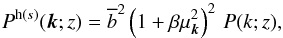 (9)with
 , where
is the
mean bias of the halo population as defined in Eq. (4) (Percival & White
2009). We write the associated redshift-space halo correlation function as
, where
is the
mean bias of the halo population as defined in Eq. (4) (Percival & White
2009). We write the associated redshift-space halo correlation function as
 (10)where
ξ(s)(s) can
be expanded as (Hamilton 1992)
(10)where
ξ(s)(s) can
be expanded as (Hamilton 1992) 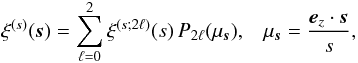 (11)where we
introduced the functions
(11)where we
introduced the functions 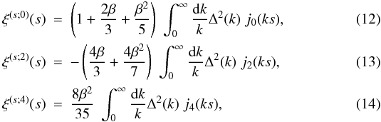 where
jℓ are the spherical Bessel functions and
we introduced the logarithmic power
Δ2(k) = 4πk3P(k).
where
jℓ are the spherical Bessel functions and
we introduced the logarithmic power
Δ2(k) = 4πk3P(k).
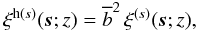
The function ξ(s) and its multipoles ξ(s;2ℓ) depend on the halo population through the factor β (i.e., the bias cannot be fully factored out as in the real-space correlation (1)). However, it is convenient to introduce the auxiliary function ξ(s) as in Eq. (10) so that most expressions obtained in the following have the same form as in real space (which is recovered by setting β = 0, that is, ξ(s) = ξ).
Independently of the linear-order approximation (9), only even multipoles can appear in the expansion (11) because of parity symmetry in redshift-space. Nonlinear corrections may add higher-order even multipoles that could be handled by a straightforward generalization of the approach developed in this paper.
The redshift-space distortions (9) and (11) only include the “Kaiser effect” (Kaiser 1987), associated with large-scale flows (i.e., the collapse of overdense regions and the expansion of underdense regions), which amplifies the power because the density and velocity fields are closely related as in Eq. (6). However, on smaller scales within virialized regions, there appears a high velocity dispersion that adds a decorrelated random component to relation (5). This yields the so-called “fingers of God” (Jackson 1972) that can be seen on galaxy surveys and give a damping factor to their redshift-space power spectrum. In this paper we focus on cluster surveys where this effect does not arise (as can be checked in numerical simulations, Nishimichi & Taruya 2011). Indeed, because clusters are the largest nonlinear objects, cluster pairs are still in the process of moving closer (or farther appart in fewer cases) and have not had time to fall within a common potential well and develop a high velocity dispersion through several orbital revolutions. Therefore, we only need to consider the Kaiser effect as in Eqs. (9) and (11). This provides a good agreement with numerical simulations for s > 20 h-1 Mpc (within 10%, except for the multipole 2ℓ = 4, which shows stronger deviations from linear theory, Reid & White (2011), but we will see that this multipole is not very important for cluster studies), and for k < 0.1 h Mpc-1 in Fourier space (Percival & White 2009; Nishimichi & Taruya 2011).
We assume that these expressions still provide a good approximation up to the weakly nonlinear scales that are relevant for studies of cluster correlations (≳ 6 h-1 Mpc). For numerical purposes we use the popular fitting formula to numerical simulations of Smith et al. (2003) for the matter power spectrum.
Nevertheless, the formalism that we develop in the following sections is fully general and does not rely on Eqs. (12)−(14) and the truncation of the series (11) at 2ℓ = 4. It can be applied to any model for the redshift-space correlation ξ(s)(s). If this leads to higher-order multipoles ξ(s;2ℓ), one simply needs to extend the sums to all required multipoles in the various expressions given in Appendix A.
2.1.3. Three-point and four-point halo correlations
The covariance matrices of estimators of the halo two-point correlation involve the
three-point and four-point halo correlations. Therefore, we need a model for these
higher-order correlations. As in Valageas et al.
(2011), following Bernstein (1994), Szapudi & Colombi (1996), and Meiksin & White (1999), we use a hierarchical
ansatz (Groth & Peebles 1977; Peebles 1980) and we write the real-space halo
three-point correlation ζh as ![Mathematical equation: \begin{equation} \label{zeta-def} \zetah_{1,2,3} = b_1 b_2 b_3 \; \frac{S_3}{3} \; \left[ \xi_{1,2} \xi_{1,3} + \xi_{2,1} \xi_{2,3} + \xi_{3,1} \xi_{3,2} \right] , \end{equation}](/articles/aa/full_html/2012/11/aa19646-12/aa19646-12-eq82.png) (15)where we sum over all
three possible configurations over the three halos labeled “1”, “2”, and “3”, and the
real-space halo four-point correlation ηh as
(15)where we sum over all
three possible configurations over the three halos labeled “1”, “2”, and “3”, and the
real-space halo four-point correlation ηh as ![Mathematical equation: \begin{eqnarray} \label{eta-def} \etah_{1,2,3,4} & = & b_1 b_2 b_3 b_4 \; \frac{S_4}{16} \; \left[ \xi_{1,2} \xi_{1,3} \xi_{1,4} + 3 \, {\rm cyc.} \right. \nonumber \\ && \left. + \xi_{1,2} \xi_{2,3} \xi_{3,4} + 11 \, {\rm cyc.} \right] , \end{eqnarray}](/articles/aa/full_html/2012/11/aa19646-12/aa19646-12-eq84.png) (16)where
“3 cyc.” and “11 cyc.” stand for three and eleven terms that are obtained from the
previous one by permutations over the labels “1, 2, 3, 4” of the four halos. As in Valageas et al. (2011), we take for the normalization
factors S3 and S4 their
large-scale limit, which is obtained by perturbation theory (Peebles 1980; Fry 1984; Bernardeau et al. 2002b),
(16)where
“3 cyc.” and “11 cyc.” stand for three and eleven terms that are obtained from the
previous one by permutations over the labels “1, 2, 3, 4” of the four halos. As in Valageas et al. (2011), we take for the normalization
factors S3 and S4 their
large-scale limit, which is obtained by perturbation theory (Peebles 1980; Fry 1984; Bernardeau et al. 2002b),  where
n is the slope of the linear power spectrum at the scale of interest.
The model (15)−(18) is the simplest model that qualitatively
agrees with large-scale theoretical predictions (which also give the scalings
ζ ~ ξ2 and
η ~ ξ3, but where the normalization
factors S3 and S4 show an
additional angular dependence) and small-scale numerical results (Colombi et al. 1996) (which however show an additional moderate
scale-dependence of the normalization factors S3 and
S4). As shown in Valageas
et al. (2011), this model (15)−(18) provides reasonably
good predictions for the covariance matrices of estimators of the cluster two-point
correlations (which focus on weakly nonlinear scales).
where
n is the slope of the linear power spectrum at the scale of interest.
The model (15)−(18) is the simplest model that qualitatively
agrees with large-scale theoretical predictions (which also give the scalings
ζ ~ ξ2 and
η ~ ξ3, but where the normalization
factors S3 and S4 show an
additional angular dependence) and small-scale numerical results (Colombi et al. 1996) (which however show an additional moderate
scale-dependence of the normalization factors S3 and
S4). As shown in Valageas
et al. (2011), this model (15)−(18) provides reasonably
good predictions for the covariance matrices of estimators of the cluster two-point
correlations (which focus on weakly nonlinear scales).
Next, for the redshift-space correlations ζh(s) and ηh(s) we use the same hierarchical ansatz (15)−(16), where in the right-hand-side we replace ξ by the redshift-space two-point correlation ξ(s) given in Eq. (11). This redshift-space model has not been checked in details against numerical simulations in previous works and we compare our predictions with simulations in Sect. 4 below. We will check that it yields a reasonable agreement for covariance matrices (especially along the diagonal) as for our purposes we only need a simple and efficient approximation. If one aims at predicting the three-point and four-point redshift-space correlations for their own sake, up to a high accuracy, one should perform dedicated tests for these quantities and probably build more sophisticated models, but this is beyond the scope of this paper.
This approximation allows us to extend in a straightforward fashion the formalism developed in Valageas et al. (2011) to redshift-space estimators. The only difference comes from the angular dependence of the two-point correlation (11), that is, from the second and fourth spherical harmonics ξ(s;2)(s)P2(μ) and ξ(s;4)(s)P4(μ). In particular, as clearly seen in Eq. (9), by setting β = 0, which only leaves the monopole contribution ℓ = 0, we recover the real-space results given in Valageas et al. (2011).
2.2. Numerical simulations
To check our analytical model, we compare our predictions with the numerical simulations that we used in Valageas et al. (2011) for real-space statistics. While we had considered only real-space coordinates in our previous study, we used the peculiar velocity assigned to each halo to conduct our comparison in redshift-space coordinates.
Here we briefly recall the main characteristics of these simulations. We used the high-resolution, all-sky, “horizon” simulation run (Teyssier et al. 2009). It consists of a (2 h-1 Gpc)3N-body simulation carried out with the RAMSES code (Teyssier 2002). The effect of baryons is neglected and the total number of particles in the simulation sets the total mass of the simulation. The mass resolution, which is the mass of each of the 40963 simulated particules, is ~1010 M⊙. Halos are found using the HOP algorithm (Eisenstein & Hut 1998). The (real-space) comoving position and peculiar velocity of each halo are obtained by averaging over all particles making up its total mass. Comoving coordinates are further transformed into sky positions (two angles plus redshift) and redshift-space coordinates taking into account their radial velocity. To ensure completeness of the simulation in all directions, we only considered halos at z < 0.8.
Simulated surveys are extracted from the full-sky light-cone catalog by defining non-overlapping rectangular regions in angular coordinates. Each field covers an area of 50 deg2. To minimize correlations between neighboring fields, we required a separation of 20 deg between two consecutive surveys, which results in a total of 34 such independent fields distributed all across the sky. Only for the results discussed in Sect. 4.3 we also used a 10 deg gap (resulting in 138 fields). For the purpose of deriving the correlation function, auxiliary random fields were created by shuffling the angular coordinates of halos in the original data fields. This operation preserves the original redshift and mass distribution of the simulation. The density of objects in the random fields was increased to one hundred times that of original data fields to avoid introducing spurious noise. The Landy-Szalay estimator and its generalization (see Sect. 3.1, Eq. (20)) provide an estimate of the two-point correlation and its multipoles in redshift space. As in Valageas et al. (2011), the mean and covariance of all derived quantities were finally estimated by sample averaging over the extracted fields.
3. Mean redshift-space two-point correlation functions
Since we have in mind the application to cluster surveys and, more generally, to deep surveys of rare objects, we considered 3D correlation functions averaged over a wide redshift bin (to accumulate a large enough number of objects), rather than the usual local 3D correlation functions at a given redshift. This means that the quantities that we considered, while being truly 3D correlations and not 2D angular correlations, nevertheless involve integrations along the line of sight within a finite redshift interval. We followed the formalism and the notations of Valageas et al. (2011) to derive the means and the covariance matrices of estimators of these integrated redshift-space correlations.
3.1. Analytical results
We focus on the Landy & Szalay estimator of the two-point correlation Landy & Szalay (1993), given by 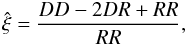 (19)where
D represents the data field and R an independent
Poisson distribution, both with the same mean density. In practice, before appropriate
rescaling, the mean number density of the Poisson process R is actually
taken to be much higher than the observed one, so that the contribution from fluctuations
of the denominator RR to the noise of
(19)where
D represents the data field and R an independent
Poisson distribution, both with the same mean density. In practice, before appropriate
rescaling, the mean number density of the Poisson process R is actually
taken to be much higher than the observed one, so that the contribution from fluctuations
of the denominator RR to the noise of
 can be ignored. The advantage of Eq. (19)
is that one automatically includes the geometry of the survey (including boundary effects,
cuts, etc.), because the auxiliary field R is drawn on the same geometry.
In practice, our generalization of the estimator (19) to redshift-space multipoles writes as
can be ignored. The advantage of Eq. (19)
is that one automatically includes the geometry of the survey (including boundary effects,
cuts, etc.), because the auxiliary field R is drawn on the same geometry.
In practice, our generalization of the estimator (19) to redshift-space multipoles writes as 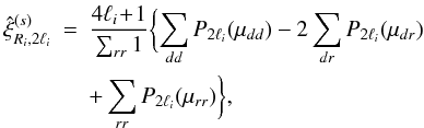 (20)where
each sum counts all the pairs, dd,dr, or rr, within the
samples D and R, that are separated by a redshift-space
distance s within the bin
Ri, − < s < Ri, +.
Compared with the usual monopole estimator (19), we added the geometrical weight
(4ℓi + 1)P2ℓi(μ)
to each pair in the numerator while in the denominator we kept the unit weight. Of course,
for ℓi = 0 we recover Eq. (19).
(20)where
each sum counts all the pairs, dd,dr, or rr, within the
samples D and R, that are separated by a redshift-space
distance s within the bin
Ri, − < s < Ri, +.
Compared with the usual monopole estimator (19), we added the geometrical weight
(4ℓi + 1)P2ℓi(μ)
to each pair in the numerator while in the denominator we kept the unit weight. Of course,
for ℓi = 0 we recover Eq. (19).
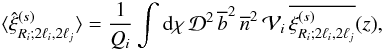
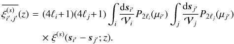
Within our framework, we write this estimator  ,
for the multipole 2ℓi of the mean correlation
on scales delimited by Ri, − and
Ri, +, integrated over some redshift range
and mass interval, as
,
for the multipole 2ℓi of the mean correlation
on scales delimited by Ri, − and
Ri, +, integrated over some redshift range
and mass interval, as 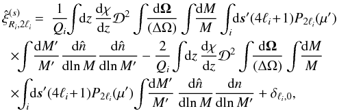 (21)with
 (22)Here
we denoted
∫ids′ as
the integral
(22)Here
we denoted
∫ids′ as
the integral  over the 3D
spherical shell i, of inner and outer radii
Ri, − and
Ri, + in redshift-space,
μ′ = (ez·s′)/s′
is the cosine of the angle between the line of sight and the halo pair,
χ(z) and
over the 3D
spherical shell i, of inner and outer radii
Ri, − and
Ri, + in redshift-space,
μ′ = (ez·s′)/s′
is the cosine of the angle between the line of sight and the halo pair,
χ(z) and  are the comoving radial and angular distances,
δℓi,0
is the Kronecker symbol (which is unity if
ℓi = 0 and zero otherwise), and
are the comoving radial and angular distances,
δℓi,0
is the Kronecker symbol (which is unity if
ℓi = 0 and zero otherwise), and
 is the observed density of objects. Here and in the following, we note observed quantities
by a hat (i.e., in one realization of the sky) to distinguish them from mean quantities,
such as the mean comoving number density
dn/dlnM. The two subscripts
Ri and
2ℓi label the radial bin and the
multipole. If we consider NR radial bins and
Nℓ multipoles, there are
NR × Nℓ
values of the index i (i.e., two different indices i and
j may correspond to different radial bins and multipoles, or to the
same radial bin but with two different multipoles, and vice versa).
is the observed density of objects. Here and in the following, we note observed quantities
by a hat (i.e., in one realization of the sky) to distinguish them from mean quantities,
such as the mean comoving number density
dn/dlnM. The two subscripts
Ri and
2ℓi label the radial bin and the
multipole. If we consider NR radial bins and
Nℓ multipoles, there are
NR × Nℓ
values of the index i (i.e., two different indices i and
j may correspond to different radial bins and multipoles, or to the
same radial bin but with two different multipoles, and vice versa).
In Eqs. (21) and (22) we considered a survey with a single window of angular area (ΔΩ) and a single mass bin. It is straigtforward to generalize to several distant (uncorrelated) angular windows and to several mass bins. The redshift interval Δz is not necessarily small, and to increase the statistics we can choose the whole redshift range of the survey. It is again straigtforward to generalize to several nonoverlapping redshift intervals, if they are large enough to neglect cross-correlations between different bins (Δz ≳ 0.1, see Fig. 11 in Valageas et al. 2011).
As in Eq. (20), the counting method that
underlies the first term in Eq. (21) can
be understood as follows. We span all objects in the “volume”
(z, Ω,lnM),
and count all neighbors at distance s′, within the shell
[Ri, −,Ri, +] ,
with a mass M′. We denote with unprimed letters the quantities
associated with the first object,
(z, Ω,lnM),
and with primed letters the quantities associated with the neighbor of mass
M′ at distance s′. Thus, with
obvious notations,
and  are the observed number densities at the first and second (neighboring) points. In
contrast, the denominator Qi involves the
mean number densities dn/dlnM and
dn/dlnM′. Therefore,
Qi is not a random quantity and accordingly
it shows no noise. Similarly, the difference between the terms associated with
DD and DR is that in the former we have a product of
two observed number densities,
are the observed number densities at the first and second (neighboring) points. In
contrast, the denominator Qi involves the
mean number densities dn/dlnM and
dn/dlnM′. Therefore,
Qi is not a random quantity and accordingly
it shows no noise. Similarly, the difference between the terms associated with
DD and DR is that in the former we have a product of
two observed number densities,  ,
while in the latter we have a crossproduct between the observed and the mean number
densities,
,
while in the latter we have a crossproduct between the observed and the mean number
densities,  .
.
Then, if ℓi ≠ 0 the second and third terms
in Eq. (21) vanish. This also means that
for ℓi ≠ 0 the Landy & Szalay
estimator (20) and the Peebles &
Hauser estimator (Peebles & Hauser 1974),
which would read as  (with the implicit factor
(4ℓi + 1)P2ℓi
in DD), are equivalent (in the limit where the density of the auxiliary
random sample R goes to infinity).
(with the implicit factor
(4ℓi + 1)P2ℓi
in DD), are equivalent (in the limit where the density of the auxiliary
random sample R goes to infinity).
The angular factor
(4ℓi + 1)P2ℓi(μ′)
ensures that the estimator (21) extracts
the multipole 2ℓi of the redshift-space
correlation, as in (11). In our previous
analysis of the real-space correlation (Valageas et al.
2011) we only needed to consider the monopole term,
ℓi = 0, because higher multipoles
vanished. Here, because the redshift-space correlation is anisotropic, higher multipoles
are nonzero and contain valuable information. As seen in Eqs. (12)−(14), they constrain the parameter
 , and in turn
the growth rate of the density fluctuations and the bias of the halos.
, and in turn
the growth rate of the density fluctuations and the bias of the halos.
The quantity Qi also writes as1 (23)where the volume
 of the i-shell is
 ![Mathematical equation: \begin{equation} \cV_i(z) = \frac{4\pi}{3} \left[\Rip(z)^3-\Rim(z)^3\right] , \label{Vi-def} \end{equation}](/articles/aa/full_html/2012/11/aa19646-12/aa19646-12-eq153.png) (24)which may depend on
z. In practice, one would usually choose constant comoving shells, so
that
does not depend on z. To obtain Eq. (23) we used that
dn/dlnM and
dn/dlnM′ have no scale
dependence (because they correspond to a uniform distribution of objects) and we neglected
edge effects. (These finite-size effects are discussed and evaluated in Appendix B of
Valageas et al. 2011). Next, the mean of the
estimator
(24)which may depend on
z. In practice, one would usually choose constant comoving shells, so
that
does not depend on z. To obtain Eq. (23) we used that
dn/dlnM and
dn/dlnM′ have no scale
dependence (because they correspond to a uniform distribution of objects) and we neglected
edge effects. (These finite-size effects are discussed and evaluated in Appendix B of
Valageas et al. 2011). Next, the mean of the
estimator  reads as
 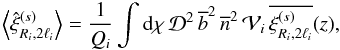 (25)with
  (26)which is the radial
average of the 2ℓi-multipole of
ξ(s), over the 3D spherical shell
associated with the radial bin i in redshift space. Indeed, from the
multipole expansion (11) this also
reads as
(26)which is the radial
average of the 2ℓi-multipole of
ξ(s), over the 3D spherical shell
associated with the radial bin i in redshift space. Indeed, from the
multipole expansion (11) this also
reads as  (27)
(27)
3.2. Comparison with simulations
 |
Fig. 1 Mean redshift-space (solid lines) and real-space (dashed lines) halo correlations,
|
 |
Fig. 2 “2ℓ = 2” redshift-space halo correlation
|
We show in Fig. 1 the mean redshift-space and
real-space halo correlations,  and
and
 ,
over ten distance bins. We find that because of the prefactor
(1 + 2β/3 + β2/5)
in Eq. (12) the monopole redshift-space
correlation is greater than the real-space correlation by 10% for massive halos,
M > 1014 h-1 M⊙,
and by 18% for
M > 2 × 10¹³ h-1 M⊙,
in the redshift range
0 < z < 0.8. The
relative redshift-space distortion is weaker for more massive halos because they have a
larger bias . This
decreases the factor .
,
over ten distance bins. We find that because of the prefactor
(1 + 2β/3 + β2/5)
in Eq. (12) the monopole redshift-space
correlation is greater than the real-space correlation by 10% for massive halos,
M > 1014 h-1 M⊙,
and by 18% for
M > 2 × 10¹³ h-1 M⊙,
in the redshift range
0 < z < 0.8. The
relative redshift-space distortion is weaker for more massive halos because they have a
larger bias . This
decreases the factor .
Although the results from numerical simulations are somewhat noisy, they agree reasonably
well with our analytical predictions. They give the same order of magnitude as our
predictions for both the redshift-space and real-space correlations. In particular, they
fall within the expected 3 − σ error-bars from our analytical predictions
(these error bars are obtained from the analytical covariance matrices derived in
Sect. 4 below). This also shows that the accurate
computation of such quantities remains a difficult task for numerical simulations (in this
case it would require many realizations of the simulated sky resulting in a heavy
computational load) and it is useful to have analytical models for cross-checking. In
particular, while the ratio  is greater than unity and
smooth within the analytical model (it is actually scale-independent in our simple model
(12)), it shows spurious fluctuations in
the simulation data for rare massive halos because of low statistics.
is greater than unity and
smooth within the analytical model (it is actually scale-independent in our simple model
(12)), it shows spurious fluctuations in
the simulation data for rare massive halos because of low statistics.
For practical purposes, Fig. 1 shows that to constrain cosmology with the clustering of X-ray clusters it is necessary to take into account redshift-space distortions if one aims at an accuracy better than 10%.
We show in Fig. 2 our results for the
“2ℓ = 2” redshift-space correlation
 .
This corresponds to the second term of the expansion (11) over Legendre polynomials. As seen from Eq. (13), this term is negative and its amplitude
is larger for more massive halos because of the factor
.
This corresponds to the second term of the expansion (11) over Legendre polynomials. As seen from Eq. (13), this term is negative and its amplitude
is larger for more massive halos because of the factor
 , which grows with the halo bias.
However, because the error bars are much larger for rare massive halos, the associated
signal is more difficult to measure. We obtain a good agreement with the simulations on
large scales but on small scales below 10 h-1 Mpc our model
seems to underestimate the amplitude of this quadrupole component of the redshift-space
correlation. This may be partly due to higher-order contritbutions to Eq. (7) that modify the relationship between
real-space and redshift-space power spectra. For instance, within perturbation theory
next-to-leading terms at order
, which grows with the halo bias.
However, because the error bars are much larger for rare massive halos, the associated
signal is more difficult to measure. We obtain a good agreement with the simulations on
large scales but on small scales below 10 h-1 Mpc our model
seems to underestimate the amplitude of this quadrupole component of the redshift-space
correlation. This may be partly due to higher-order contritbutions to Eq. (7) that modify the relationship between
real-space and redshift-space power spectra. For instance, within perturbation theory
next-to-leading terms at order  arise and
have been found to increase the amplitude of the redshift-space power and to improve the
agreement with simulations (Taruya et al. 2010;
Nishimichi & Taruya 2011). However, we do
not investigate such modifications in this paper.
arise and
have been found to increase the amplitude of the redshift-space power and to improve the
agreement with simulations (Taruya et al. 2010;
Nishimichi & Taruya 2011). However, we do
not investigate such modifications in this paper.
We do not plot the last “2ℓ = 4” term,
 ,
because our analytical computations show that it is very small (smaller than 0.1 on the
scales shown in Figs. 1 and 2) and within the error bars. However, we have checked that our model
agrees with the simulations for
r > 10 h-1 Mpc
(on smaller scales our model again seems to underestimate this correlation).
,
because our analytical computations show that it is very small (smaller than 0.1 on the
scales shown in Figs. 1 and 2) and within the error bars. However, we have checked that our model
agrees with the simulations for
r > 10 h-1 Mpc
(on smaller scales our model again seems to underestimate this correlation).
4. Covariance matrices
4.1. Explicit expressions
We now consider the covariance matrices  of the estimators ,
defined by
of the estimators ,
defined by  (28)To simplify notations, we
do not write the labels Ri and
2ℓi in the covariance matrices and the
subscript i again refers to both the radial bin,
[Ri, −,Ri, +] ,
and the multipole, 2ℓi.
(28)To simplify notations, we
do not write the labels Ri and
2ℓi in the covariance matrices and the
subscript i again refers to both the radial bin,
[Ri, −,Ri, +] ,
and the multipole, 2ℓi.
The results of Valageas et al. (2011) directly
extend to redshift space and we obtain the expression
 (29)with (see also
Landy & Szalay 1993; Szapudi 2001; Bernardeau
et al. 2002a)
(29)with (see also
Landy & Szalay 1993; Szapudi 2001; Bernardeau
et al. 2002a) ![Mathematical equation: \begin{eqnarray} C_{i,j}^{(s)(2)} & = & \delta_{R_i,R_j} \, \frac{2(4\ell_i\!+\!1)(4\ell_j\!+\!1)}{(\Delta\Omega) \QQ_i^2} \int \dd\chi_i \, \cD_i^2 \frac{\dd\vOm_i}{(\Delta\Omega)} \frac{\dd M_i}{M_i} \nonumber \\ && \times \int_i \dd\vs_{i'} \frac{\dd M_{i'}}{M_{i'}} \, \frac{\dd n}{\dd\!\ln M_i} \frac{\dd n}{\dd\!\ln M_{i'}} \nonumber \\ && \times P_{2\ell_i}(\mu_{i'}) P_{2\ell_j}(\mu_{i'}) \left[ 1+\xi^{{\rm h}(s)}_{i,i'} \right] , \label{C2-def}\\ C_{i,j}^{(s)(3)} & \!\! = \! & \frac{4(4\ell_i\!+\!1)(4\ell_j\!+\!1)} {(\Delta\Omega)\QQ_i\QQ_j} \! \int \!\! \dd\chi_i \, \cD_i^2 \frac{\dd\vOm_i} {(\Delta\Omega)} \frac{\dd M_i}{M_i} \int_i \! \dd\vs_{i'} \frac{\dd M_{i'}}{M_{i'}} \nonumber \\ && \times \int_j \dd\vs_{j'} \frac{\dd M_{j'}}{M_{j'}} \; \frac{\dd n}{\dd\!\ln M_i} \frac{\dd n}{\dd\!\ln M_{i'}} \frac{\dd n}{\dd\!\ln M_{j'}} \nonumber \\ && \times P_{2\ell_i}(\mu_{i'}) P_{2\ell_j}(\mu_{j'}) \left[ \xi^{{\rm h}(s)}_{i',j'} + \zeta^{{\rm h}(s)}_{i,i',j'} \right] , \label{C3-def}\\ \!C_{i,j}^{(s)(4)} & \!\! = \! & \frac{(4\ell_i\!+\!1)(4\ell_j\!+\!1)}{\QQ_i\QQ_j} \! \int \! \dd\chi_i \cD_i^2 \frac{\dd\vOm_i}{(\Delta\Omega)} \frac{\dd M_i}{M_i} \int_i \! \dd\vs_{i'} \frac{\dd M_{i'}}{M_{i'}} \nonumber \\ && \times \frac{\dd n}{\dd\!\ln M_i} \frac{\dd n}{\dd\!\ln M_{i'}} \int \! \dd\chi_j \cD_j^2 \frac{\dd\vOm_j}{(\Delta\Omega)} \frac{\dd M_j}{M_j} \int_j \! \dd\vs_{j'} \frac{\dd M_{j'}}{M_{j'}} \nonumber \\ && \times \frac{\dd n}{\dd\!\ln M_j} \frac{\dd n}{\dd\!\ln M_{j'}} P_{2\ell_i}(\mu_{i'}) P_{2\ell_j}(\mu_{j'}) \nonumber \\ && \times \left[ 2 \xi^{{\rm h}(s)}_{i;j'} \xi^{{\rm h}(s)}_{i';j} + \eta^{{\rm h}(s)}_{i,i';j,j'} \right] . \label{C4-def} \end{eqnarray}](/articles/aa/full_html/2012/11/aa19646-12/aa19646-12-eq187.png) Here
we used the same notation as in Valageas et al.
(2011) that we recalled below Eq. (22). Thus, labels i and j refer to objects
that are at the center of the
and
Here
we used the same notation as in Valageas et al.
(2011) that we recalled below Eq. (22). Thus, labels i and j refer to objects
that are at the center of the
and  shells, whereas labels i′ and j′
refer to objects that are within the
and
shells. The pairs { i, i′ } and
{ j, j′ } are located at unrelated
positions in the observational cone, which we integrate over.
shells, whereas labels i′ and j′
refer to objects that are within the
and
shells. The pairs { i, i′ } and
{ j, j′ } are located at unrelated
positions in the observational cone, which we integrate over.
In Eq. (30) we note δRi,Rj the Kronecker symbol with respect to the radial bins. Thus, δRi,Rj is unity if [Ri, −,Ri, +] ≡ [Rj, −,Rj, +] and zero otherwise (we consider non-overlapping radial bins), independently of the multipoles ℓi and ℓj (which may be equal or different). This shot-noise contribution arises from cases where the pairs { i, i′ } and { j, j′ } are the same (i.e., they involve the same two halos), which implies the same pair length.
The label C(n) refers to quantities that involve n distinct objects. Thus, the contributions C(2) and C(3) arise from shot-noise effects (as is apparent through the prefactors 1/(ΔΩ)), associated with the discreteness of the number density distribution, and they would vanish for continuous distributions. However, they also involve the two-point and three-point correlations, and as such they couple discreteness effects with the underlying large-scale correlations of the population. In case of zero large-scale correlations, C(2) remains nonzero because of the unit factor in the brackets and becomes a purely shot-noise contribution, arising solely from discreteness effects. The contribution C(4) is a pure sample-variance contribution and does not depend on the discreteness of the number density distribution (hence there is no 1/(ΔΩ) prefactor).
We can reorganize these various terms into three contributions,  (33)where
 gathers all terms that only depend on the two-point correlation,
 arises from the three-point correlation (i.e., the last term in Eq. (31)), and
 arises from the four-point correlation (i.e., the last term in Eq. (32)). We obtain for the Gaussian contribution
![Mathematical equation: \begin{eqnarray} \label{Cij-G} C_{i,j}^{(s){\rm (G)}} & = & \delta_{R_i,R_j} \frac{2}{(\Delta\Omega)\QQ_i} \left[ \delta_{\ell_i,\ell_j} (4\ell_i+1) + \left\lag\hxi^{(s)}_{R_i;2\ell_i,2\ell_j}\right\rag \right] \nonumber \\ && + \frac{4}{(\Delta\Omega)\QQ_i\QQ_j} \int \dd\chi \, \cD^2 \, \bb^2 \, \nb^3 \, \cV_i \cV_j \, \overline{\xis_{i',j'}} \nonumber \\ && + \frac{2}{\QQ_i\QQ_j} \int \dd\chi \, \cD^5 \, \bb^4 \, \nb^4 \, \cV_i \cV_j \, \overline{\xis_{i;j'} \xis_{i';j}} , \end{eqnarray}](/articles/aa/full_html/2012/11/aa19646-12/aa19646-12-eq206.png) (34)which
involves terms that are constant, linear, and quadratic
over ξ(s). Here we introduced the mean
(34)which
involves terms that are constant, linear, and quadratic
over ξ(s). Here we introduced the mean
 (35)with
 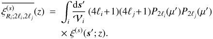 (36)From
the multipole expansion (11) this also
reads as
(36)From
the multipole expansion (11) this also
reads as 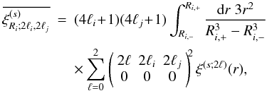 (37)which
involves the square of the Wigner 3-j symbol.
(37)which
involves the square of the Wigner 3-j symbol.
Using the hierarchical ansatz described in Sect. 2.1.3, the contribution
associated with the three-point correlation writes as ![Mathematical equation: \begin{eqnarray} \label{Cij-zeta} C_{i,j}^{(s)(\zeta)} & = & \frac{4}{(\Delta\Omega)\QQ_i\QQ_j} \int \dd\chi \, \cD^2 \, \bb^3 \, \nb^3 \, \cV_i \cV_j \, \frac{S_3}{3} \nonumber \\ && \times \, \left[ \overline{\xis_{i'}} \times \overline{\xis_{j'}} + \overline{\xis_{i',i} \xis_{i',j'}} +\overline{\xis_{j',i} \xis_{j',i'}} \right] , \end{eqnarray}](/articles/aa/full_html/2012/11/aa19646-12/aa19646-12-eq210.png) (38)while
the contribution
associated with the four-point correlation writes as
(38)while
the contribution
associated with the four-point correlation writes as ![Mathematical equation: \begin{eqnarray} \label{Cij-eta} C_{i,j}^{(s)(\eta)} & = & \frac{2}{\QQ_i\QQ_j} \int \dd\chi \, \cD^5 \, \bb^4 \, \nb^4 \, \cV_i \cV_j \, \frac{S_4}{16} \left[ \overline{\xis_{i'}} \times \overline{\xi_{i;j} \xis_{i;j'}} \right . \nonumber \\ && + \overline{\xis_{j'}} \times \overline{\xi_{i;j} \xis_{j;i'}} + 2 \, \overline{\xis_{i'}} \times \overline{\xis_{j'}} \times \xicyl \nonumber \\ && \left. + 2 \overline{\xis_{j';i}\xi_{i;j}\xis_{j;i'}} + \overline{\xis_{j';i}\xis_{i,i'}\xis_{i';j}} + \overline{\xis_{i';j}\xis_{j,j'}\xis_{j';i}} \right] . \end{eqnarray}](/articles/aa/full_html/2012/11/aa19646-12/aa19646-12-eq211.png) (39)Here
the quantities that are overlined are various geometrical averages of the redshift-space
two-point correlation functions. For instance, the geometrical average introduced in the
first integral in Eq. (34) writes as
(39)Here
the quantities that are overlined are various geometrical averages of the redshift-space
two-point correlation functions. For instance, the geometrical average introduced in the
first integral in Eq. (34) writes as
 (40)We
give the explicit expressions of these various terms in Appendix A, and we describe how angular integrations can be performed using the
spherical harmonic decomposition (11), as
well as the flat-sky and Limber’s approximations. All terms involve the redshift-space
correlation ξ(s), except for
(40)We
give the explicit expressions of these various terms in Appendix A, and we describe how angular integrations can be performed using the
spherical harmonic decomposition (11), as
well as the flat-sky and Limber’s approximations. All terms involve the redshift-space
correlation ξ(s), except for
 ,
which only depends on the power along the transverse directions (and is not affected by
redshift-space distortions).
,
which only depends on the power along the transverse directions (and is not affected by
redshift-space distortions).
4.2. Covariance matrix of the monopole redshift-space correlation
In this section we study the covariance matrix
of the monopole redshift-space correlation,  ,
that is,
ℓi = ℓj = 0.
,
that is,
ℓi = ℓj = 0.
4.2.1. Comparison between redshift-space and real-space covariance matrices
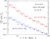 |
Fig. 3 Redshift-space (solid line, for 2ℓ = 0) and real-space (dashed
line) covariance matrices, |
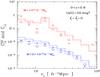 |
Fig. 4 Redshift-space (solid line, for 2ℓ = 0) and real-space (dashed
line) covariance matrices, |
We show in Figs. 3 and 4 the redshift-space and real-space covariance matrices
and
Ci,j, for halos in the redshift range
0 < z < 0.8. The
redshift-space covariance matrix is greater than the real-space covariance matrix by
about 11% along the diagonal and by 20% for off-diagonal entries, for massive halos,
M > 1014 h-1 M⊙.
For
M > 2 × 10¹³ h-1 M⊙,
these amplification factors are higher, 33% along the diagonal and 40% for off-diagonal
entries. This could be expected from the higher value of the redshift-space correlation
function noticed in Fig. 1. This is due to the
amplification of the redshift-space power spectrum through the Kaiser effect, as shown
by Eq. (9). Again, the relative effect is
weaker for rare massive halos because of their larger bias
, which
decreases the associated factor . The
amplification of the covariance matrix is lower along the diagonal, where the covariance
matrix includes a pure shot-noise term (first term in Eq. (34)) that is independent of
ξ(s) and is not amplified by the Kaiser
effect.
We obtain a reasonably good agreement with the numerical simulations for both redshift-space and real-space covariance matrices, for diagonal and off-diagonal entries. The simulation data are somewhat noisier for off diagonal entries and show spurious oscillations in Fig. 4 that are not physical but due to low statistics, especially for rare massive halos. This shows that analytic models are competitive tools to estimate these covariance matrices. In particular, for data analysis purposes it can be helpful to have smooth covariance matrices, which make matrix inversion more reliable.
In any case, redshift-space distortions only have a moderate impact on the covariance matrices and do not change their magnitude. This means that most of the real-space results obtained in Valageas et al. (2011) remain valid.
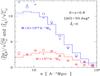 |
Fig. 5 Signal-to-noise ratio of the redshift-space (solid line) and real-space (dashed line) two-point correlations. We show the results obtained for halos in the redshift range 0 < z < 0.8 with an angular window of 50 deg2. |
We show in Fig. 5 an estimate of the
signal-to-noise ratio of the redshift-space and real-space two-point correlations,
defined as  .
A more precise analysis would require using the full covariance matrix, but this ratio
should allow us to check whether redshift distortions, which amplify both the mean
correlation and its covariance matrix, degrade the signal-to-noise ratio. Clearly,
Fig. 5 shows that the signal-to-noise ratio is
not strongly affected by the Kaiser effect. Indeed, the amplification of
.
A more precise analysis would require using the full covariance matrix, but this ratio
should allow us to check whether redshift distortions, which amplify both the mean
correlation and its covariance matrix, degrade the signal-to-noise ratio. Clearly,
Fig. 5 shows that the signal-to-noise ratio is
not strongly affected by the Kaiser effect. Indeed, the amplification of
 overweights the amplification of and
the signal-to-noise ratio slightly increases. This can be understood because the
contributions to that
are cubic over ξ(s) (or of higher order),
which in our framework only come from the four-point correlation contribution (39) to the pure sample-variance term, are
less important than the mixed shot-noise and sample-variance contributions that are
constant or linear over ξ(s).
overweights the amplification of and
the signal-to-noise ratio slightly increases. This can be understood because the
contributions to that
are cubic over ξ(s) (or of higher order),
which in our framework only come from the four-point correlation contribution (39) to the pure sample-variance term, are
less important than the mixed shot-noise and sample-variance contributions that are
constant or linear over ξ(s).
The results found in Fig. 5 mean that redshift distortions do not prevent measuring the clustering of X-ray clusters and its use to constrain cosmology, since the signal-to-noise ratio remains as high and even slightly higher.
4.2.2. Importance of non-Gaussian contributions
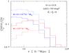 |
Fig. 6 Relative importance of the non-Gaussian contributions
|
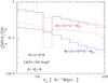 |
Fig. 7 Relative importance of the non-Gaussian contributions
|
We show in Figs. 6 and 7 the ratios  and
and
 .
They give the relative contribution to the covariance matrix of the terms associated
with the three-point correlation function, Eq. (38), or with the four-point correlation function, Eq. (39). For low-mass halos the 4-pt
contribution is
larger than the 3-pt contribution ,
whereas the ordering is reversed for high-mass halos. This agrees with the results
obtained in real-space in Valageas et al. (2011)
(see their Figs. 15 and 16). This behavior is due to the greater importance of
shot-noise effects for rare massive halos. This gives more weight to the 3-pt
contribution, which is part of the coupled shot-noise–sample-variance contribution
C(s)(3) in Eq. (31), than to the 4-pt contribution, which is
part of the pure sample-variance contribution
C(s)(4) in Eq. (32). For the same reason, these non-Gaussian
contributions are relatively smaller along the diagonal for rare halos, as seen on the
fourth bin j = i in Fig. 7.
.
They give the relative contribution to the covariance matrix of the terms associated
with the three-point correlation function, Eq. (38), or with the four-point correlation function, Eq. (39). For low-mass halos the 4-pt
contribution is
larger than the 3-pt contribution ,
whereas the ordering is reversed for high-mass halos. This agrees with the results
obtained in real-space in Valageas et al. (2011)
(see their Figs. 15 and 16). This behavior is due to the greater importance of
shot-noise effects for rare massive halos. This gives more weight to the 3-pt
contribution, which is part of the coupled shot-noise–sample-variance contribution
C(s)(3) in Eq. (31), than to the 4-pt contribution, which is
part of the pure sample-variance contribution
C(s)(4) in Eq. (32). For the same reason, these non-Gaussian
contributions are relatively smaller along the diagonal for rare halos, as seen on the
fourth bin j = i in Fig. 7.
Figures 6 and 7 show that the non-Gaussian contributions can make up to 20−60% of the full covariance matrix as soon as one bin i or j corresponds to scales on the order of 10 h-1 Mpc. Their relative contribution is also somewhat larger for off-diagonal terms. Therefore, although these terms do not change the order of magnitude of the covariance matrix, it is necessary to include them to obtain accurate estimates.
4.2.3. Correlation matrices
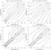 |
Fig. 8 Contour plots for the redshift-space correlation matrices
|


We show in Fig. 8 the redshift-space correlation
matrices defined as  (41)We plot the correlation
matrices associated with the Gaussian part (34) and with the full matrix (33). In agreement with Fig. 7, we can see
that the non-Gaussian contributions, associated with the 3-pt and 4-pt correlations,
make the correlation matrix less diagonal, especially for low-mass halos. As explained
above, this is because rare massive halos show stronger pure shot-noise effects that
give an additional weight to the diagonal entries. In any case, we can see that it is
important to take into account non-Gaussian contributions to obtain accurate estimates.
Moreover, off-diagonal terms cannot be neglected (especially for low-mass halos), hence
it is necessary to use the full covariance matrix
to
draw constraints on cosmology from the analysis of X-ray cluster surveys.
(41)We plot the correlation
matrices associated with the Gaussian part (34) and with the full matrix (33). In agreement with Fig. 7, we can see
that the non-Gaussian contributions, associated with the 3-pt and 4-pt correlations,
make the correlation matrix less diagonal, especially for low-mass halos. As explained
above, this is because rare massive halos show stronger pure shot-noise effects that
give an additional weight to the diagonal entries. In any case, we can see that it is
important to take into account non-Gaussian contributions to obtain accurate estimates.
Moreover, off-diagonal terms cannot be neglected (especially for low-mass halos), hence
it is necessary to use the full covariance matrix
to
draw constraints on cosmology from the analysis of X-ray cluster surveys.
4.3. Covariance matrix of the “ 2 ℓ = 2” redshift-space correlation
We now study the covariance matrix
of the “2ℓ = 2” redshift-space correlation,
,
that is,
2ℓi = 2ℓj = 2.
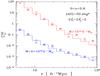 |
Fig. 9 Covariance matrix |
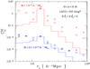 |
Fig. 10 Covariance matrix |
 |
Fig. 11 Relative importance of the non-Gaussian contributions
|
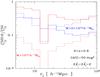 |
Fig. 12 Relative importance of the non-Gaussian contributions
|
We compare in Figs. 9 and 10 our analytical model with numerical simulations for the covariance matrix along the diagonal and along one row. We considered two analyses of the numerical simulations, where we used either 138 nonoverlapping fields separated by a 10 degree gap (squares) or 34 fields separated by a 20 degree gap (crosses). This gives a measure of the statistical error of the simulation data, apart from the systematic finite-resolution effects. Along the diagonal (Fig. 9) our predictions show reasonable agreement with the simulations, which appear reliable with low noise. Along one row (Fig. 10) the simulations give higher off-diagonal entries than our model, but they also show a significant statistical noise. In view of these uncertainties we obtain a reasonable agreement on scales above 10 h-1 Mpc. On smaller scales, our model may underestimate the off-diagonal covariance because of nonlinear effects, as suggested by the comparison for the mean correlation itself shown in Fig. 2. Therefore, on scales above 10 h-1 Mpc analytical models such as the one presented in this paper can provide a competitive alternative to numerical simulations to estimate quantities such as covariance matrices that are difficult to obtain from numerical simulations (as they require large box sizes with a good resolution and time-consuming data analysis procedures).
We show in Figs. 11 and 12 the relative contribution to the covariance matrix of the terms associated with the 3-pt and 4-pt correlation functions. The comparison with Figs. 6 and 7 shows that these non-Gaussian contributions are relatively less important along the diagonal but more important on off-diagonal entries than for the monopole “2ℓ = 0” case. Thus, they make up to 40−60% of the full covariance matrix over a large range of scales.
For completeness we show in Appendix C the
correlation matrices of this “2ℓ = 2” redshift-space correlation, as well
as the cross-correlation between the “2ℓ = 0” and
“2ℓ = 2” components. We find that the “2ℓ = 2”
covariance matrix is significantly more diagonal than the “2ℓ = 0”
covariance matrix and that the cross-correlation matrix between both components is quite
small (~0.05). This means that the full covariance matrix in the
{ Ri,ℓi }
space is approximately block-diagonal (we may neglect entries with
ℓi ≠ ℓj).
Then, we can decouple the analysis of
and .
5. Applications to real survey cases
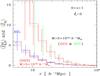 |
Fig. 13 Mean monopole redshift-space (solid lines) and real-space (dashed lines)
correlations, |
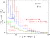 |
Fig. 14 Mean monopole correlations, |
As in Valageas et al. (2011), we now study the correlation functions that can be measured in several cluster surveys. We considered three surveys on limited angular windows:
-
The XXL survey (Pierreet al. 2011) is an XMM Very LargeProgramme specifically designed to constrain the equation ofstate of the dark energy by using clusters of galaxies. It consists oftwo 25 deg2 areas and probes massive clusters out to a redshift of ~2. We considered the “C1 selection function” given in Fig. J.1 of Valageas et al. (2011, see also Pacaud et al. 2006, 2007).
-
The Dark Energy Survey (DES) is an optical imaging survey to cover 5000 deg2 with the Blanco four-meter telescope at the Cerro Tololo Inter-American Observatory2. We considered the expected mass threshold M > 5 × 10¹³ h-1 M⊙, as well as the subset of massive clusters M > 5 × 10¹⁴ h-1 M⊙.
-
The South Pole Telescope (SPT) operates at millimeter wavelengths3. It will cover some 2500 deg2 at three frequencies, aiming at detecting clusters of galaxies from the Sunyaev-Zel’dovich (S-Z) effect. We considered a mass threshold of 5 × 10¹⁴ h-1 M⊙ (Vanderlinde et al. 2010). We also considered three all-sky surveys. In practice, the total angular area of these surveys is not really 4π sterad since we must remove the galactic plane. In the following, for Planck we considered the two-sided cone of angle θs = 75 deg (i.e., |b| > 15 deg), which yields a total area ΔΩ ≃ 30 576 deg2. For Erosita and Euclid we took θs = 59 deg (i.e., |b| > 31 deg), which corresponds to a total area that is about one-half of the full sky, ΔΩ ≃ 20 000 deg2.
-
Planck operates at nine frequencies, enabling an efficient detection of the cluster S-Z signature but has a rather large PSF (5′−10′). Some 1625 massive clusters out to z = 1 are expected over the whole sky. We assumed the selection function by Melin et al. (2006), shown in Fig. J.1 of Valageas et al. (2011).
-
For Erosita, a simple flux limit is currently assumed as an average over the whole sky: 4 × 10-14 erg s-1 cm-2 in the [0.5−2] keV band (Predehl et al. 2009). The associated selection function is shown in Fig. J.1 of Valageas et al. (2011). This would yield 71 907 clusters out to z = 1.
-
For Euclid, we followed the prescription of the Euclid science book for the cluster optical selection function and adopted a fixed mass threshold of 5 × 10¹³ h-1 M⊙ (Refregier et al. 2011).
In the following, the error bars shown in the figures are the statistical error bars associated with the covariance matrices studied in Sect. 4 (i.e., we did not include other sources of uncertainties such as observational noise). For the full-sky surveys this “sample-variance” noise does not vanish because even full-sky surveys up to a given redshift only cover a finite volume. In this limit the “sample variance” is usually called the “cosmic variance”.
5.1. Monopole redshift-space correlation
We show the redshift-space and real-space correlations
and
 that can be measured with these surveys in the redshift range
0 < z < 1 in
Figs. 13 and 14. In each case, the redshift-space correlation is slightly higher than the
real-space correlation. The error bars
that can be measured with these surveys in the redshift range
0 < z < 1 in
Figs. 13 and 14. In each case, the redshift-space correlation is slightly higher than the
real-space correlation. The error bars  correspond to the diagonal entries of the redshift-space covariance matrix.
Redshift-space distortions can be seen in these figures, but in several cases they are
smaller than the error bars. To see the impact of these redshift-space distortions more
clearly, we show the ratio 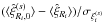 in Figs. 15 and 16. This gives the difference between the monopole redshift-space and real-space
correlations in units of the standard deviation
in Figs. 15 and 16. This gives the difference between the monopole redshift-space and real-space
correlations in units of the standard deviation  ,
that is, of the error bar of the measure.
,
that is, of the error bar of the measure.
Among limited-area surveys, the amplification of the cluster correlation function by the
Kaiser effect will be clearly seen for halos above
M > 5 × 10¹³ h-1 M⊙
in DES. The effect is negligible for more massive halos,
M > 5 × 10¹⁴ h-1 M⊙,
in DES and SPT, because of their larger error bars (see Fig. 13). For the “C1 clusters” measured in the XXL survey redshift
distortions are marginally relevant: they are on the order of
 in distance bins around 15 h-1 Mpc, so that by collecting
the signal from all distance bins they would give a signal-to-noise ratio of about unity.
in distance bins around 15 h-1 Mpc, so that by collecting
the signal from all distance bins they would give a signal-to-noise ratio of about unity.
Among full-sky surveys, the redshift-space amplification will have a clear impact for the full cluster populations measured in Erosita and Euclid, and a marginal impact for Planck. Again, subsamples of massive clusters, M > 5 × 10¹⁴ h-1 M⊙, lead to large error bars that hide this redshift-space effect.
In practice one does not measure both real-space and redshift-space correlations from a
cluster survey, because one does not have a map of the cluster velocities. Therefore, the
redshift-space amplification of the spherically averaged correlation
is
degenerate with the halo bias (which is
difficult to predict with a high accuracy). To measure redshift-space distortions, one
needs to measure the anisotropies of the redshift-space correlation, that is, the
higher-order multipoles ξ(s;2) and
ξ(s;4) of Eq. (11). This provides a distinctive signature
that breaks the degeneracy with the halo bias and yields another constraint on cosmology
through the factor β, that is, the growth rate f of the
density fluctuations defined in Eq. (8). We
consider these higher-order multipoles in the following sections.
5.2. “2 ℓ = 2” redshift-space correlation
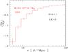 |
Fig. 17 Mean “2ℓ = 2” redshift-space correlation
|
We show in Figs. 17 and 18 the mean “2ℓ = 2” redshift-space correlation
 . We
considered the same surveys as in Sect. 5.1, but we
only plot our results for the cases where the signal-to-noise ratio is higher than unity.
In agreement with the analysis of Sect. 3, this
quadrupole term is more difficult to measure than the monopole term studied in Sect. 5.1, and only DES, Erosita, and Euclid can obtain a
clear detection. Even for these surveys, the correlation can only be measured for the full
halo population and error bars become too large if one restricts to the subsample of rare
massive halos above
5 × 10¹⁴ h-1 M⊙.
Nevertheless, it will be useful to measure this “2ℓ = 2” redshift-space
correlation in these surveys because this should tighten the constraints on cosmology.
Indeed, a simultaneous analysis of and
constrains the factor , and in turn
the halo bias and the growth rate of density fluctuations.
. We
considered the same surveys as in Sect. 5.1, but we
only plot our results for the cases where the signal-to-noise ratio is higher than unity.
In agreement with the analysis of Sect. 3, this
quadrupole term is more difficult to measure than the monopole term studied in Sect. 5.1, and only DES, Erosita, and Euclid can obtain a
clear detection. Even for these surveys, the correlation can only be measured for the full
halo population and error bars become too large if one restricts to the subsample of rare
massive halos above
5 × 10¹⁴ h-1 M⊙.
Nevertheless, it will be useful to measure this “2ℓ = 2” redshift-space
correlation in these surveys because this should tighten the constraints on cosmology.
Indeed, a simultaneous analysis of and
constrains the factor , and in turn
the halo bias and the growth rate of density fluctuations.
5.3. “2 ℓ = 4” redshift-space correlation
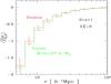 |
Fig. 18 Mean “2ℓ = 2” redshift-space correlation
|
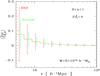 |
Fig. 19 Mean “2ℓ = 4”redshift-space correlation
|
We show in Fig. 19 the mean
“2ℓ = 4” redshift-space correlation
 . The
signal is even weaker than for the “2ℓ = 2” correlation and only DES and
Euclid may be able to obtain a detection. DES is unlikely to provide an accurate measure
but it should still give useful upper bounds. Euclid may obtain a significant measure of
the overall amplitude by gathering the information from all distance bins. This would
provide an additional constraint on β to the one provided by the mutipole
“2ℓ = 2” of Fig. 18.
. The
signal is even weaker than for the “2ℓ = 2” correlation and only DES and
Euclid may be able to obtain a detection. DES is unlikely to provide an accurate measure
but it should still give useful upper bounds. Euclid may obtain a significant measure of
the overall amplitude by gathering the information from all distance bins. This would
provide an additional constraint on β to the one provided by the mutipole
“2ℓ = 2” of Fig. 18.
6. Conclusion
We have generalized our previous study of the real-space correlation functions of clusters of galaxies (Valageas et al. 2011) to include redshift-space distortions. On large scales they lead to an anisotropic correlation function because of the Kaiser effect, due to the correlation between density and velocity fields. There are no “fingers of God” because clusters are the largest bound objects, as opposed to galaxies that can have performed several orbital revolutions within a larger halo and show a high small-scale velocity dispersion. Then, taking into account this Kaiser effect at leading order and using a simple hierarchical model for the three-point and four-point halo correlations, we developed an analytical formalism to obtain explicit expressions for the mean redshift-space correlations and their covariance matrices. We included shot-noise and sample-variance effects as well as Gaussian and non-Gaussian contributions. This is a direct extension of the formalism presented in Valageas et al. (2011) for real-space correlations.
Expanding as usual the angular anisotropy of the redshift-space correlation on Legendre polynomials, we considered the first three nonzero multipoles: the monopole 2ℓ = 0 (i.e. the spherically-averaged correlation), the quadrupole, 2ℓ = 2, and the next multipole, 2ℓ = 4. Higher-order multipoles should arise from nonlinear corrections to the Kaiser effect. Although they are not studied here, which would require a more complex nonlinear modeling of the Kaiser effect itself, their analysis could be performed using the formalism developped in this paper (one only needs to include higher multipoles in the sums that appear in the expressions of the covariance matrices). However, for practical purposes they are probably irrelevant for clusters of galaxies. Indeed, higher-order multipoles are increasingly difficult to measure and we found that the third mutipole, 2ℓ = 4, may only be detected (at a 1 − σ level) by Euclid or a similar survey.
We obtained a reasonable agreement with numerical simulations for the mean correlations and covariance matrices on large scales (r > 10 h-1 Mpc). Redshift-space distortions amplify the monopole correlation by about 10−20%, depending on the halo mass. The covariance matrix is also amplified by 10−40% and the signal-to-noise ratio remains of the same order as for the real-space correlation. We found that non-Gaussian terms can contribute to the covariance matrices up to 20−60%, especially for nondiagonal entries when one of the two bins corresponds to small scales (~10 h-1 Mpc). They make the correlation matrices less diagonal. We also found that the correlation matrices of the quadrupole (2ℓ = 2) are significantly more diagonal than the correlation matrices of the monopole (2ℓ = 0). On the other hand, the cross-correlations of the monopole and quadrupole are quite small, on the order of 0.05. This means that the full covariance matrix is approximately block-diagonal in the space { Ri,2ℓi } , that is, we may decouple the analysis of the monopole and quadrupole.
Our predictions for ongoing and future surveys (only taking into account the
sample-variance and shot-noise contributions) show that the impact of redshift distortions
on the spherical-averaged correlation (i.e. the monopole) will only be significant for DES,
Erosita, and Euclid. For the other surveys investigated here, XXL, SPT, and
Planck, the difference  , between
the redshift-space and real-space correlations, falls below “1 − σ” of the
statistical error bar. In practice, even for these surveys it would be better to compare the
data with theoretical predictions for the redshift-space correlations rather than the
real-space correlations, since simple models for the latter are not more difficult to
implement and one does not need a very accurate modeling of redshift distortions. For
covariance matrices, it is sufficient to use the real-space ones, which are easier to
compute. For DES, Erosita, and Euclid, one should take into account redshift-space
distortions for both the mean correlations and their covariance matrices. However, because
of their modest impact on the covariance matrices (see Figs. 3 and 4) and the limited accuracy of such
computations, it is probably sufficient to use the real-space covariance matrices in a first
step.
, between
the redshift-space and real-space correlations, falls below “1 − σ” of the
statistical error bar. In practice, even for these surveys it would be better to compare the
data with theoretical predictions for the redshift-space correlations rather than the
real-space correlations, since simple models for the latter are not more difficult to
implement and one does not need a very accurate modeling of redshift distortions. For
covariance matrices, it is sufficient to use the real-space ones, which are easier to
compute. For DES, Erosita, and Euclid, one should take into account redshift-space
distortions for both the mean correlations and their covariance matrices. However, because
of their modest impact on the covariance matrices (see Figs. 3 and 4) and the limited accuracy of such
computations, it is probably sufficient to use the real-space covariance matrices in a first
step.
The quadrupole, 2ℓ = 2, is more difficult to measure from the distribution of clusters of galaxies, and we found that only DES, Erosita, and Euclid, among the surveys considered here, will likely provide a useful measure. In this respect, clusters are less efficient than galaxies in measuring redshift-space distortions. Even though clusters have a higher bias and stronger correlations, they are much less numerous than galaxies. This leads to a lower signal-to-noise ratio for the quadrupole. Nevertheless, such a measure would provide a nice supplement and would help tighten the constraints on cosmology. An extension of this paper would be to study on a quantitative level the expected improvement brought by this measure for these surveys. This requires a statistical analysis, using Fisher matrices or likelihood functions, which we leave for future works.
The last multipole generated at linear order by the Kaiser effect, 2ℓ = 4, is very difficult to measure from cluster surveys and we found that only Euclid will likely be able to provide a meaningful measure. Nonlinear corrections will generate higher-order multipoles but they are likely to be even more difficult to measure. Therefore, for practical purposes redshift-space distortions should only impact cluster correlations at the level of the monopole and quadrupole components.
Our results deliberately disregard observational constraints related to cluster redshifts estimation. In practice, measuring cluster redshifts is a costly task that consists in obtaining spectra for a few (> 10) galaxies pertaining to each cluster, leading to errors on the order of σ(z) < 0.01(1 + z). This precision depends on the number of measured spectra, which in turn depends on cluster richness (and consequently, on its mass), cluster apparent size, morphological complexity, dynamical state, and distance to the observer, as well as on fixed instrumental constraints. In some cases, only the brightest central galaxy (BCG) can have its redshift measured. This may result in a biased cluster redshift estimate, for the BCG may have a small proper motion within the cluster potential well (Adami & Ulmer 2000; Oegerle & Hill 2001; Coziol et al. 2009). In many other cases, only photometric redshifts will be obtained, resulting in larger redshift uncertainties – on the order of σ(z) ~ 0.05(1 + z) (e.g. Pillepich et al. 2012). However, recent studies have underlined the potential of photometric surveys for studying redshift space distortions at the galaxy scale, using the information in the (2D) angular correlation function (e.g. Ross et al. 2011). We leave the application of this method to clusters to future work, and note that a quantitative analysis (e.g. a Fisher analysis) would largely benefit from a proper modeling of follow-up incompleteness, uncertainties, and biases on cluster redshifts given the halo masses and positions.
We can neglect the impact of the change from x to
s on background cosmological quantities such as the
radial and angular distances χ
and  ,
which vary on scales on the order of
c/H0. Redshift-space
distortions only have a significant effect on the correlation
ξ(s) of the halo population, which is
studied on smaller scales ~20 h-1 Mpc and becomes
anisotropic.
,
which vary on scales on the order of
c/H0. Redshift-space
distortions only have a significant effect on the correlation
ξ(s) of the halo population, which is
studied on smaller scales ~20 h-1 Mpc and becomes
anisotropic.
Acknowledgments
We thank M. Pierre and C. Adami for useful discussions. We thank R. Teyssier for providing us with the halo catalog from the “horizon” simulation. This work was performed using HPC resources from GENCI-CCRT (Grant 2012-t2012046803).
References
- Abell, G. O. 1958, ApJS, 3, 211 [NASA ADS] [CrossRef] [Google Scholar]
- Adami, C., & Ulmer, M. P. 2000, A&A, 361, 13 [NASA ADS] [Google Scholar]
- Benjamin, J., Heymans, C., Semboloni, E., et al. 2007, MNRAS, 381, 702 [NASA ADS] [CrossRef] [Google Scholar]
- Bernardeau, F., Colombi, S., Gaztañaga, E., & Scoccimarro, R. 2002a, Phys. Rep., 367, 1 [NASA ADS] [CrossRef] [EDP Sciences] [MathSciNet] [Google Scholar]
- Bernardeau, F., Mellier, Y., & van Waerbeke, L. 2002b, A&A, 389, L28 [Google Scholar]
- Bernstein, G. M. 1994, ApJ, 424, 569 [NASA ADS] [CrossRef] [Google Scholar]
- Blake, C., Davis, T., Poole, G. B., et al. 2011a, MNRAS, 415, 2892 [NASA ADS] [CrossRef] [Google Scholar]
- Blake, C., Glazebrook, K., Davis, T. M., et al. 2011b, MNRAS, 418, 1725 [NASA ADS] [CrossRef] [Google Scholar]
- Böhringer, H., Schuecker, P., Guzzo, L., et al. 2001, A&A, 369, 826 [NASA ADS] [CrossRef] [EDP Sciences] [Google Scholar]
- Borgani, S., Rosati, P., Tozzi, P., et al. 2001, ApJ, 561, 13 [NASA ADS] [CrossRef] [Google Scholar]
- Burenin, R. A., Vikhlinin, A., Hornstrup, A., et al. 2007, ApJS, 172, 561 [NASA ADS] [CrossRef] [Google Scholar]
- Cabré, A., & Gaztañaga, E. 2009, MNRAS, 396, 1119 [NASA ADS] [CrossRef] [Google Scholar]
- Clerc, N., Sadibekova, T., Pierre, M., et al. 2012, MNRAS, in press [Google Scholar]
- Cole, S., Percival, W. J., Peacock, J. A., et al. 2005, MNRAS, 362, 505 [NASA ADS] [CrossRef] [Google Scholar]
- Colombi, S., Dodelson, S., & Widrow, L. M. 1996, ApJ, 458, 1 [NASA ADS] [CrossRef] [Google Scholar]
- Coziol, R., Andernach, H., Caretta, C. A., Alamo-Martínez, K. A., & Tago, E. 2009, AJ, 137, 4795 [NASA ADS] [CrossRef] [Google Scholar]
- Desjacques, V., Crocce, M., Scoccimarro, R., & Sheth, R. K. 2010, Phys. Rev. D, 82, 103529 [NASA ADS] [CrossRef] [Google Scholar]
- Eisenstein, D. J., & Hut, P. 1998, ApJ, 498, 137 [NASA ADS] [CrossRef] [Google Scholar]
- Eisenstein, D. J., Weinberg, D. H., Agol, E., et al. 2011, AJ, 142, 72 [Google Scholar]
- Eisenstein, D. J., Zehavi, I., Hogg, D. W., et al. 2005, ApJ, 633, 560 [NASA ADS] [CrossRef] [Google Scholar]
- Fry, J. N. 1984, ApJ, 277, L5 [NASA ADS] [CrossRef] [Google Scholar]
- Gradshteyn, I. S., & Ryzhik, I. M. 1994, Table of integrals, series and products, eds. I. S. Gradshteyn, & I. M. Ryzhik (New York: Academic Press) [Google Scholar]
- Groth, E. J., & Peebles, P. J. E. 1977, AJ, 217, 385 [NASA ADS] [CrossRef] [Google Scholar]
- Guzzo, L., Pierleoni, M., Meneux, B., et al. 2008, Nature, 451, 541 [NASA ADS] [CrossRef] [PubMed] [Google Scholar]
- Hamilton, A. J. S. 1992, ApJ, 385, L5 [NASA ADS] [CrossRef] [Google Scholar]
- Jackson, J. C. 1972, MNRAS, 156, 1P [Google Scholar]
- Kaiser, N. 1987, MNRAS, 227, 1 [NASA ADS] [CrossRef] [Google Scholar]
- Kaiser, N. 1992, ApJ, 388, 272 [NASA ADS] [CrossRef] [Google Scholar]
- Katgert, P., Mazure, A., Perea, J., et al. 1996, A&A, 310, 8 [NASA ADS] [Google Scholar]
- Kilbinger, M., Benabed, K., Guy, J., et al. 2009, A&A, 497, 677 [NASA ADS] [CrossRef] [EDP Sciences] [Google Scholar]
- Koester, B. P., McKay, T. A., Annis, J., et al. 2007a, ApJ, 660, 239 [NASA ADS] [CrossRef] [Google Scholar]
- Koester, B. P., McKay, T. A., Annis, J., et al. 2007b, ApJ, 660, 221 [NASA ADS] [CrossRef] [Google Scholar]
- Komatsu, E., Smith, K. M., Dunkley, J., et al. 2011, ApJS, 192, 18 [NASA ADS] [CrossRef] [Google Scholar]
- Landy, S. D., & Szalay, A. S. 1993, ApJ, 412, 64 [NASA ADS] [CrossRef] [Google Scholar]
- Limber, D. N. 1953, ApJ, 117, 134 [NASA ADS] [CrossRef] [Google Scholar]
- Manera, M., & Gaztanaga, E. 2011, MNRAS, 415, 383 [NASA ADS] [CrossRef] [Google Scholar]
- Mantz, A., Allen, S. W., Rapetti, D., & Ebeling, H. 2010, MNRAS, 406, 1759 [NASA ADS] [Google Scholar]
- Massey, R., Rhodes, J., Leauthaud, A., et al. 2007, ApJS, 172, 239 [NASA ADS] [CrossRef] [MathSciNet] [Google Scholar]
- Mehrtens, N., Romer, A. K., Lloyd-Davies, E. J., et al. 2012, MNRAS, 423, 1024 [NASA ADS] [CrossRef] [Google Scholar]
- Meiksin, A., & White, M. 1999, MNRAS, 308, 1179 [NASA ADS] [CrossRef] [Google Scholar]
- Melin, J.-B., Bartlett, J. G., & Delabrouille, J. 2006, A&A, 459, 341 [NASA ADS] [CrossRef] [EDP Sciences] [Google Scholar]
- Moles, M., Benítez, N., Aguerri, J. A. L., et al. 2008, AJ, 136, 1325 [Google Scholar]
- Munshi, D., Valageas, P., van Waerbeke, L., & Heavens, A. 2008, Phys. Rep., 462, 67 [NASA ADS] [CrossRef] [Google Scholar]
- Nishimichi, T., & Taruya, A. 2011, Phys. Rev. D, 84, 043526 [NASA ADS] [CrossRef] [Google Scholar]
- Oegerle, W. R., & Hill, J. M. 2001, AJ, 122, 2858 [NASA ADS] [CrossRef] [Google Scholar]
- Pacaud, F., Pierre, M., Adami, C., et al. 2007, MNRAS, 382, 1289 [NASA ADS] [CrossRef] [Google Scholar]
- Pacaud, F., Pierre, M., Refregier, A., et al. 2006, MNRAS, 372, 578 [NASA ADS] [CrossRef] [Google Scholar]
- Peacock, J. A., Cole, S., Norberg, P., et al. 2001, Nature, 410, 169 [NASA ADS] [CrossRef] [PubMed] [Google Scholar]
- Peebles, P. J. E. 1980, The large-scale structure of the universe, ed. P. J. E. Peebles, (Princeton, N.J., USA:Princeton University Press) [Google Scholar]
- Peebles, P. J. E., & Hauser, M. G. 1974, ApJS, 28, 19 [NASA ADS] [CrossRef] [Google Scholar]
- Percival, W. J., & White, M. 2009, MNRAS, 393, 297 [NASA ADS] [CrossRef] [Google Scholar]
- Pierre, M., Pacaud, F., Juin, J. B., et al. 2011, MNRAS, 414, 1732 [NASA ADS] [CrossRef] [Google Scholar]
- Pillepich, A., Porciani, C., & Reiprich, T. H. 2012, MNRAS, 422, 44 [NASA ADS] [CrossRef] [Google Scholar]
- Planck Collaboration 2011, A&A, 536, A8 [NASA ADS] [CrossRef] [EDP Sciences] [Google Scholar]
- Predehl, P., Boehringer, H., & et al., H. B. 2009, Proc. Conf. X-ray Astronomy 2009, Bologna, September 2009 [Google Scholar]
- Refregier, A., Amara, A., Kitching, T. D., & Rassat, A. 2011, A&A, 528, A33 [NASA ADS] [CrossRef] [EDP Sciences] [Google Scholar]
- Reichardt, C. L., Stalder, B., Bleem, L. E., et al. 2012, ApJ, submitted [arXiv:1203.5775] [Google Scholar]
- Reid, B. A., & White, M. 2011, MNRAS, 417, 1913 [NASA ADS] [CrossRef] [Google Scholar]
- Reid, B. A., Samushia, L., White, M., et al. 2012, MNRAS, submitted [arXiv:1203.6641] [Google Scholar]
- Ross, N. P., da Ângela, J., Shanks, T., et al. 2007, MNRAS, 381, 573 [NASA ADS] [CrossRef] [Google Scholar]
- Ross, A. J., Percival, W. J., Crocce, M., Cabré, A., & Gaztañaga, E. 2011, MNRAS, 415, 2193 [NASA ADS] [CrossRef] [Google Scholar]
- Rozo, E., Wechsler, R. H., Rykoff, E. S., et al. 2010, ApJ, 708, 645 [NASA ADS] [CrossRef] [Google Scholar]
- Sarazin, C. L. 1988, X-ray emission from clusters of galaxies [Google Scholar]
- Schrabback, T., Hartlap, J., Joachimi, B., et al. 2010, A&A, 516, A63 [NASA ADS] [CrossRef] [EDP Sciences] [Google Scholar]
- Sehgal, N., Trac, H., Acquaviva, V., et al. 2011, ApJ, 732, 44 [NASA ADS] [CrossRef] [Google Scholar]
- Slosar, A., Font-Ribera, A., Pieri, M. M., et al. 2011, J. Cosmology Astropart. Phys., 9, 1 [Google Scholar]
- Smith, R. E., Peacock, J. A., Jenkins, A., et al. 2003, MNRAS, 341, 1311 [NASA ADS] [CrossRef] [Google Scholar]
- Spergel, D. N., Bean, R., Doré, O., et al. 2007, ApJS, 170, 377 [NASA ADS] [CrossRef] [Google Scholar]
- Sunyaev, R. A., & Zeldovich, Y. B. 1972, Comments on Astrophysics and Space Physics, 4, 173 [Google Scholar]
- Szapudi, I. 2001, in Annals of the New York Academy of Sciences, The Onset of Nonlinearity in Cosmology, ed. J. N. Fry, J. R. Buchler, & H. Kandrup, 927, 94 [Google Scholar]
- Szapudi, I., & Colombi, S. 1996, ApJ, 470, 131 [NASA ADS] [CrossRef] [Google Scholar]
- Taruya, A., Nishimichi, T., & Saito, S. 2010, Phys. Rev. D, 82, 063522 [NASA ADS] [CrossRef] [Google Scholar]
- Teyssier, R. 2002, A&A, 385, 337 [NASA ADS] [CrossRef] [EDP Sciences] [Google Scholar]
- Teyssier, R., Pires, S., Prunet, S., et al. 2009, A&A, 497, 335 [NASA ADS] [CrossRef] [EDP Sciences] [Google Scholar]
- Tinker, J., Kravtsov, A. V., Klypin, A., et al. 2008, ApJ, 688, 709 [NASA ADS] [CrossRef] [Google Scholar]
- Tinker, J. L., Robertson, B. E., Kravtsov, A. V., et al. 2010, ApJ, 724, 878 [NASA ADS] [CrossRef] [Google Scholar]
- Valageas, P., Clerc, N., Pacaud, F., & Pierre, M. 2011, A&A, 536, A95 [NASA ADS] [CrossRef] [EDP Sciences] [Google Scholar]
- Vanderlinde, K., Crawford, T. M., de Haan, T., et al. 2010, ApJ, 722, 1180 [NASA ADS] [CrossRef] [Google Scholar]
Appendix A: Computation of geometrical averages
We give in this appendix the explicit expressions of the various geometrical averages of
two-point correlations that are needed to compute the covariance matrix
,
within our framework. We followed the method and the notations of Valageas et al. (2011) while we extend their results to redshift-space
(especially their Appendix F).
The second term in Eq. (34) involves the
average (40) of the correlation between
two concentric spherical shells. Defining the 3D Fourier transform of the
2ℓ-multipole top-hat as  (A.1)where again
μr = (ez·r)/r,
the 3D Fourier-space window of the i-shell reads as
(A.1)where again
μr = (ez·r)/r,
the 3D Fourier-space window of the i-shell reads as  (A.2)In
Eq. (A.1) the subscript 3 recalls that
we consider a 3D window. To simplify notations we did not recall this fact in the window
(A.2)In
Eq. (A.1) the subscript 3 recalls that
we consider a 3D window. To simplify notations we did not recall this fact in the window
 associated with each 3D radial bin. In studies of the real-space correlation (Valageas et al. 2011), only the usual top-hat window
 appears, which does not depend
on the angle of k. Here, because we study the anisotropic
redshift-space correlation and its various multipoles (25) higher-order multipoles
appears, which does not depend
on the angle of k. Here, because we study the anisotropic
redshift-space correlation and its various multipoles (25) higher-order multipoles  appear,
which depend on the direction of k. Equation (A.1) also reads as
appear,
which depend on the direction of k. Equation (A.1) also reads as
 (A.3)where the angular
dependence has been factored out, with
(A.3)where the angular
dependence has been factored out, with 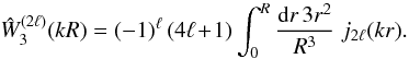 (A.4)This yields for the
window of the i-shell,
(A.4)This yields for the
window of the i-shell,
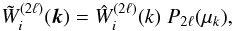 (A.5)with
 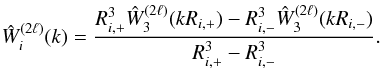 (A.6)In
practice, the redshift-space correlation of clusters of galaxies should be dominated by
the Kaiser effect and the lower multipoles 2ℓ = 0,2, and
4 as in Eqs. (11)−(14). Therefore, we only give explicit
expressions for low-order multipoles, which read as
(A.6)In
practice, the redshift-space correlation of clusters of galaxies should be dominated by
the Kaiser effect and the lower multipoles 2ℓ = 0,2, and
4 as in Eqs. (11)−(14). Therefore, we only give explicit
expressions for low-order multipoles, which read as ![Mathematical equation: \appendix \setcounter{section}{1} \begin{eqnarray} \label{W3-0} \hW_3^{(0)}(k R) &=& 3 \, \frac{\sin(kR)-kR\cos(kR)}{(kR)^3} , \\ \label{W3-2} \hW_3^{(2)}(k R) & = & \frac{-15}{(kR)^3} \left[ kR\cos(kR) - 4 \sin(kR) + 3 \, {\rm Si}(kR) \right] , \nonumber \\ \\ \hW_3^{(4)}(k R) & = & \frac{27}{2(kR)^5} \left[ (105 \!-\! 2(kR)^2) kR\cos(kR) \right. \nonumber \\ \label{W3-4} && \left. - (105 \!-\! 22(kR)^2) \sin(kR) + 15 (kR)^2 \, {\rm Si}(kR) \right] , \end{eqnarray}](/articles/aa/full_html/2012/11/aa19646-12/aa19646-12-eq307.png) where
where
 is the sine integral. Then,
writing the two-point correlation function in Eq. (40) in terms of the power spectrum (9), the angular integration gives
is the sine integral. Then,
writing the two-point correlation function in Eq. (40) in terms of the power spectrum (9), the angular integration gives 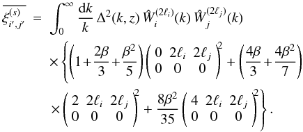 (A.10)Next,
the last term in Eq. (34) involves the
non-connected four-point average
(A.10)Next,
the last term in Eq. (34) involves the
non-connected four-point average 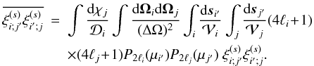 (A.11)As
in Valageas et al. (2011), expressing the two-point
correlation functions in terms of the power spectrum, using the flat-sky (small angle)
approximation, as well as Limber’s approximation (Limber
1953; Kaiser 1992; Munshi et al. 2008), we obtain
(A.11)As
in Valageas et al. (2011), expressing the two-point
correlation functions in terms of the power spectrum, using the flat-sky (small angle)
approximation, as well as Limber’s approximation (Limber
1953; Kaiser 1992; Munshi et al. 2008), we obtain 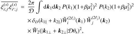 (A.12)where
μi = (ez·ki)/ki,
θs is the angular radius of the survey window (in the
flat-sky approximation),
(A.12)where
μi = (ez·ki)/ki,
θs is the angular radius of the survey window (in the
flat-sky approximation), 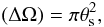 (A.13)and
 is the 2D Fourier-space circular window,
  (A.14)Introducing an auxiliary
wavenumber k⊥ with a Dirac factor
∫dk⊥δD(k⊥ − k1⊥ − k2⊥)
and using the exponential representation of Dirac functions, we can partially factorize
the integrals and perform a few angular integrations. This yields
(A.14)Introducing an auxiliary
wavenumber k⊥ with a Dirac factor
∫dk⊥δD(k⊥ − k1⊥ − k2⊥)
and using the exponential representation of Dirac functions, we can partially factorize
the integrals and perform a few angular integrations. This yields  (A.15)where we introduced
 (A.16)and
 (A.17)Using the multipole
decomposition (11) and the expansion of
plane waves on spherical harmonics, we can write
(A.17)Using the multipole
decomposition (11) and the expansion of
plane waves on spherical harmonics, we can write  as
as  (A.18)where the sum over
ℓ runs up to 4 because the expansion (11) only includes the terms 0 ≤ ℓ ≤ 2 and we only
study estimators
with 0 ≤ ℓi ≤ 2. If we consider a model where
the redshift-space correlation includes multipoles up to 2ℓmax
and we study estimators up to order
(A.18)where the sum over
ℓ runs up to 4 because the expansion (11) only includes the terms 0 ≤ ℓ ≤ 2 and we only
study estimators
with 0 ≤ ℓi ≤ 2. If we consider a model where
the redshift-space correlation includes multipoles up to 2ℓmax
and we study estimators up to order  the sum (A.18) runs up to
 .
Here we introduced
.
Here we introduced ![Mathematical equation: \appendix \setcounter{section}{1} \begin{eqnarray} \label{cI-3-W3} \cI_{i,2\ell_i}^{(s;2\ell)}(r) & = & (4\ell \!+\! 1) \sum_{\ell'=0}^2 \int_0^{\infty} \frac{\dd x \; x \, \xi^{(s;2\ell')}(x)} {r(\Rip^3-\Rim^3)} \nonumber \\ && \times \left[ \Rip^2 \cW_{\ell_i}^{(\ell,\ell')}\! \left(\frac{r}{\Rip},\frac{x}{\Rip}\right) \right. \nonumber \\ && \left. - \Rim^2 \cW_{\ell_i}^{(\ell,\ell')} \! \left(\frac{r}{\Rim},\frac{x}{\Rim}\right) \right] , \end{eqnarray}](/articles/aa/full_html/2012/11/aa19646-12/aa19646-12-eq329.png) (A.19)and
(A.19)and
 (A.20)Then,
substituting the expansion (A.18) into
Eq. (A.15) we obtain
(A.20)Then,
substituting the expansion (A.18) into
Eq. (A.15) we obtain  (A.21)with
 (A.22)where we used that
A(s) defined in Eq. (A.16) also writes as
(A.22)where we used that
A(s) defined in Eq. (A.16) also writes as 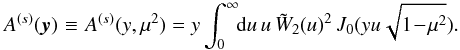 (A.23)These
expressions closely follow those obtained in Valageas
et al. (2011). To recover their real-space results, it is sufficient to set
β = 0 in Eq. (9), which
makes the power spectrum isotropic so that only monopole contributions (i.e.,
ℓ = 0) remain. Thus, in Eq. (A.21) there only remains the term
ℓ = ℓ′ = 0, and the function
A(0,0)(y) can actually be
computed explicitly (see their Eqs. (F10) and (F11)).
(A.23)These
expressions closely follow those obtained in Valageas
et al. (2011). To recover their real-space results, it is sufficient to set
β = 0 in Eq. (9), which
makes the power spectrum isotropic so that only monopole contributions (i.e.,
ℓ = 0) remain. Thus, in Eq. (A.21) there only remains the term
ℓ = ℓ′ = 0, and the function
A(0,0)(y) can actually be
computed explicitly (see their Eqs. (F10) and (F11)).
As in Valageas et al. (2011), we preferred to use
the configuration-space expression (A.21)
rather than the Fourier-space expression (A.12) for numerical computations. Indeed, the integrals have been partially
factored out in Eq. (A.21) (so that it has
the same level of complexity as a two-dimensional integral) and the oscillatory kernels
 of Eq. (A.12) have been replaced by the
slowly-varying kernels
of Eq. (A.12) have been replaced by the
slowly-varying kernels  of Eq. (A.19), see Eqs. (B.17)−(B.19).
We now turn to the contribution (38) that
arises from the three-point correlation function. The first term within the brackets in
Eq. (38) involves the product of two
averages  and
and  ,
which are given in Eq. (27). Following the analysis of Valageas et al. (2011), the second term can be written
in configuration space as
,
which are given in Eq. (27). Following the analysis of Valageas et al. (2011), the second term can be written
in configuration space as 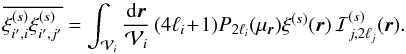 (A.24)Using the expansions
(11) and (A.18), this yields
(A.24)Using the expansions
(11) and (A.18), this yields  (A.25)The
third term within the brackets in Eq. (38)
is obtained from Eq. (A.25) by exchanging
the labels “i” and “j”.
(A.25)The
third term within the brackets in Eq. (38)
is obtained from Eq. (A.25) by exchanging
the labels “i” and “j”.
We now turn to the contribution (39) that
arises from the four-point correlation function, proceeding in a similar fashion. The new
geometrical average involved by the first two terms within the brackets in Eq. (39) reads as  (A.26)which
does not depend on the bin i. The third term involves the cylindrical
average
(A.26)which
does not depend on the bin i. The third term involves the cylindrical
average 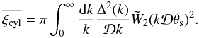 (A.27)The fourth term,
which does not factor, gives rise to
(A.27)The fourth term,
which does not factor, gives rise to 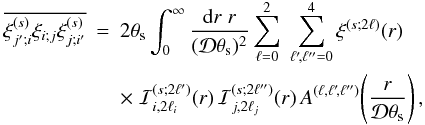 (A.28)where
we introduced, as in Eq. (A.22),
(A.28)where
we introduced, as in Eq. (A.22),
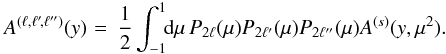 (A.29)The
last two terms within the brackets in Eq. (39) involve the geometrical average
(A.29)The
last two terms within the brackets in Eq. (39) involve the geometrical average
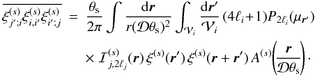 (A.30)To
integrate over angles, we again introduce a Dirac factor
∫dr′′δD(r′′−r−r′)
that we write under its exponential representation, which we expand over spherical
harmonics. Using the expansions (11) and
(A.18), we obtain
(A.30)To
integrate over angles, we again introduce a Dirac factor
∫dr′′δD(r′′−r−r′)
that we write under its exponential representation, which we expand over spherical
harmonics. Using the expansions (11) and
(A.18), we obtain 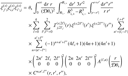 (A.31)where
we introduced the symmetric functions
(A.31)where
we introduced the symmetric functions 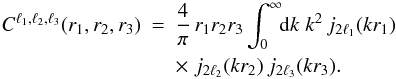 (A.32)For
numerical computations it is more efficient to write Eq. (A.31) in a partially factorized form by exchanging the order of the
integrations and moving the integration over k included in the function
Cℓ1,ℓ2,ℓ3
to the left. Using the decomposition (11)−(14) and integrating over
r′′, this gives
(A.32)For
numerical computations it is more efficient to write Eq. (A.31) in a partially factorized form by exchanging the order of the
integrations and moving the integration over k included in the function
Cℓ1,ℓ2,ℓ3
to the left. Using the decomposition (11)−(14) and integrating over
r′′, this gives 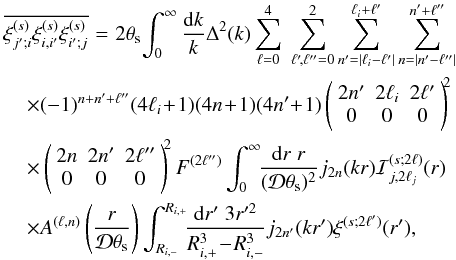 (A.33)where
F(2ℓ′′) is the prefactor in
Eqs. (12)−(14),
(A.33)where
F(2ℓ′′) is the prefactor in
Eqs. (12)−(14),
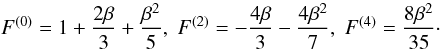 (A.34)Again, all these
geometrical averages of redshift-space correlations reduce to the real-space results of
Valageas et al. (2011), if we set
β = 0 and only keep the monopole terms.
(A.34)Again, all these
geometrical averages of redshift-space correlations reduce to the real-space results of
Valageas et al. (2011), if we set
β = 0 and only keep the monopole terms.
Appendix B: Some useful integrals
We describe here the computation of some of the functions introduced in Appendix A.
B.1. Multipoles of A(s)(y)
Using the expression (A.23) and the
expansion (Gradshteyn & Ryzhik 1994)
 (B.1)we
can write
(B.1)we
can write 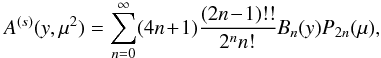 (B.2)with
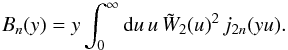 (B.3)This yields the
multipoles
(B.3)This yields the
multipoles 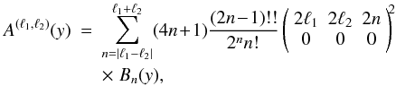 (B.4)and
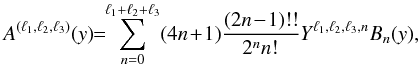 (B.5)with
 (B.6)Because we only
considered the low-order multipoles
0 ≤ ℓi ≤ 2 of the redshift-space
correlation function, we only need the first few multipoles
A(ℓ1,ℓ2)
and
A(ℓ1,ℓ2,ℓ3).
The associated numbers
Yℓ1,ℓ2,ℓ3,ℓ4
and functions Bn(y) can be
computed in advance.
(B.6)Because we only
considered the low-order multipoles
0 ≤ ℓi ≤ 2 of the redshift-space
correlation function, we only need the first few multipoles
A(ℓ1,ℓ2)
and
A(ℓ1,ℓ2,ℓ3).
The associated numbers
Yℓ1,ℓ2,ℓ3,ℓ4
and functions Bn(y) can be
computed in advance.
B.2. Symmetric functions Cℓ1,ℓ2,ℓ3
The functions
Cℓ1,ℓ2,ℓ3
defined in Eq. (A.32) vanish if the
three lengths
{ r1,r2,r3 }
do not obey triangular inequalities. It is also useful to note that these functions obey
the scale invariance  (B.7)For
|r1 − r2| < r3 < r1 + r2,
as in Eq. (A.31), we obtain explicit
expressions using the recursion relations of Bessel functions and the property (Gradshteyn & Ryzhik 1994)
(B.7)For
|r1 − r2| < r3 < r1 + r2,
as in Eq. (A.31), we obtain explicit
expressions using the recursion relations of Bessel functions and the property (Gradshteyn & Ryzhik 1994)  (B.8)for
 (B.9)Indeed,
Eq. (A.32) also reads as
(B.9)Indeed,
Eq. (A.32) also reads as  (B.10)Then,
using the recursion
(B.10)Then,
using the recursion  (B.11)we can lower the
indices
{ ℓ1,ℓ2,ℓ3 }
and can express all required quantities in terms of integrals of the form (B.8) with two identical indices and the
right power-law prefactor. For instance, the first few functions read as
(B.11)we can lower the
indices
{ ℓ1,ℓ2,ℓ3 }
and can express all required quantities in terms of integrals of the form (B.8) with two identical indices and the
right power-law prefactor. For instance, the first few functions read as  were
we defined
were
we defined  (B.15)
 |
Fig. C.1 Contour plots for the redshift-space auto-correlation matrices
|
 |
Fig. C.2 Contour plots for the redshift-space cross-correlation matrices
|
B.3. Functions  (a, b)
To compute the geometrical means of the redshift-space
correlation with respect to bin i, defined in Eq. (A.17), we need the functions
defined in Eq. (A.20). Using Eq. (A.4), they also write as 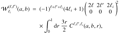 (B.16)where
the functions
Cℓ1,ℓ2,ℓ3
were defined in Eq. (A.32). From the
triangular constraint on these functions
Cℓ1,ℓ2,ℓ3
we obtain
(B.16)where
the functions
Cℓ1,ℓ2,ℓ3
were defined in Eq. (A.32). From the
triangular constraint on these functions
Cℓ1,ℓ2,ℓ3
we obtain  (B.17)while the scale
invariance (B.7) leads to
(B.17)while the scale
invariance (B.7) leads to
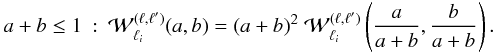 (B.18)Then,
from the explicit expressions obtained in Appendix B.2, which are rational functions of
{ r1,r2,r3 } ,
we can perform the integral (B.16) and
derive explicit expressions. In particular, the first function reads as
(B.18)Then,
from the explicit expressions obtained in Appendix B.2, which are rational functions of
{ r1,r2,r3 } ,
we can perform the integral (B.16) and
derive explicit expressions. In particular, the first function reads as ![Mathematical equation: \appendix \setcounter{section}{2} \begin{eqnarray} \label{W3-s-ell-5} &&|a\!-\!b|<1, \; a\!+\!b<1 : \;\;\; \cW_0^{(0,0)}= 3 a b ,\\ &&|a-b|<1, \; a+b>1 : \;\;\; \cW_0^{(0,0)}= \frac{3}{4} [1-(a-b)^2] . \end{eqnarray}](/articles/aa/full_html/2012/11/aa19646-12/aa19646-12-eq384.png)
Appendix C: Correlation matrices of the “2ℓ = 2” redshift-space correlation
C.1. Auto-correlation of the “2ℓ = 2” multipole
We show in Fig. C.1 the auto-correlation matrices of the “2ℓ = 2” redshift-space correlation. For simplicity we only plot our results for the full matrices that include the non-Gaussian contributions associated with the 3-pt and 4-pt correlation functions. We can see that they are significantly more diagonal than the auto-correlation matrices of the monopole term that were displayed in the right panels of Fig. 8.
C.2. Cross-correlation of the “2ℓ = 2” and “2ℓ = 2” multipoles
We show in Fig. C.2 the cross-correlation
matrices of the “2ℓi = 0” and
“2ℓj = 2” redshift-space correlations.
Thus, in the plane
{ Ri,Rj }
we plot the contour plots of the matrix  (C.1)Because
ℓi ≠ ℓj
this matrix is no longer symmetric in the plane
{ Ri,Rj }
and it can be negative for
Ri = Rj.
We can see that its amplitude is rather small, typically on the order of 0.05, even
along the diagonal. Indeed, because
ℓi ≠ ℓj
the pure shot-noise contribution to Eq. (34) vanishes (the factor
δℓi,ℓj(4ℓi + 1)
within the brackets). This is due to the orthogonality of the Legendre polynomials,
which are the basis of the multipole decomposition of the redshift-space correlation.
The small amplitude of
{ Ri,Rj }
found in Fig. C.2 means that the full covariance
matrix is
approximately block-diagonal in the space
{ Ri,2ℓi } .
Therefore, we may neglect for
ℓi ≠ ℓj
and decouple the analysis of
and .
(C.1)Because
ℓi ≠ ℓj
this matrix is no longer symmetric in the plane
{ Ri,Rj }
and it can be negative for
Ri = Rj.
We can see that its amplitude is rather small, typically on the order of 0.05, even
along the diagonal. Indeed, because
ℓi ≠ ℓj
the pure shot-noise contribution to Eq. (34) vanishes (the factor
δℓi,ℓj(4ℓi + 1)
within the brackets). This is due to the orthogonality of the Legendre polynomials,
which are the basis of the multipole decomposition of the redshift-space correlation.
The small amplitude of
{ Ri,Rj }
found in Fig. C.2 means that the full covariance
matrix is
approximately block-diagonal in the space
{ Ri,2ℓi } .
Therefore, we may neglect for
ℓi ≠ ℓj
and decouple the analysis of
and .
All Figures
|
Fig. 1 Mean redshift-space (solid lines) and real-space (dashed lines) halo correlations,
|
| In the text | |
|
Fig. 2 “2ℓ = 2” redshift-space halo correlation
|
| In the text | |
|
Fig. 3 Redshift-space (solid line, for 2ℓ = 0) and real-space (dashed
line) covariance matrices, |
| In the text | |
|
Fig. 4 Redshift-space (solid line, for 2ℓ = 0) and real-space (dashed
line) covariance matrices, |
| In the text | |
|
Fig. 5 Signal-to-noise ratio of the redshift-space (solid line) and real-space (dashed line) two-point correlations. We show the results obtained for halos in the redshift range 0 < z < 0.8 with an angular window of 50 deg2. |
| In the text | |
|
Fig. 6 Relative importance of the non-Gaussian contributions
|
| In the text | |
|
Fig. 7 Relative importance of the non-Gaussian contributions
|
| In the text | |
|
Fig. 8 Contour plots for the redshift-space correlation matrices
|
| In the text | |
|
Fig. 9 Covariance matrix |
| In the text | |
|
Fig. 10 Covariance matrix |
| In the text | |
|
Fig. 11 Relative importance of the non-Gaussian contributions
|
| In the text | |
|
Fig. 12 Relative importance of the non-Gaussian contributions
|
| In the text | |
|
Fig. 13 Mean monopole redshift-space (solid lines) and real-space (dashed lines)
correlations, |
| In the text | |
|
Fig. 14 Mean monopole correlations, |
| In the text | |
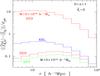 |
Fig. 15 Ratio |
| In the text | |
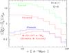 |
Fig. 16 Ratio |
| In the text | |
|
Fig. 17 Mean “2ℓ = 2” redshift-space correlation
|
| In the text | |
|
Fig. 18 Mean “2ℓ = 2” redshift-space correlation
|
| In the text | |
|
Fig. 19 Mean “2ℓ = 4”redshift-space correlation
|
| In the text | |
|
Fig. C.1 Contour plots for the redshift-space auto-correlation matrices
|
| In the text | |
|
Fig. C.2 Contour plots for the redshift-space cross-correlation matrices
|
| In the text | |
Current usage metrics show cumulative count of Article Views (full-text article views including HTML views, PDF and ePub downloads, according to the available data) and Abstracts Views on Vision4Press platform.
Data correspond to usage on the plateform after 2015. The current usage metrics is available 48-96 hours after online publication and is updated daily on week days.
Initial download of the metrics may take a while.