© ESO, 2012

1. Introduction

Gravitational lensing effects provide versatile tools for probing the matter distribution in the Universe. Galaxy-galaxy lensing (GGL), for example, is a statistical approach using lensing to obtain information on the mass associated with individual galaxies (see, e.g., Bartelmann & Schneider 2001). This is achieved by dividing the galaxy population into lenses (foreground) and sources (background). The images of the sources are sheared due to the gravitational field of the foreground lenses and their surrounding mass. The image shearing is usually too small to be detected for individual source-lens galaxy pairs. Instead, the lensing effect is measured as a correlation between the observed image ellipticities and the lens positions. The signal obtained from averaging over many source-lens pairs can then be related to the average mass profiles of the lenses.

Since its first detection (Brainerd et al. 1996), GGL has been measured in many large galaxy surveys (e.g., Hoekstra et al. 2002; Kleinheinrich et al. 2006; Mandelbaum et al. 2006; Simon et al. 2008; van Uitert et al. 2011, and references therein). Schneider & Watts (2005) advanced GGL to galaxy-galaxy-galaxy lensing (G3L) by introducing third-order correlation functions that involve either configurations with two background sources and one lens galaxy (G _± ), or with two lenses and one background source . The latter measures the lensing signal around pairs of lens galaxies in excess of what one obtains by simply adding the average signals of two individual galaxies, and thus provides a measure of the excess matter profile about clustered lens galaxy pairs (Simon et al. 2012). This G3L signal has been measured in the Red sequence Cluster Survey (RCS, Gladders & Yee 2005) by Simon et al. (2008), who indeed found an excess mass about lens pairs with projected separation of 250   h^-1   kpc. The GG(G)L correlations can be converted to aperture statistics (which we utilize in this work), providing a convenient probe of the galaxy-matter power(bi-)spectra at particular scales.

The galaxy-mass correlation as seen by weak lensing can also be studied theoretically by combining dark matter simulations with semi-analytic models (SAM) of galaxy evolution (White & Frenk 1991; Kauffmann et al. 1999; Springel et al. 2001). In this approach, the dark matter halos of an N-body simulation of cosmic structure formation are populated with galaxies. The properties of the galaxies are calculated by combining information on the halo merger trees of the underlying dark matter simulation with an analytic model of the gas physics in galaxies. The physical processes considered include gas cooling, star formation, metal enrichment, and feedback due to supernovae and active galactic nuclei. Using ray-tracing (e.g. Hilbert et al. 2009), one can then simulate lensing observations of the resulting galaxy distribution.

This paper provides a study of the second- and third-order galaxy-mass correlations in semi-analytic galaxy formation models as probed by lensing via aperture statistics (Schneider 1996; Schneider et al. 1998). We consider two models based on the Millennium Run (Springel et al. 2005): the Durham model by Bower et al. (2006) and the Garching model by Guo et al. (2011). We find that the predicted second- and third-order lensing signals differ between galaxies of different color and magnitude, but also between the different galaxy models. The differences between the models can be traced back to, among other things, different treatments of the satellite galaxy evolution. This illustrates that galaxy-galaxy(-galaxy) lensing can be a sensitive probe of galaxy evolution.

The outline of the paper is as follows: Sect. 2 provides a brief account of gravitational lensing, aperture statistics, and their relation to correlation functions. Our lensing simulations and the method we use to measure aperture statistics (a fast method based on Fast Fourier Transforms) are described in Sect. 3. The results of these measurements for different subsets of galaxies, defined by redshift, luminosity or color, are presented in Sect. 4. The main part of the paper concludes with a summary and discussion in Sect. 5. In the appendix, we briefly discuss shot-noise corrections for the aperture statistics.

2. Theory

2.1. Gravitational lensing basics

The matter density inhomogeneities can be quantified by the dimensionless density contrast ${\mathit{\delta }}_{\mathrm{m}}\left({x}\mathit{,\chi }\right)\mathrm{=}\frac{{\mathit{\rho }}_{\mathrm{m}}\left({x}\mathit{,\chi }\right)\mathrm{-}\mathit{\rho ̅}\mathrm{m}\mathrm{\left(}\mathit{\chi }\mathrm{\right)}}{\mathit{\rho ̅}\mathrm{m}\mathrm{\left(}\mathit{\chi }\mathrm{\right)}}\mathit{,}$(1)where ρ_m(x,χ) is the spatial matter density at comoving transverse position x and comoving radial distance χ, and  denotes the mean density at that distance. To lowest order, the convergence κ_m for sources at comoving distance χ is related to the matter density contrast δ_m by the projection along the line-of-sight by (e.g. Schneider et al. 2006) ${\mathit{\kappa }}_{\mathrm{m}}\left({\vartheta }\mathit{,\chi }\right)\mathrm{=}\frac{\mathrm{3}{\mathit{H}}_{\mathrm{0}}^{\mathrm{2}}{\mathrm{\Omega }}_{\mathrm{m}}}{\mathrm{2}{\mathit{c}}^{\mathrm{2}}}{\mathrm{\int }}_{\mathrm{0}}^{\mathit{\chi }}\mathrm{d}{\mathit{\chi }}^{\mathrm{\prime }}\hspace{0.17em}\frac{{\mathit{f}}_{\mathit{K}}\left(\mathit{\chi }\mathrm{-}{\mathit{\chi }}^{\mathrm{\prime }}\right){\mathit{f}}_{\mathit{K}}\left({\mathit{\chi }}^{\mathrm{\prime }}\right)}{{\mathit{f}}_{\mathit{K}}\mathrm{\left(}\mathit{\chi }\mathrm{\right)}}\frac{{\mathit{\delta }}_{\mathrm{m}}\left({\mathit{f}}_{\mathit{K}}\left({\mathit{\chi }}^{\mathrm{\prime }}\right){\vartheta }\mathit{,}{\mathit{\chi }}^{\mathrm{\prime }}\right)}{\mathit{a}\left({\mathit{\chi }}^{\mathrm{\prime }}\right)}\mathit{,}$(2)where κ_m describes the dimensionless projected matter density, H₀ denotes the Hubble constant, Ω_m the mean matter density parameter, c the speed of light, f_K(χ) the comoving angular diameter distance, and a(χ) = 1/(1 + z(χ)) the scale factor at redshift z(χ).

For a distribution of sources with probability density p_s(χ), the effective convergence is given by $\begin{array}{ccc}{\mathit{\kappa }}_{\mathrm{m}}\left({\vartheta }\right)& \mathrm{=}& \int \mathrm{d}\mathit{\chi }\hspace{0.17em}{\mathit{p}}_{\mathrm{s}}\left(\mathit{\chi }\right)\hspace{0.17em}{\mathit{\kappa }}_{\mathrm{m}}\left({\vartheta }\mathit{,\chi }\right)\\ & \mathrm{=}& \int \mathrm{d}\mathit{\chi }\hspace{0.17em}\mathit{g}\left(\mathit{\chi }\right){\mathit{\delta }}_{\mathrm{m}}\left({\mathit{f}}_{\mathit{K}}\left(\mathit{\chi }\right){\vartheta }\mathit{,\chi }\right) \mathrm{with}\\ \mathit{g}\left(\mathit{\chi }\right)& \mathrm{=}& \frac{\mathrm{3}{\mathit{H}}_{\mathrm{0}}^{\mathrm{2}}{\mathrm{\Omega }}_{\mathrm{m}}}{\mathrm{2}{\mathit{c}}^{\mathrm{2}}}\frac{{\mathit{f}}_{\mathit{K}}\left(\mathit{\chi }\right)}{\mathit{a}\left(\mathit{\chi }\right)}{\mathrm{\int }}_{\mathit{\chi }}^{\mathrm{\infty }}\mathrm{d}{\mathit{\chi }}^{\mathrm{\prime }}\hspace{0.17em}{\mathit{p}}_{\mathit{\chi }}\left({\mathit{\chi }}^{\mathrm{\prime }}\right)\frac{{\mathit{f}}_{\mathit{K}}\left({\mathit{\chi }}^{\mathrm{\prime }}\mathrm{-}\mathit{\chi }\right)}{{\mathit{f}}_{\mathit{K}}\left({\mathit{\chi }}^{\mathrm{\prime }}\right)}\mathrm{·}\end{array}$Similar to the definition of the dimensionless matter density contrast δ_m, one can define the number density contrast δ_g of the lens galaxies as ${\mathit{\delta }}_{\mathrm{g}}\left({x}\mathit{,\chi }\right)\mathrm{=}\frac{{\mathit{\rho }}_{\mathrm{g}}\left({x}\mathit{,\chi }\right)\mathrm{-}\mathit{\rho ̅}\mathrm{g}\left(\mathit{\chi }\right)}{\mathit{\rho ̅}\mathrm{g}\left(\mathit{\chi }\right)}\mathit{,}$(5)where ρ_g(x,χ) is the number density of the lens galaxies at comoving transverse position x and distance χ, and  is mean number density of lens galaxies at comoving distance χ. Using the projected number density ${\mathit{n}}_{\mathrm{g}}\left({\vartheta }\right)\mathrm{=}\mathrm{\int }\mathrm{d}\mathit{\chi }{\mathit{f}}_{\mathit{K}}^{\mathrm{2}}\left(\mathit{\chi }\right)\hspace{0.17em}{\mathit{\rho }}_{\mathrm{g}}\left({\mathit{f}}_{\mathit{K}}\left(\mathit{\chi }\right){\vartheta }\mathit{,\chi }\right)$(6)and the mean projected number density $\mathit{n̅}\mathrm{g}\mathrm{=}\mathrm{\int }\mathrm{d}\mathit{\chi }{\mathit{f}}_{\mathit{K}}^{\mathrm{2}}\left(\mathit{\chi }\right)\hspace{0.17em}\mathit{\rho ̅}\mathrm{g}\left(\mathit{\chi }\right)\mathit{,}$(7)the projected number density contrast for lens galaxies with distance distribution ${\mathit{p}}_{\mathrm{g}}\mathrm{\left(}\mathit{\chi }\mathrm{\right)}\mathrm{=}\mathit{n̅}\begin{array}{}-1\\ \mathrm{g}\end{array}{\mathit{f}}_{\mathit{K}}^{\mathrm{2}}\mathrm{\left(}\mathit{\chi }\mathrm{\right)}\hspace{0.17em}\mathit{\rho ̅}{}_{\mathrm{g}}\mathrm{\left(}\mathit{\chi }\mathrm{\right)}$ can be computed by $\begin{array}{ccc}{\mathit{\kappa }}_{\mathrm{g}}\left({\vartheta }\right)\mathrm{=}\frac{{\mathit{n}}_{\mathrm{g}}\left({\vartheta }\right)\mathrm{-}\mathit{n̅}\mathrm{g}}{\mathit{n̅}\mathrm{g}}\mathrm{=}\mathrm{\int }\mathrm{d}\mathit{\chi }\hspace{0.17em}{\mathit{p}}_{\mathrm{g}}\left(\mathit{\chi }\right){\mathit{\delta }}_{\mathrm{g}}\left({\mathit{f}}_{\mathit{K}}\left(\mathit{\chi }\right){\vartheta }\mathit{,\chi }\right)\mathit{.}& & \end{array}$(8)

2.2. Aperture statistics

Aperture statistics was originally introduced as a way to quantify the surface mass density that is unaffected by the mass sheet degeneracy (Schneider 1996). The aperture mass is defined as a convolution, ${\mathit{M}}_{\mathrm{ap}}\left({\vartheta }\mathrm{;}\mathit{\theta }\right)\mathrm{=}\mathrm{\int }{\mathrm{d}}^{\mathrm{2}}{{\vartheta }}^{\mathrm{\prime }}\hspace{0.17em}{\mathit{U}}_{\mathit{\theta }}\mathrm{(}{\left|{\vartheta }\mathrm{-}{{\vartheta }}^{\mathrm{\prime }}\right|}^{\mathrm{)}}\hspace{0.17em}{\mathit{\kappa }}_{\mathrm{m}}\left({{\vartheta }}^{\mathrm{\prime }}\right)\mathit{,}$(9)of the convergence κ and an axi-symmetric filter U_θ( | ϑ | ) whose size is given by the scale θ, and that is compensated, i.e. $\mathrm{\int }\mathrm{d}\mathit{\vartheta }\hspace{0.17em}\mathit{\vartheta }\hspace{0.17em}{\mathit{U}}_{\mathit{\theta }}\mathrm{(}{\mathit{\vartheta }}^{\mathrm{)}}\mathrm{=}\mathrm{0.}$(10)In this work, we use the filter introduced by Crittenden et al. (2002), $\begin{array}{ccc}{\mathit{U}}_{\mathit{\theta }}\mathrm{(}{\mathit{\vartheta }}^{\mathrm{)}}& \mathrm{=}& \frac{\mathrm{1}}{\mathrm{2}\mathit{\pi }{\mathit{\theta }}^{\mathrm{2}}}\left[\mathrm{1}\mathrm{-}\frac{{\mathit{\vartheta }}^{\mathrm{2}}}{\mathrm{2}{\mathit{\theta }}^{\mathrm{2}}}\right]\exp \left(\frac{\mathrm{-}{\mathit{\vartheta }}^{\mathrm{2}}}{\mathrm{2}{\mathit{\theta }}^{\mathrm{2}}}\right)\mathrm{=}\frac{\mathrm{1}}{{\mathit{\theta }}^{\mathrm{2}}}\hspace{0.17em}\mathit{u}\left(\frac{\mathit{\vartheta }}{\mathit{\theta }}\right) \mathrm{with}\\ \mathit{u}\mathrm{\left(}\mathit{x}\mathrm{\right)}& \mathrm{=}& \frac{\mathrm{1}}{\mathrm{2}\mathit{\pi }}\left[\mathrm{1}\mathrm{-}\frac{{\mathit{x}}^{\mathrm{2}}}{\mathrm{2}}\right]\exp \left(\frac{\mathrm{-}{\mathit{x}}^{\mathrm{2}}}{\mathrm{2}}\right)\mathrm{·}\end{array}$Its (2D) Fourier transform has a simple analytical form $\begin{array}{ccc}\begin{array}{}\mathrm{˜}\\ {\mathit{U}}_{\mathit{\theta }}\end{array}\mathrm{(}{\mathit{\ell }}^{\mathrm{)}}& \mathrm{=}& \int {\mathrm{d}}^{\mathrm{2}}{\vartheta }\hspace{0.17em}{\mathit{U}}_{\mathit{\theta }}\left(\left|{\vartheta }\right|\right)\hspace{0.17em}{\mathrm{e}}^{\mathrm{i}{\ell }\mathrm{·}{\vartheta }}\mathrm{=}\frac{{\mathit{\theta }}^{\mathrm{2}}{\mathit{\ell }}^{\mathrm{2}}}{\mathrm{2}}\hspace{0.17em}{\mathrm{e}}^{\mathrm{-}\frac{\mathrm{1}}{\mathrm{2}}{\mathit{\theta }}^{\mathrm{2}}{\mathit{\ell }}^{\mathrm{2}}}\mathrm{=}\begin{array}{}\mathrm{˜}\\ \mathit{u}\end{array}\mathrm{(}\mathit{\theta }{\mathit{\ell }}^{\mathrm{)}} \mathrm{with}\\ \begin{array}{}\mathrm{˜}\\ \mathit{u}\end{array}\mathrm{\left(}\mathit{k}\mathrm{\right)}& \mathrm{=}& \frac{{\mathit{k}}^{\mathrm{2}}}{\mathrm{2}}\exp \left(\frac{\mathrm{-}{\mathit{k}}^{\mathrm{2}}}{\mathrm{2}}\right)\mathrm{·}\end{array}$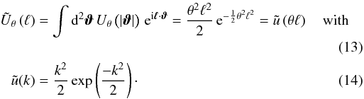The filter falls off exponentially for ϑ ≫ θ. This makes the support of the filter finite in practice.

In analogy to the aperture mass M_ap, one can define the aperture number count $\mathrm{𝒩}\left({\vartheta }\mathrm{;}\mathit{\theta }\right)\mathrm{=}\mathrm{\int }{\mathrm{d}}^{\mathrm{2}}{{\vartheta }}^{\mathrm{\prime }}\hspace{0.17em}{\mathit{U}}_{\mathit{\theta }}\mathrm{(}{\left|{\vartheta }\mathrm{-}{{\vartheta }}^{\mathrm{\prime }}\right|}^{\mathrm{)}}\hspace{0.17em}{\mathit{\kappa }}_{\mathrm{g}}\left({{\vartheta }}^{\mathrm{\prime }}\right)\mathit{.}$(15)The aperture number count dispersion is related to the angular two-point correlation function ${\mathit{w}}_{\mathrm{gg}}\left(\left|{{\vartheta }}_{\mathrm{2}}\mathrm{-}{{\vartheta }}_{\mathrm{1}}\right|\right)\mathrm{=}\mathrm{⟨}{{\mathit{\kappa }}_{\mathrm{g}}\left({{\vartheta }}_{\mathrm{1}}\right){\mathit{\kappa }}_{\mathrm{g}}\left({{\vartheta }}_{\mathrm{2}}\right)}^{\mathrm{⟩}}\mathit{,}$(16)and its Fourier transform, the angular power spectrum P_gg(ℓ) of the lens galaxies, through $\begin{array}{ccc}⟨{\mathrm{𝒩}}^{\mathrm{2}}⟩\mathrm{\left(}\mathit{\theta }\mathrm{\right)}& \mathrm{\equiv }& ⟨\mathrm{𝒩}\left({\vartheta }\mathrm{;}\mathit{\theta }\right)\mathrm{𝒩}\left({\vartheta }\mathrm{;}\mathit{\theta }\right)⟩\\ & \mathrm{=}& \int {\mathrm{d}}^{\mathrm{2}}{{\vartheta }}_{\mathrm{1}}\hspace{0.17em}{\mathit{U}}_{\mathit{\theta }}\left(\left|{{\vartheta }}_{\mathrm{1}}\right|\right)\hspace{0.17em}\mathrm{\int }{\mathrm{d}}^{\mathrm{2}}{{\vartheta }}_{\mathrm{2}}\hspace{0.17em}{\mathit{U}}_{\mathit{\theta }}\left(\left|{{\vartheta }}_{\mathrm{2}}\right|\right)\hspace{0.17em}{\mathit{w}}_{\mathrm{gg}}\left(\mathrm{|}{{\vartheta }}_{\mathrm{2}}\mathrm{-}{{\vartheta }}_{\mathrm{1}}\mathrm{|}\right)\\ & \mathrm{=}& {\mathrm{\int }}_{\mathrm{0}}^{\mathrm{\infty }}\frac{\mathit{\ell }\mathrm{d}\mathit{\ell }}{\mathrm{2}\mathit{\pi }}\stackrel{}{{{\mathit{u}}^{\mathrm{2}}}_{\mathrm{˜}}}\mathrm{\left(}\mathit{\theta \ell }\mathrm{\right)}{\mathit{P}}_{\mathrm{gg}}\mathrm{\left(}\mathit{\ell }\mathrm{\right)}\mathit{.}\end{array}$(17)The function $\begin{array}{}{}_{\mathrm{˜}}\\ \mathit{u}\end{array}\mathrm{\left(}\mathit{\ell \theta }\mathrm{\right)}$ features a sharp peak at $\mathit{\ell \theta }\mathrm{=}\sqrt{\mathrm{2}}$. Thus, provides a measurement of the corresponding power spectrum P_gg(ℓ) at wave numbers ℓ ~ 1/θ.

Within the halo model framework of cosmic structure (e.g. Cooray & Sheth 2002), on small scales θ probes the distribution of the lens galaxies within individual dark matter halos. On large scales, provides a probe of the clustering of the host halos of the lens galaxies.

Correlating M_ap(θ) with yields $\begin{array}{ccc}\mathrm{⟨}{\mathrm{𝒩}{\mathit{M}}_{\mathrm{ap}}}^{\mathrm{⟩}}\mathrm{\left(}\mathit{\theta }\mathrm{\right)}& \mathrm{\equiv }\mathrm{⟨}{\mathrm{𝒩}\left({\vartheta }\mathrm{;}\mathit{\theta }\right){\mathit{M}}_{\mathrm{ap}}\left({\vartheta }\mathrm{;}\mathit{\theta }\right)}^{\mathrm{⟩}}& \\ & \mathrm{=}& \int {\mathrm{d}}^{\mathrm{2}}{{\vartheta }}_{\mathrm{1}}\hspace{0.17em}{\mathit{U}}_{\mathit{\theta }}\left(\left|{{\vartheta }}_{\mathrm{1}}\right|\right)\hspace{0.17em}\mathrm{\int }{\mathrm{d}}^{\mathrm{2}}{{\vartheta }}_{\mathrm{2}}\hspace{0.17em}{\mathit{U}}_{\mathit{\theta }}\left(\left|{{\vartheta }}_{\mathrm{2}}\right|\right){\mathit{w}}_{\mathrm{gm}}\left(\mathrm{|}{{\vartheta }}_{\mathrm{2}}\mathrm{-}{{\vartheta }}_{\mathrm{1}}\mathrm{|}\right)\\ & \mathrm{=}& {\mathrm{\int }}_{\mathrm{0}}^{\mathrm{\infty }}\frac{\mathit{\ell }\mathrm{d}\mathit{\ell }}{\mathrm{2}\mathit{\pi }}\stackrel{}{{{\mathit{u}}^{\mathrm{2}}}_{\mathrm{˜}}}\mathrm{\left(}\mathit{\theta \ell }\mathrm{\right)}{\mathit{P}}_{\mathrm{gm}}\mathrm{\left(}\mathit{\ell }\mathrm{\right)}\mathit{,}\end{array}$(18)with w_gm( | ϑ₂ − ϑ₁ | ) = ⟨κ_g(ϑ₁)κ_m(ϑ₂)⟩, whose Fourier transform is the cross-power spectrum of galaxies and convergence P_gm. The galaxy-galaxy lensing aperture statistics probes the average matter profiles around lens galaxies.

A third-order aperture correlator (Schneider & Watts 2005) is obtained by $\begin{array}{ccc}\mathrm{⟨}{{\mathrm{𝒩}}^{\mathrm{2}}{\mathit{M}}_{\mathrm{ap}}}^{\mathrm{⟩}}\mathrm{\left(}\mathit{\theta }\mathrm{\right)}& \mathrm{\equiv }& \mathrm{⟨}{\mathrm{𝒩}\left({\vartheta }\mathrm{;}\mathit{\theta }\right)\mathrm{𝒩}\left({\vartheta }\mathrm{;}\mathit{\theta }\right){\mathit{M}}_{\mathrm{ap}}\left({\vartheta }\mathrm{;}\mathit{\theta }\right)}^{\mathrm{⟩}}\\ & \mathrm{=}& \int {\mathrm{d}}^{\mathrm{2}}{{\vartheta }}_{\mathrm{1}}\hspace{0.17em}{\mathit{U}}_{\mathit{\theta }}\left(\left|{{\vartheta }}_{\mathrm{1}}\right|\right)\hspace{0.17em}\mathrm{\int }{\mathrm{d}}^{\mathrm{2}}{{\vartheta }}_{\mathrm{2}}\hspace{0.17em}{\mathit{U}}_{\mathit{\theta }}\left(\left|{{\vartheta }}_{\mathrm{2}}\right|\right)\\ & & \mathrm{\times }\mathrm{\int }{\mathrm{d}}^{\mathrm{2}}{{\vartheta }}_{\mathrm{3}}\hspace{0.17em}{\mathit{U}}_{\mathit{\theta }}\left(\left|{{\vartheta }}_{\mathrm{3}}\right|\right)\mathrm{⟨}{\mathit{\kappa }}_{\mathrm{g}}\left({{\vartheta }}_{\mathrm{1}}\right){\mathit{\kappa }}_{\mathrm{g}}\left({{\vartheta }}_{\mathrm{2}}\right)\mathit{\kappa }{\left({{\vartheta }}_{\mathrm{3}}\right)}^{\mathrm{⟩}}\\ & \mathrm{=}& \int \frac{{\mathrm{d}}^{\mathrm{2}}{{\ell }}_{\mathrm{1}}}{\mathrm{(}\mathrm{2}\mathit{\pi }{\mathrm{)}}^{\mathrm{2}}}\mathrm{\int }\frac{{\mathrm{d}}^{\mathrm{2}}{{\ell }}_{\mathrm{2}}}{\mathrm{(}\mathrm{2}\mathit{\pi }{\mathrm{)}}^{\mathrm{2}}}\hspace{0.17em}\begin{array}{}\mathrm{˜}\\ \mathit{u}\end{array}\left(\mathit{\theta }\left|{{\ell }}_{\mathrm{1}}\right|\right)\hspace{0.17em}\begin{array}{}\mathrm{˜}\\ \mathit{u}\end{array}\left(\mathit{\theta }\left|{{\ell }}_{\mathrm{2}}\right|\right)\hspace{0.17em}\begin{array}{}\mathrm{˜}\\ \mathit{u}\end{array}\left(\mathit{\theta }\left|{{\ell }}_{\mathrm{1}}\mathrm{+}{{\ell }}_{\mathrm{2}}\right|\right)\\ & & \mathrm{\times }{\mathit{B}}_{\mathrm{ggm}}\mathrm{(}{{\ell }}_{\mathrm{1}}\mathit{,}{{\ell }}_{\mathrm{2}}\mathit{,}\mathrm{-}{{\ell }}_{\mathrm{1}}\mathrm{-}{{\ell }}_{\mathrm{2}}\mathrm{)}\end{array}$(19)where the last line contains the angular bispectrum of the projected quantities (Schneider & Watts 2005), $⟨\begin{array}{}\mathrm{˜}\\ {\mathit{\kappa }}_{\mathrm{1}}\end{array}\mathrm{\left(}{{\ell }}_{\mathrm{1}}\mathrm{\right)}\begin{array}{}\mathrm{˜}\\ {\mathit{\kappa }}_{\mathrm{2}}\end{array}\mathrm{\left(}{{\ell }}_{\mathrm{2}}\mathrm{\right)}\begin{array}{}\mathrm{˜}\\ {\mathit{\kappa }}_{\mathrm{3}}\end{array}\mathrm{\left(}{{\ell }}_{\mathrm{3}}\mathrm{\right)}⟩\mathrm{=}\mathrm{(}\mathrm{2}\mathit{\pi }{\mathrm{)}}^{\mathrm{2}}{\mathit{\delta }}_{\mathrm{D}}\mathrm{(}{{\ell }}_{\mathrm{1}}\mathrm{+}{{\ell }}_{\mathrm{2}}\mathrm{+}{{\ell }}_{\mathrm{3}}\mathrm{)}{\mathit{B}}_{\mathrm{123}}\mathrm{\left(}{{\ell }}_{\mathrm{1}}\mathit{,}{{\ell }}_{\mathrm{2}}\mathit{,}{{\ell }}_{\mathrm{3}}\mathrm{\right)}\mathit{.}$(20)On small scales, can teach us about the average mass distribution of halos hosting two lens galaxies. On larger scales, also provides information on the higher-order clustering of the host halos.

2.3. Relative galaxy bias

Clusters and galaxies are biased tracers of the matter distribution (Kaiser 1984; Bardeen et al. 1986; Mo et al. 1996). In the simplest conceivable non-trivial bias model, the bias can be expressed as a linear deterministic relation between the galaxy density contrast and the matter density contrast, ${\mathit{\delta }}_{\mathrm{g}}\left({x}\mathit{,\chi }\right)\mathrm{=}{\mathit{b}}_{\mathrm{gm}}{\mathit{\delta }}_{\mathrm{m}}\left({x}\mathit{,\chi }\right)\mathit{,}$(21)with a bias factor b_gm that does not depend on time or scale, but only on the galaxy sample in question.

A more realistic assumption is that the galaxy bias is stochastic and depends on the time and spatial scale. At the two-point level, the bias may then be quantified by a scale-dependent bias factor and correlation factor. A description of the relation between the galaxy and matter densities at the three-point level or higher requires additional, higher-order bias and correlation parameters.

Aperture statistics can be used to constrain the galaxy bias (Schneider 1998; van Waerbeke 1998; Hoekstra et al. 2002; Schneider & Watts 2005; Simon et al. 2007; Jullo et al. 2012). For example, assuming a linear deterministic bias, , , and . For two lens galaxy samples with identical redshift distributions, but different bias parameters b₁ and b₂, one can then determine the relative bias b₁/b₂ from the aperture statistics $⟨{\mathrm{𝒩}}_{\mathrm{1}\mathit{/}\mathrm{2}}^{\mathrm{2}}⟩$, , and $⟨{\mathrm{𝒩}}_{\mathrm{1}\mathit{/}\mathrm{2}}^{\mathrm{2}}{\mathit{M}}_{\mathrm{ap}}⟩$ of the two lens samples by using any of $\begin{array}{ccc}\frac{{\mathit{b}}_{\mathrm{1}}}{{\mathit{b}}_{\mathrm{2}}}\mathrm{=}\sqrt{\frac{⟨{\mathrm{𝒩}}_{\mathrm{1}}^{\mathrm{2}}⟩\mathrm{\left(}\mathit{\theta }\mathrm{\right)}}{⟨{\mathrm{𝒩}}_{\mathrm{2}}^{\mathrm{2}}⟩\mathrm{\left(}\mathit{\theta }\mathrm{\right)}}}\mathrm{=}\frac{⟨{\mathrm{𝒩}}_{\mathrm{1}}{\mathit{M}}_{\mathrm{ap}}⟩\mathrm{\left(}\mathit{\theta }\mathrm{\right)}}{⟨{\mathrm{𝒩}}_{\mathrm{2}}{\mathit{M}}_{\mathrm{ap}}⟩\mathrm{\left(}\mathit{\theta }\mathrm{\right)}}\mathrm{=}\sqrt{\frac{⟨{\mathrm{𝒩}}_{\mathrm{1}}^{\mathrm{2}}{\mathit{M}}_{\mathrm{ap}}⟩\mathrm{\left(}\mathit{\theta }\mathrm{\right)}}{⟨{\mathrm{𝒩}}_{\mathrm{2}}^{\mathrm{2}}{\mathit{M}}_{\mathrm{ap}}⟩\mathrm{\left(}\mathit{\theta }\mathrm{\right)}}}\mathrm{·}& & \end{array}$(22)If the measured ratios of the aperture statistics change with scale θ, one can extend the idea to a measurement of a scale-dependent bias. For lens galaxy samples with narrow redshift distributions and deterministic bias, the above ratios still agree (roughly) when compared on the same scales. If the galaxy bias is stochastic or non-linear (Dekel & Lahav 1999), however, the ratios from the different statistics disagree even if measured on the same scale. In that case, the second- and third-order aperture statistics each contain valuable independent information on the second- and third-order bias of the galaxies (Schneider & Watts 2005).

3. Methods

3.1. Lensing simulations

For our analysis we use the data obtained by ray-tracing through the Millennium Run (Springel et al. 2005). The Millennium Run (MR) is a large N-body simulation of structure formation in a flat ΛCDM universe with matter density Ω_m = 0.25, baryon density Ω_b = 0.045, dark-energy density Ω_Λ = 0.75, a Hubble constant H₀ = h100   km   s^-1   Mpc^-1 with h = 0.73, and with a power spectrum normalization σ₈ = 0.9. It follows the evolution of N_p ~ 10¹⁰ dark matter particles with mass m_p = 8.6 × 10⁸   h^-1   M_⊙ in a cubic region of comoving side length 500   h^-1   Mpc from redshift z = 127 to the present.

The simulation volume of the MR is large enough to include massive rare objects, yet with sufficiently high spatial and mass resolution to resolve dark matter halos of galaxies. This allows the construction of merger trees of dark matter halos and subhalos within them. These merger trees have been used in various semi-analytic galaxy formation models to calculate the properties of galaxies in the simulation. Here we consider the Durham model by Bower et al. (2006) and the Garching model by Guo et al. (2011)¹. Both models have similar treatments of, e.g., gas cooling and star formation, but differ in various details (see the original papers for a full description). The models have been adjusted to be consistent with a large number of observations, in particular the luminosities, stellar masses, morphologies, gas contents and correlations of galaxies at low redshift, but they have not been tuned to match galaxy properties at higher redshift. We make use of the public Millennium Simulations Database² (Lemson & Virgo Consortium 2006) to obtain the properties of the galaxies predicted by the two models.

We employ the multiple-lens-plane ray-tracing algorithm described in Hilbert et al. (2009) to calculate the light propagation through the matter in the MR. We generate 64 simulated 4 × 4   deg² fields of view. For each field, we calculate the convergence to sources at a number of redshifts on a regular mesh of 4096² pixels, as well as the apparent sky positions, redshifts, and magnitudes of the model galaxies from the Garching and Durham models. The galaxy properties are then used to select various subsamples of the full mock galaxy catalogs as lens populations for the GG(G)L.

3.2. Computing aperture statistics

We introduce a fast method to perform aperture statistics measurements on the 64 simulated fields. The statistic used here is built on two main components: (i) the pixelized convergence field κ_m(ϑ) of the source galaxies on square meshes of 4096² pixels, and (ii) the pixelized lens galaxy number density fields on meshes with the same geometry. The convergence fields are obtained directly from the ray-tracing algorithm. The galaxy density fields are obtained by projecting the apparent position of the lens galaxies in the fields and counting the number of galaxies in each pixel. Finally, dividing by the mean number density of lens galaxies across all 64 fields results in the galaxy number density contrast κ_g(ϑ).

We calculate the aperture statistics M_ap(ϑ;θ) and from κ_m and κ_g on a grid by exploiting the convolution theorem, using fast Fourier transforms (FFT, in particular the FFTW library by Frigo & Johnson 2005) to carry out the convolution in Eqs. (9)and (15). To measure M_ap (or ), we calculate the Fourier transforms of κ_m (or κ_g) and U_θ( | ϑ | ). We then multiply the results in the Fourier space. Finally an inverse Fourier transformation gives M_ap (or ). The number of grid points in the field is finite (4096 × 4096 pixels). Therefore, a “Discrete Fourier Transform” is performed by using the Fast Fourier Transform (FFT) algorithm which reduces an O(N²) process to O(N   log ₂N), with N being the number of points being Fourier transformed. Hence, FFT reduces the computation time immensely.

Since M_ap(ϑ;θ) and fields are not periodic, we exclude points closer than 4θ to the field edges from the subsequent analysis. On the remaining points, we then calculate , , and , and estimate , , and  from these products by spatial averaging. We correct the estimates involving  for shot noise as described in Appendix A.

The G3L statistics can also be calculated from the shear field corresponding to κ_m and the positions of the lens galaxies. In particular, Schneider & Watts (2005) and Simon et al. (2008) showed that can be obtained as an integral over a three-point correlation function (3PCF). In order to check our procedure, we use 32 randomly selected simulated fields and calculate  also with the latter method, by first calculating this 3PCF with the help of a tree code. We note that, while this tree method is more flexible than the simple FFT-based method described above, in particular with regard to field boundaries and gaps, it is also considerably slower.

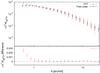Fig. 1 Upper panel: aperture statistics as a function of filter scale θ measured in the Garching model. The FFT method (squares) and the tree method (triangles) are compared for lenses at redshift z = 0.17 with mr ≤ 22.5, stellar masses M⋆ ≥ 109   h-1   M⊙ and convergence field of sources at redshift z = 0.99. Error bars indicate the standard deviation of for aperture radius θ estimated across 32 fields. Lower panel: average difference signal between the FFT method and the tree method. Again the error bars show the standard deviation of the mean (field variance of difference signal divided by $\sqrt{\mathrm{31}}$).

For some of the individual fields, we find fairly large discrepancies between the results from the FFT and the tree method – in particular for fields with a large matter overdensity near the field boundaries. We can attribute these discrepancies to the different ways in which the three-point information is weighted in the two approaches. For example, a triplet of points near the boundary of the field enters the statistics in the tree method with the same weight as a similar triplet near the field center. In contrast, the FFT method, by excluding the stripe at the field boundary, assigns zero weight to such a triple. Hence, the results on individual fields can be quite different.

Both methods are consistent, however, when averaging the results over many fields. Randomly selecting 32 simulated fields, we measure using the FFT method and the tree method. In the upper panel of Fig. 1, the outcomes of the two methods are compared, showing good agreement between the results. The error bars, indicating the statistical error on the signal, tend to be smaller for the tree method than for the FFT method (for apertures larger than 2 arcmin), since the tree method makes better use of the fields’ area. For example, for apertures larger than 20 arcmin, more than half of the field is not included in the FFT measurement. Consequently, the difference in scatter becomes more prominent on larger scales. The lower panel in Fig. 1 shows the field-by-field difference signal averaged over all fields. The difference between the methods is consistent with zero for θ ≥ 1   arcmin, but deviates from zero for θ < 1   arcmin. This is due to a systematic underestimation of the signal in the tree method on small scales (Simon et al. 2008).

4. Results

4.1. Main lens samples

In this section, we present results for the second- and third-order aperture cross-correlations and aperture number count dispersion for the Durham and the Garching model in the 64 simulated fields created from the Millennium Run. For simplicity, the background population is chosen to be located at z = 0.99. Unless stated otherwise, lens galaxies are selected to have redshifts 0.14 ≤ z ≤ 0.62, observer-frame r-band apparent magnitude m_r ≤ 22.5, and stellar masses M _⋆  ≥ 10⁹   h^-1   M_⊙. This yields 8.5 × 10⁶ lens galaxies in the Durham model and 8.7 × 10⁶ galaxies in the Garching model. The resulting redshift distributions for the lens populations are shown in Fig. 2.

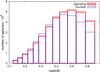Fig. 2 Redshift distribution of galaxies in the main lens samples (i.e. galaxies with redshifts 0.14 ≤ z ≤ 0.62, observer-frame r-band apparent magnitude mr ≤ 22.5, and stellar masses M ⋆  ≥ 109   h-1   M⊙) in the Garching and Durham model.

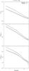Fig. 3 Aperture number count dispersion (top panel), (middle panel) and (bottom panel) measurements in the Garching model and Durham model.

For this sample of galaxies, the aperture number count dispersion  as a function of aperture radius is shown in the top panel of Fig. 3. The galaxy models clearly differ in the predicted dispersion: the Durham model predicts an up to two times larger amplitude than the Garching model. A similar difference has been observed for the angular galaxy correlation function by Kim et al. (2009), who attribute the discrepancy to too many bright satellites in the Durham model. However, as will be discussed below, the Garching model also appears to suffer from problems with the modeling of the satellite population.

The predictions for , shown in the middle panel of Fig. 3, exhibit fairly large differences between the models, too. The higher values of  in the Durham model, especially for smaller angular scales, imply more massive lens halos on average compared to the Garching model. The larger halo masses may also explain the higher clustering amplitude seen in . More massive halos host larger concentrations of galaxies and are themselves more clustered, which increases the correlation of the hosted galaxies on small and large scales. Another consequence is a larger third-order signal , which is confirmed by the bottom panel of Fig. 3.

4.2. Color-selected samples

For a further analysis, we divide the main lens galaxy samples into groups selected by color. From observations, the color distribution of galaxies is well characterized by a bimodal function (Strateva et al. 2001). At low redshifts, this can be approximated by the sum of two Gaussian functions representing red and blue subpopulations of galaxies on the red and blue side of the color distribution, respectively.

Following observations (e.g. Mandelbaum et al. 2006), we split the main lens galaxy samples at observer-frame color u − r = 2.2 to obtain subsamples of red and blue lens galaxies. For the Durham model, we obtain 2.4 × 10⁶ red and 6.1 × 10⁶ blue galaxies compared to 4 × 10⁶ red and 4.7 × 10⁶ blue galaxies in the Garching model. The redshift distributions of the color subsamples are shown in Fig. 4. The histograms show that the relative numbers of red and blue galaxies in each redshift bin differ significantly between the models.

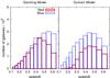Fig. 4 Number of red and blue galaxies in the Garching model and the Durham model. Red galaxies are selected to have u − r > 2.2 and blue galaxies are to have .

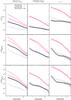Fig. 5 Aperture statistics for samples of red and blue galaxies in the Garching and Durham models. The left column shows the results for a fixed color-cut at u − r = 2.2 for galaxies with redshift between z = 0.14 and z = 0.62. The middle column displays the signals for galaxies between z = 0.14 and z = 0.62 separated using a redshift-dependent color cut. In the right column, galaxies are restricted to come from a single snapshot at redshift z = 0.17; accordingly error bars are larger.

The aperture statistics for these red and blue galaxy populations in both models are shown in the left panels of Fig. 5. In both models, red galaxies show higher signals than the blue galaxies. This trend is not surprising, since galaxies of different types follow different distribution patterns and clustering properties. Red galaxies are expected to be found mainly in groups and clusters associated with strong clustering and large halo masses, whereas blue galaxies are mostly field galaxies with smaller halos and lower clustering. The plot also shows that galaxies in the two models show different clustering statistics in both red and blue populations. This may be a result of selecting different objects in the models.

Studying the previous version of the Garching model based on the De Lucia & Blaizot (2007), Bett (2012) pointed out that the distributions of the observer-frame u − r colors are very different in the Garching model and the Durham model. In particular, galaxies appear redder in the Garching model than in the Durham model. We thus consider another way of dividing the galaxies into red and blue samples. We identify the minima of the bimodal distributions at each redshift. The positions of the minima are plotted in Fig. 6, clearly showing a large difference between the models in their color distribution. We then use the minima to separate red and blue galaxies.

Figure 7 shows the resulting redshift distributions of the red and blue subsamples. There are 4.2 × 10⁶ red and 4.3 × 10⁶ blue galaxies in the Durham model compared to 2.5 × 10⁶ red and 6.2 × 10⁶ blue galaxies in the Garching model. Now the difference between the models in the predicted numbers of red and blue galaxies is larger than for the case of a fixed color cut. This suggests that the redshift-dependent color cut selects very different objects in the two models. Surprisingly, the aperture statistics predicted by the two models are much more similar for the redshift-dependent color cuts than for the fixed color cut, as seen in the middle column of Fig. 5. The better agreement results from a decrease in the blue signals in the Durham model and an increase in the red signals in the Garching model.

The agreement between the two models shown in the middle column of Fig. 5 indicates that although the redshift distributions of red and blue galaxies differ, galaxies populate dark matter halos in such a way to produce similar results. This agreement between the models is more prominently seen in  and . Looking at , red Durham galaxies show a stronger signal on intermediate scales compared to the red Garching galaxies. This can happen, for example, if red galaxies in the Durham model are mostly central galaxies populating large massive halos. On the other hand, this difference may also be a result of the distinct redshift distributions. As will discussed this difference is not seen when galaxies are restricted to come from a single redshift.

Selecting lens galaxies at a single redshift amplifies the signal for  and  compared to a sample with a broad redshift distribution, where many of the projected galaxy pairs are at different redshifts and are therefore not correlated and suppress the overall signal. The third column of Fig. 5 displays the aperture measurements for lens galaxy populations selected from a single redshift slice around z = 0.17 with thickness Δz = 0.02. Now the signals for red galaxies agree well between the two models. The agreement is not so good for blue model galaxies, where the Garching model shows stronger signals on small and intermediate scales. In the halo-model language, blue Garching model galaxies at this redshift appear to live in more massive halos.

Both the Durham and the Garching models predict a larger ratio between the clustering strength of red and blue galaxies than has been obtained in observations. A similar behavior was seen when considering the previous incarnation of the Garching model based on De Lucia & Blaizot (2007). In particular, our results confirm the previous work of de la Torre et al. (2011), who compared the color-dependent projected two-point correlation function of a color subsample of galaxies in the VIMOS-VLT Deep Survey (VVDS; Le Fèvre et al. 2005) and in the model based on De Lucia & Blaizot (2007). They showed that red galaxies in the semi-analytic models have stronger clustering amplitudes than the observed ones. They linked this discrepancy to an overproduction of bright red galaxies in the model.

The different clustering strengths of red and blue galaxies show up very clearly in , , and . The ratio of the clustering amplitude of the red and blue samples is related to their relative bias (Sect. 2.3). This ratio can be measured based on different aperture statistics measurements presented in Fig. 5. Assuming a simple linear deterministic bias, the relative bias and its uncertainty is calculated on aperture scales of θ ~ 1   arcmin and θ ~ 10   arcmin in the Garching and Durham models. The results are shown in Table 1.

The differences in the bias ratios measured from different statistics point out that a linear deterministic bias model is not sufficient to describe the relation between the galaxy and matter distribution on different scales. This relation may be described by scale-dependent stochastic bias.

4.3. Magnitude-selected samples

In this section, we present the measurements of the second- and third-order aperture statistics for lens galaxies in six different bins of r-band absolute observer frame magnitude M_r. To eliminate effects of possibly different redshift distributions on the signals, we restrict the redshift range of the lens galaxy population to one redshift slice at z = 0.17. The results for all magnitude bins for the Garching (Durham) model are shown in the left (right) panels of Fig. 8.

There are common trends seen for both models in the second- and third-order aperture statistics. For the brighter bins ( − 23 ≤ M_r <  − 20), the aperture signals decrease rapidly with increasing magnitude M_r and filter scales θ. However, the Durham model predicts up to 200% higher , and  signals than the Garching model. Bright galaxies appear more clustered and on average to be located in more massive halos in the Durham model.

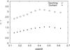Fig. 6 The u − r color-cut at each redshift in the Garching and Durham models.

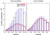Fig. 7 Number of red and blue galaxies counted in the Garching model and the Durham model. Galaxies at each redshift are selected according to the color-cut in Fig. 6.

For the fainter bins (−20 ≤ M_r <  −18), the signals increase with decreasing luminosity. This increase is contrary to observations of galaxy clustering and GGL (see e.g. McBride et al. 2011), where brighter galaxies show stronger clustering and larger lensing signals than fainter galaxies.

In the Garching model, the faint magnitude bins are over-populated with satellite galaxies, many of which have no own subhalo (this occurs when a galaxy has been stripped of its own halo during a merger process with a larger halo). These galaxies are abundant in massive halos, which contribute substantially to the  and  signal due to their large mass and stronger clustering. In the Durham model a similar trend is seen in  and , indicating similar problems with the modeling of the satellite population in massive halos.

The luminosity dependence of galaxy clustering has been studied extensively with the aid of galaxy surveys. Li et al. (2007) compared the luminosity dependence of the clustering of galaxies in the model of Croton et al. (2006) to results from the Sloan Digital Sky Survey Data Release Four (SDSS DR4; Adelman-McCarthy et al. 2006), and found that the faint model galaxies show a stronger clustering than SDSS galaxies.

Kim et al. (2009) compared the galaxy clustering predicted by the models of Bower et al. (2006), De Lucia & Blaizot (2007) and Font et al. (2008) to observed clustering in the two-degree Field Galaxy Redshift Survey (2dF, Colless et al. 2001). They found that none of the models are able to match the observed clustering properties of galaxies in different luminosity bins. In particular, the Durham model shows a stronger signal than expected, which could possibly be corrected, if the number of satellite galaxies in halos is reduced.

Both Li et al. (2007) and Kim et al. (2009) emphasize the problems of the galaxy models in predicting the luminosity dependence of galaxy clustering. Li et al. (2007) showed that the number of faint satellite galaxies has to be reduced by 30 per cent (regardless of their host halo mass) to better match the observed galaxy clustering. Kim et al. (2009) showed that the fraction of satellites declines with increasing luminosity (see, e.g. Fig. 4 in Kim et al. 2009) in the host halo mass range of 10¹²   h^-1   M_⊙ ≲ M_halo ≲ 10¹⁴   h^-1   M_⊙. Since the clustering strength depends strongly on the halo mass, satellite galaxies can affect the overall clustering amplitude. To investigate this they used a simple HOD model to show that satellite galaxies show a strong bias due to a strong two-halo clustering term. This indicates that satellite galaxies are preferentially found in massive halos which exhibits larger bias (see Fig. 5 in Kim et al. 2009). They argued that the results can be improved if the satellites are removed from massive halos by adding satellite-satellite merger processes in the models.

Our results suggest that the Garching model shows a similar problem with faint satellite galaxies, though to a lesser degree. Indeed, we find that the amplitude of the aperture signals in the faint bins are completely dominated by satellite galaxies in both the Durham and the Garching model. Most of these faint satellites reside in massive group and cluster halos, which results in very large aperture signals on the scales considered in this work.

5. Summary and discussion

Through observations of galaxy-galaxy(-galaxy) lensing, valuable information on the clustering properties of the galaxy and matter density field in the Universe can be obtained. Measurements of galaxy-galaxy lensing (GGL) can be used to infer information on the properties of dark matter halos hosting the lens galaxies (see, e.g., Schneider & Rix 1997; Johnston et al. 2007; Mandelbaum et al. 2008). Third-order galaxy lensing (G3L) can be used to infer information on the properties of a common dark matter halo hosting two lens galaxies (Simon et al. 2008, 2012).

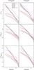Fig. 8 Aperture measurements in the Garching model (left panel) and the Durham model (right panel) in 6 different r-band absolute magnitude, Mr, bins.

In this work, we study how the information from GGL and G3L aperture statistics can be used to test models of galaxy formation and evolution. We investigate two semi-analytic galaxy formation models based on the Millennium Run N-body simulation of structure formation (Springel et al. 2005): the Durham model by Bower et al. (2006), and the Garching model by Guo et al. (2011). Using mock galaxy catalogs based on these models in conjunction with ray-tracing (Hilbert et al. 2009), we create simulated fields of galaxy lensing surveys. From these simulated surveys, we compute the model predictions for the second- and third-order aperture statistics , , and  for various galaxy populations.

We find that both semi-analytic models predict aperture signals that are qualitatively similar, but there are large quantitative differences. The Durham model predicts larger amplitudes for most considered galaxy samples. This indicates that lens galaxies in the Durham model tend to reside in more massive halos than lens galaxies in the Garching model.

In both the Durham and the Garching model, red galaxies exhibit stronger aperture signals than blue galaxies, in qualitative agreement with observations. However, both models predict a larger ratio between the clustering strength of red and blue galaxies than has been obtained in observations. These findings corroborate the findings of de la Torre et al. (2011), who showed that red galaxies in the semi-analytic models have stronger clustering amplitudes than red galaxies in observations. simulated data. We also argue that considering the amplitude ratio between the red and blue galaxies and making comparison between the second- and third-order aperture statistics leads to the conclusion that the third-order bias differs from the second-order bias. In other words, third-order aperture statistics provides new information which cannot be obtained from the second-order statistics alone. The large amplitude ratio between the clustering of red and blue galaxies in the models means a large relative bias of these galaxy populations. Measuring the biasing of galaxies provides information on the relative distribution of galaxies and the underlying matter distribution. We find that a linear deterministic bias model, even with scale-dependent bias parameters, is clearly ruled out by considering second and third-order aperture statistics for the simulated data. We expect that both statistics in combination will provide new information to constrain more advanced galaxy biasing models in the future.

In addition to the different prediction for red and blue galaxies, there are discrepancies between the predictions of the two models. For a fixed color cut at u − r = 2.2, the signals predicted by the Durham model are larger than those predicted by the Garching model. If a redshift-dependent color cut is used instead, the prediction from the two models for the aperture signals become more similar. However, the models then strongly disagree about the total numbers and redshift distributions of blue and red galaxies.

Both galaxy models predict that the aperture statistics decrease with decreasing luminosity for brighter galaxies in accordance with observations. However, the models also predict that the signals increase again for fainter galaxies. This behavior is most likely an artifact related to too many faint satellite galaxies in massive group and cluster halos predicted by the models. In fact, the fainter magnitude bins are completely dominated by satellite galaxies in both models. The problem appears more severe in the Durham model than in the Garching model, which differ in their treatment of satellite evolution.

We plan to extent our treatment in future work to study how well galaxy bias models with scale-dependent stochastic bias can be constrained with second- and third-order galaxy lensing statistics. One important question is how much information can be obtained from G3L in addition to that obtained from GGL.

Furthermore, we are looking forward to measurements of GGL and G3L signals in large ongoing and future surveys. The comparison of the observed signals and the signals predicted by galaxy models will help to identify shortcomings of the models and provide valuable hints for improvements in the models. This will also require a deeper understanding of the relation between the various details of the galaxy formation models and the predicted galaxy lensing and clustering signals.

Acknowledgments

We thank Phil Bett and Peder Norberg for helpful discussions. We thank the people of the Virgo Consortium for Cosmological Supercomputer Simulations and the German Astrophysical Virtual Observatory and all other people involved in making the Millennium Run simulation data and the galaxy catalogs of the semi-analytic galaxy formation models used in this work publicly available. This work was supported by the Deutsche Forschungsgemeinschaft (DFG) through the Priority Programme 1177 “Galaxy Evolution” (SCHN 342/6, SCHN 342/8–1, and WH 6/3) and through the Transregional Collaborative Research Centre TRR 33 “The Dark Universe”. S.H. also acknowledges support by the National Science Foundation (NSF) grant number AST-0807458-002.

References

Appendix A: Shot-noise correction

Assume a realization $({{\vartheta }}_{\mathit{i}}^{\mathrm{\left(}\mathit{r}\mathrm{\right)}})$, i = 1,...,N_g, of a set of N_g galaxies with sky positions ${{\vartheta }}_{\mathit{i}}^{\mathrm{\left(}\mathit{r}\mathrm{\right)}}$ in a field  with area A and mean galaxy number density of . Assume that each galaxy position is distributed in the field according to an underlying “true” number density field n_g(ϑ). The ensemble average of a quantity o(ϑ) over all realizations reads: $⟨\mathit{o}\left({\vartheta }\right)⟩\mathrm{=}\left[\underset{\mathit{k}\mathrm{=}\mathrm{1}}{\overset{{\mathit{N}}_{\mathrm{g}}}{\mathrm{􏽙}}}\frac{\mathrm{1}}{{\mathit{N}}_{\mathrm{g}}}{\mathrm{\int }}_{\mathrm{𝒜}}{\mathrm{d}}^{\mathrm{2}}{{\vartheta }}_{\mathit{k}}^{\mathrm{\left(}\mathit{r}\mathrm{\right)}}\hspace{0.17em}\mathit{n}\mathrm{(}{{{\vartheta }}_{\mathit{k}}^{\mathrm{\left(}\mathit{r}\mathrm{\right)}}}^{\mathrm{)}}\right]\mathit{o}\mathrm{\left(}{\vartheta }\mathrm{\right)}\mathit{.}$(A.1)For each realization, the random positions of the galaxies provide an estimate of the density field n_g: $\mathit{n̂}\begin{array}{}\mathrm{\left(}\mathit{r}\mathrm{\right)}\\ \mathrm{g}\end{array}\left({\vartheta }\right)\mathrm{=}\sum _{\mathit{i}\mathrm{=}\mathrm{1}}^{{\mathit{N}}_{\mathrm{g}}}{\mathit{\delta }}_{\mathrm{D}}\mathrm{(}{\vartheta }\mathrm{-}{{{\vartheta }}_{\mathit{i}}^{\mathrm{\left(}\mathit{r}\mathrm{\right)}}}^{\mathrm{)}}\mathit{.}$(A.2)This estimator is unbiased: $\begin{array}{ccc}\mathrm{⟨}{\mathit{n̂}\begin{array}{}\mathrm{\left(}\mathit{r}\mathrm{\right)}\\ \mathrm{g}\end{array}\left({\vartheta }\right)}^{\mathrm{⟩}}& \mathrm{=}& \left[\underset{\mathit{k}\mathrm{=}\mathrm{1}}{\overset{{\mathit{N}}_{\mathrm{g}}}{\mathrm{􏽙}}}\frac{\mathrm{1}}{{\mathit{N}}_{\mathrm{g}}}{\mathrm{\int }}_{\mathrm{𝒜}}{\mathrm{d}}^{\mathrm{2}}{{\vartheta }}_{\mathit{k}}^{\mathrm{\left(}\mathit{r}\mathrm{\right)}}\hspace{0.17em}{\mathit{n}}_{\mathrm{g}}\mathrm{(}{{{\vartheta }}_{\mathit{k}}^{\mathrm{\left(}\mathit{r}\mathrm{\right)}}}^{\mathrm{)}}\right]\sum _{\mathit{i}\mathrm{=}\mathrm{1}}^{{\mathit{N}}_{\mathrm{g}}}{\mathit{\delta }}_{\mathrm{D}}\mathrm{(}{\vartheta }\mathrm{-}{{{\vartheta }}_{\mathit{i}}^{\mathrm{\left(}\mathit{r}\mathrm{\right)}}}^{\mathrm{)}}\\ & \mathrm{=}& \sum _{\mathit{i}\mathrm{=}\mathrm{1}}^{{\mathit{N}}_{\mathrm{g}}}\left[\underset{\mathit{k}\mathrm{=}\mathrm{1}}{\overset{{\mathit{N}}_{\mathrm{g}}}{\mathrm{􏽙}}}\frac{\mathrm{1}}{{\mathit{N}}_{\mathrm{g}}}{\mathrm{\int }}_{\mathrm{𝒜}}{\mathrm{d}}^{\mathrm{2}}{{\vartheta }}_{\mathit{k}}^{\mathrm{\left(}\mathit{r}\mathrm{\right)}}\hspace{0.17em}{\mathit{n}}_{\mathrm{g}}\mathrm{(}{{{\vartheta }}_{\mathit{k}}^{\mathrm{\left(}\mathit{r}\mathrm{\right)}}}^{\mathrm{)}}\right]{\mathit{\delta }}_{\mathrm{D}}\mathrm{(}{\vartheta }\mathrm{-}{{{\vartheta }}_{\mathit{i}}^{\mathrm{\left(}\mathit{r}\mathrm{\right)}}}^{\mathrm{)}}\\ & \mathrm{=}& \sum _{\mathit{i}\mathrm{=}\mathrm{1}}^{{\mathit{N}}_{\mathrm{g}}}\frac{\mathrm{1}}{{\mathit{N}}_{\mathrm{g}}}{\mathrm{\int }}_{\mathrm{𝒜}}{\mathrm{d}}^{\mathrm{2}}{{\vartheta }}_{\mathit{i}}^{\mathrm{\left(}\mathit{r}\mathrm{\right)}}\hspace{0.17em}{\mathit{n}}_{\mathrm{g}}\mathrm{(}{{{\vartheta }}_{\mathit{i}}^{\mathrm{\left(}\mathit{r}\mathrm{\right)}}}^{\mathrm{)}}{\mathit{\delta }}_{\mathrm{D}}\mathrm{(}{\vartheta }\mathrm{-}{{{\vartheta }}_{\mathit{i}}^{\mathrm{\left(}\mathit{r}\mathrm{\right)}}}^{\mathrm{)}}\\ & \mathrm{=}& {\mathit{n}}_{\mathrm{g}}\left({\vartheta }\right)\mathit{.}\end{array}$(A.3)Using a filter function U(ϑ), we define a filtered density field  by: $\mathrm{𝒩}\left({\vartheta }\mathrm{;}\mathit{U}\right)\mathrm{=}{\mathrm{\int }}_{\mathrm{𝒜}}{\mathrm{d}}^{\mathrm{2}}{{\vartheta }}^{\mathrm{\prime }}\hspace{0.17em}\mathit{U}\left({\vartheta }\mathrm{-}{{\vartheta }}^{\mathrm{\prime }}\right)\hspace{0.17em}{\mathit{n}}_{\mathrm{g}}\left({{\vartheta }}^{\mathrm{\prime }}\right)\mathit{.}$(A.4)An estimator for the filtered field reads: $\mathrm{𝒩̂}\mathrm{\left(}\mathit{r}\mathrm{\right)}\left({\vartheta }\mathrm{;}\mathit{U}\right)\mathrm{=}{\mathrm{\int }}_{\mathrm{𝒜}}{\mathrm{d}}^{\mathrm{2}}{{\vartheta }}^{\mathrm{\prime }}\hspace{0.17em}\mathit{U}\left({\vartheta }\mathrm{-}{{\vartheta }}^{\mathrm{\prime }}\right)\hspace{0.17em}\mathit{n̂}\begin{array}{}\mathrm{\left(}\mathit{r}\mathrm{\right)}\\ \mathrm{g}\end{array}\left({{\vartheta }}^{\mathrm{\prime }}\right)\mathrm{=}\sum _{\mathit{i}\mathrm{=}\mathrm{1}}^{{\mathit{N}}_{\mathrm{g}}}\mathit{U}\mathrm{(}{\vartheta }\mathrm{-}{{{\vartheta }}_{\mathit{i}}^{\mathrm{\left(}\mathit{r}\mathrm{\right)}}}^{\mathrm{)}}\mathit{.}$(A.5)Its expectation value $\begin{array}{ccc}{\mathrm{⟨}\mathrm{𝒩̂}\mathrm{\left(}\mathit{r}\mathrm{\right)}{\left({\vartheta }\mathrm{;}\mathit{U}\right)}^{\mathrm{⟩}}}_{\mathit{r}}& \mathrm{=}& \left[\underset{\mathit{k}\mathrm{=}\mathrm{1}}{\overset{{\mathit{N}}_{\mathrm{g}}}{\mathrm{􏽙}}}\frac{\mathrm{1}}{{\mathit{N}}_{\mathrm{g}}}{\mathrm{\int }}_{\mathrm{𝒜}}{\mathrm{d}}^{\mathrm{2}}{{\vartheta }}_{\mathit{k}}^{\mathrm{\left(}\mathit{r}\mathrm{\right)}}\hspace{0.17em}{\mathit{n}}_{\mathrm{g}}\mathrm{(}{{{\vartheta }}_{\mathit{k}}^{\mathrm{\left(}\mathit{r}\mathrm{\right)}}}^{\mathrm{)}}\right]\sum _{\mathit{i}\mathrm{=}\mathrm{1}}^{{\mathit{N}}_{\mathrm{g}}}\mathit{U}\mathrm{(}{\vartheta }\mathrm{-}{{{\vartheta }}_{\mathit{i}}^{\mathrm{\left(}\mathit{r}\mathrm{\right)}}}^{\mathrm{)}}\\ & \mathrm{=}& \sum _{\mathit{i}\mathrm{=}\mathrm{1}}^{{\mathit{N}}_{\mathrm{g}}}\frac{\mathrm{1}}{{\mathit{N}}_{\mathrm{g}}}{\mathrm{\int }}_{\mathrm{𝒜}}{\mathrm{d}}^{\mathrm{2}}{{\vartheta }}_{\mathit{i}}^{\mathrm{\left(}\mathit{r}\mathrm{\right)}}\hspace{0.17em}{\mathit{n}}_{\mathrm{g}}\mathrm{(}{{{\vartheta }}_{\mathit{i}}^{\mathrm{\left(}\mathit{r}\mathrm{\right)}}}^{\mathrm{)}}\mathit{U}\mathrm{(}{\vartheta }\mathrm{-}{{{\vartheta }}_{\mathit{i}}^{\mathrm{\left(}\mathit{r}\mathrm{\right)}}}^{\mathrm{)}}\\ & \mathrm{=}& \int \mathrm{𝒜}{\mathrm{d}}^{\mathrm{2}}{{\vartheta }}^{\mathrm{\prime }}\hspace{0.17em}{\mathit{n}}_{\mathrm{g}}\left({{\vartheta }}^{\mathrm{\prime }}\right)\mathit{U}\left({\vartheta }\mathrm{-}{{\vartheta }}^{\mathrm{\prime }}\right)\\ & \mathrm{=}& \mathrm{𝒩}\left({\vartheta }\mathrm{;}\mathit{U}\right)\mathit{.}\end{array}$(A.6)Consider the square of the filtered density $\begin{array}{ccc}{\mathrm{𝒩}}^{\mathrm{2}}\left({\vartheta }\mathrm{;}\mathit{U}\right)& \mathrm{=}& \int \mathrm{𝒜}{\mathrm{d}}^{\mathrm{2}}{{\vartheta }}^{\mathrm{\prime }}{\mathrm{\int }}_{\mathrm{𝒜}}{\mathrm{d}}^{\mathrm{2}}{{\vartheta }}^{\mathrm{\prime \prime }}\hspace{0.17em}\mathit{U}\left({\vartheta }\mathrm{-}{{\vartheta }}^{\mathrm{\prime }}\right)\hspace{0.17em}\mathit{U}\left({\vartheta }\mathrm{-}{{\vartheta }}^{\mathrm{\prime \prime }}\right)\\ & & \mathrm{\times }{\mathit{n}}_{\mathrm{g}}\left({{\vartheta }}^{\mathrm{\prime }}\right)\hspace{0.17em}{\mathit{n}}_{\mathrm{g}}\left({{\vartheta }}^{\mathrm{\prime \prime }}\right)\mathit{.}\end{array}$(A.7)A naive estimator is provided by: $\begin{array}{ccc}\mathrm{⟨}{[\mathrm{𝒩̂}\mathrm{\left(}\mathit{r}\mathrm{\right)}\left({\vartheta }\mathrm{;}\mathit{U}\right){]}^{\mathrm{2}}}^{\mathrm{⟩}}& \mathrm{=}& \left[\underset{\mathit{k}\mathrm{=}\mathrm{1}}{\overset{{\mathit{N}}_{\mathrm{g}}}{\mathrm{􏽙}}}\frac{\mathrm{1}}{{\mathit{N}}_{\mathrm{g}}}{\mathrm{\int }}_{\mathrm{𝒜}}{\mathrm{d}}^{\mathrm{2}}{{\vartheta }}_{\mathit{k}}^{\mathrm{\left(}\mathit{r}\mathrm{\right)}}\hspace{0.17em}{\mathit{n}}_{\mathrm{g}}\mathrm{(}{{{\vartheta }}_{\mathit{k}}^{\mathrm{\left(}\mathit{r}\mathrm{\right)}}}^{\mathrm{)}}\right]\\ & & \mathrm{\times }\sum _{\mathit{i}\mathrm{=}\mathrm{1}}^{{\mathit{N}}_{\mathrm{g}}}\mathit{U}\mathrm{(}{\vartheta }\mathrm{-}{{{\vartheta }}_{\mathit{i}}^{\mathrm{\left(}\mathit{r}\mathrm{\right)}}}^{\mathrm{)}}\sum _{\mathit{j}\mathrm{=}\mathrm{1}}^{{\mathit{N}}_{\mathrm{g}}}\mathit{U}\left({\vartheta }\mathrm{-}{{\vartheta }}_{\mathit{j}}^{\mathrm{\left(}\mathit{r}\mathrm{\right)}}\right)\\ & \mathrm{=}& \begin{array}{}{\mathit{N}}_{\mathrm{g}}\\ \sum \\ \mathit{i}\ne \mathit{j}\mathit{i,j}\mathrm{=}\mathrm{1}\end{array}\frac{\mathrm{1}}{{\mathit{N}}_{\mathrm{g}}^{\mathrm{2}}}{\mathrm{\int }}_{\mathrm{𝒜}}{\mathrm{d}}^{\mathrm{2}}{{\vartheta }}_{\mathit{i}}^{\mathrm{\left(}\mathit{r}\mathrm{\right)}}{\mathrm{\int }}_{\mathrm{𝒜}}{\mathrm{d}}^{\mathrm{2}}{{\vartheta }}_{\mathit{j}}^{\mathrm{\left(}\mathit{r}\mathrm{\right)}}\hspace{0.17em}{\mathit{n}}_{\mathrm{g}}\mathrm{(}{{{\vartheta }}_{\mathit{i}}^{\mathrm{\left(}\mathit{r}\mathrm{\right)}}}^{\mathrm{)}}\hspace{0.17em}{\mathit{n}}_{\mathrm{g}}\left({{\vartheta }}_{\mathit{j}}^{\mathrm{\left(}\mathit{r}\mathrm{\right)}}\right)\\ & & \mathrm{\times }\mathit{U}\mathrm{(}{\vartheta }\mathrm{-}{{{\vartheta }}_{\mathit{i}}^{\mathrm{\left(}\mathit{r}\mathrm{\right)}}}^{\mathrm{)}}\hspace{0.17em}\mathit{U}\left({\vartheta }\mathrm{-}{{\vartheta }}_{\mathit{j}}^{\mathrm{\left(}\mathit{r}\mathrm{\right)}}\right)\\ & & \mathrm{+}\sum _{\mathit{i}\mathrm{=}\mathrm{1}}^{{\mathit{N}}_{\mathrm{g}}}\frac{\mathrm{1}}{{\mathit{N}}_{\mathrm{g}}}{\mathrm{\int }}_{\mathrm{𝒜}}{\mathrm{d}}^{\mathrm{2}}{{\vartheta }}_{\mathit{i}}^{\mathrm{\left(}\mathit{r}\mathrm{\right)}}\hspace{0.17em}{\mathit{n}}_{\mathrm{g}}\mathrm{(}{{{\vartheta }}_{\mathit{i}}^{\mathrm{\left(}\mathit{r}\mathrm{\right)}}}^{\mathrm{)}}\mathit{U}{\mathrm{(}{\vartheta }\mathrm{-}{{{\vartheta }}_{\mathit{i}}^{\mathrm{\left(}\mathit{r}\mathrm{\right)}}}^{\mathrm{)}}}^{\mathrm{2}}\\ & \mathrm{=}& \end{array}$(A.8)Hence, this estimator is biased. The first term of the last line is actually what is intended to be measured as aperture dispersion (up to a prefactor close to unity). The second term is due to shot noise arising from the Poisson sampling of the density field. An unbiased estimator of  is provided by $\begin{array}{ccc}& & \frac{{\mathit{N}}_{\mathrm{g}}}{{\mathit{N}}_{\mathrm{g}}\mathrm{-}\mathrm{1}}\left\{[\mathrm{𝒩̂}\mathrm{\left(}\mathit{r}\mathrm{\right)}\left({\vartheta }\mathrm{;}\mathit{U}\right){]}^{\mathrm{2}}\mathrm{-}\mathrm{𝒩̂}\mathrm{\left(}\mathit{r}\mathrm{\right)}\mathrm{(}{\vartheta }\mathrm{;}{\mathit{U}}^{\mathrm{2}}\mathrm{)}\right\}\mathrm{=}\frac{{\mathit{N}}_{\mathrm{g}}}{{\mathit{N}}_{\mathrm{g}}\mathrm{-}\mathrm{1}}\\ & & \mathrm{\times }\begin{array}{}{\mathit{N}}_{\mathrm{g}}\\ \sum \\ \mathit{i}\ne \mathit{j}\mathit{i,j}\mathrm{=}\mathrm{1}\end{array}\mathit{U}\mathrm{(}{\vartheta }\mathrm{-}{{{\vartheta }}_{\mathit{i}}^{\mathrm{\left(}\mathit{r}\mathrm{\right)}}}^{\mathrm{)}}\mathit{U}\left({\vartheta }\mathrm{-}{{\vartheta }}_{\mathit{j}}^{\mathrm{\left(}\mathit{r}\mathrm{\right)}}\right)\mathit{.}\end{array}$(A.9)By projecting the galaxy positions of a realization onto a mesh (e.g. using Nearest-Grid-Point assignment), one obtains a discretized representation of the density estimate (A.2). The density

estimate on the mesh can then be convolved, e.g. by using FFTs, with the filters U and U² to obtain gridded versions of the unbiased estimates for  and . The latter estimate can then be subtracted point-wise from the square of the former estimate to calculate the unbiased estimate (A.9).

All Tables

All Figures

Fig. 1 Upper panel: aperture statistics as a function of filter scale θ measured in the Garching model. The FFT method (squares) and the tree method (triangles) are compared for lenses at redshift z = 0.17 with mr ≤ 22.5, stellar masses M⋆ ≥ 109   h-1   M⊙ and convergence field of sources at redshift z = 0.99. Error bars indicate the standard deviation of for aperture radius θ estimated across 32 fields. Lower panel: average difference signal between the FFT method and the tree method. Again the error bars show the standard deviation of the mean (field variance of difference signal divided by $\sqrt{\mathrm{31}}$).

In the text

	Fig. 2 Redshift distribution of galaxies in the main lens samples (i.e. galaxies with redshifts 0.14 ≤ z ≤ 0.62, observer-frame r-band apparent magnitude mr ≤ 22.5, and stellar masses M ⋆  ≥ 109   h-1   M⊙) in the Garching and Durham model.
In the text

	Fig. 3 Aperture number count dispersion (top panel), (middle panel) and (bottom panel) measurements in the Garching model and Durham model.
In the text

	Fig. 4 Number of red and blue galaxies in the Garching model and the Durham model. Red galaxies are selected to have u − r > 2.2 and blue galaxies are to have .
In the text

Fig. 5 Aperture statistics for samples of red and blue galaxies in the Garching and Durham models. The left column shows the results for a fixed color-cut at u − r = 2.2 for galaxies with redshift between z = 0.14 and z = 0.62. The middle column displays the signals for galaxies between z = 0.14 and z = 0.62 separated using a redshift-dependent color cut. In the right column, galaxies are restricted to come from a single snapshot at redshift z = 0.17; accordingly error bars are larger.

In the text

	Fig. 6 The u − r color-cut at each redshift in the Garching and Durham models.
In the text

	Fig. 7 Number of red and blue galaxies counted in the Garching model and the Durham model. Galaxies at each redshift are selected according to the color-cut in Fig. 6.
In the text

	Fig. 8 Aperture measurements in the Garching model (left panel) and the Durham model (right panel) in 6 different r-band absolute magnitude, Mr, bins.
In the text

References

- Adelman-McCarthy, J. K., Agüeros, M. A., Allam, S. S., et al. 2006, ApJS, 162, 38 [NASA ADS] [CrossRef] [Google Scholar]
- Bardeen, J. M., Bond, J. R., Kaiser, N., & Szalay, A. S. 1986, ApJ, 304, 15 [NASA ADS] [CrossRef] [Google Scholar]
- Bartelmann, M., & Schneider, P. 2001, Phys. Rep., 340, 291 [NASA ADS] [CrossRef] [Google Scholar]
- Bett, P. 2012, MNRAS, 420, 3303 [NASA ADS] [CrossRef] [Google Scholar]
- Bower, R. G., Benson, A. J., Malbon, R., et al. 2006, MNRAS, 370, 645 [NASA ADS] [CrossRef] [Google Scholar]
- Brainerd, T. G., Blandford, R. D., & Smail, I. 1996, ApJ, 466, 623 [NASA ADS] [CrossRef] [Google Scholar]
- Colless, M., Dalton, G., Maddox, S., et al. 2001, MNRAS, 328, 1039 [NASA ADS] [CrossRef] [Google Scholar]
- Cooray, A., & Sheth, R. 2002, Phys. Rep., 372, 1 [NASA ADS] [CrossRef] [Google Scholar]
- Crittenden, R. G., Natarajan, P., Pen, U.-L., & Theuns, T. 2002, ApJ, 568, 20 [NASA ADS] [CrossRef] [Google Scholar]
- Croton, D. J., Springel, V., White, S. D. M., et al. 2006, MNRAS, 365, 11 [NASA ADS] [CrossRef] [Google Scholar]
- de la Torre, S., Meneux, B., De Lucia, G., et al. 2011, A&A, 525, A125 [NASA ADS] [CrossRef] [EDP Sciences] [Google Scholar]
- De Lucia, G., & Blaizot, J. 2007, MNRAS, 375, 2 [NASA ADS] [CrossRef] [Google Scholar]
- Dekel, A., & Lahav, O. 1999, ApJ, 520, 24 [NASA ADS] [CrossRef] [MathSciNet] [Google Scholar]
- Font, A. S., Bower, R. G., McCarthy, I. G., et al. 2008, MNRAS, 389, 1619 [NASA ADS] [CrossRef] [Google Scholar]
- Frigo, M., & Johnson, S. G. 2005, Proc. IEEE, 93, 216, invited paper, special issue on The Design and Implementation of FFTW3 [Google Scholar]
- Gladders, M. D., & Yee, H. K. C. 2005, ApJS, 157, 1 [NASA ADS] [CrossRef] [Google Scholar]
- Guo, Q., White, S., Boylan-Kolchin, M., et al. 2011, MNRAS, 413, 101 [NASA ADS] [CrossRef] [Google Scholar]
- Hilbert, S., Hartlap, J., White, S. D. M., & Schneider, P. 2009, A&A, 499, 31 [NASA ADS] [CrossRef] [EDP Sciences] [Google Scholar]
- Hoekstra, H., van Waerbeke, L., Gladders, M. D., Mellier, Y., & Yee, H. K. C. 2002, ApJ, 577, 604 [NASA ADS] [CrossRef] [Google Scholar]
- Johnston, D. E., Sheldon, E. S., Wechsler, R. H., et al. 2007 [arXiv:0709.1159] [Google Scholar]
- Jullo, E., Rhodes, J., Kiessling, A., et al. 2012, ApJ, 750, 37 [NASA ADS] [CrossRef] [Google Scholar]
- Kaiser, N. 1984, ApJ, 284, L9 [NASA ADS] [CrossRef] [Google Scholar]
- Kauffmann, G., Colberg, J. M., Diaferio, A., & White, S. D. M. 1999, MNRAS, 303, 188 [NASA ADS] [CrossRef] [Google Scholar]
- Kim, H.-S., Baugh, C. M., Cole, S., Frenk, C. S., & Benson, A. J. 2009, MNRAS, 400, 1527 [NASA ADS] [CrossRef] [Google Scholar]
- Kleinheinrich, M., Schneider, P., Rix, H.-W., et al. 2006, A&A, 455, 441 [NASA ADS] [CrossRef] [EDP Sciences] [Google Scholar]
- Le Fèvre, O., Vettolani, G., Garilli, B., et al. 2005, A&A, 439, 845 [NASA ADS] [CrossRef] [EDP Sciences] [Google Scholar]
- Lemson, G., & Virgo Consortium, T. 2006 [arXiv:0608019] [Google Scholar]
- Li, C., Jing, Y. P., Kauffmann, G., et al. 2007, MNRAS, 376, 984 [NASA ADS] [CrossRef] [Google Scholar]
- Mandelbaum, R., Hirata, C. M., Broderick, T., Seljak, U., & Brinkmann, J. 2006, MNRAS, 370, 1008 [NASA ADS] [CrossRef] [Google Scholar]
- Mandelbaum, R., Seljak, U., & Hirata, C. M. 2008, J. Cosmology Astropart. Phys., 8, 6 [Google Scholar]
- McBride, C. K., Connolly, A. J., Gardner, J. P., et al. 2011, ApJ, 726, 13 [NASA ADS] [CrossRef] [Google Scholar]
- Mo, H. J., Jing, Y. P., & White, S. D. M. 1996, MNRAS, 282, 1096 [NASA ADS] [CrossRef] [Google Scholar]
- Schneider, P. 1996, MNRAS, 283, 837 [NASA ADS] [CrossRef] [Google Scholar]
- Schneider, P. 1998, ApJ, 498, 43 [NASA ADS] [CrossRef] [Google Scholar]
- Schneider, P., & Rix, H.-W. 1997, ApJ, 474, 25 [NASA ADS] [CrossRef] [Google Scholar]
- Schneider, P., & Watts, P. 2005, A&A, 432, 783 [NASA ADS] [CrossRef] [EDP Sciences] [Google Scholar]
- Schneider, P., van Waerbeke, L., Jain, B., & Kruse, G. 1998, MNRAS, 296, 873 [NASA ADS] [CrossRef] [Google Scholar]
- Schneider, P., Kochanek, C., & Wambsganss, J. 2006, Gravitational lensing: strong, weak and micro, Saas-Fee Advanced Course: Swiss Society for Astrophysics and Astronomy (Springer) [Google Scholar]
- Simon, P., Hetterscheidt, M., Schirmer, M., et al. 2007, A&A, 461, 861 [NASA ADS] [CrossRef] [EDP Sciences] [Google Scholar]
- Simon, P., Watts, P., Schneider, P., et al. 2008, A&A, 479, 655 [NASA ADS] [CrossRef] [EDP Sciences] [Google Scholar]
- Simon, P., Schneider, P., & Kübler, D. 2012, A&A, in press, DOI: 10.1051/0004-6361/201218993 [Google Scholar]
- Springel, V., White, S. D. M., Tormen, G., & Kauffmann, G. 2001, MNRAS, 328, 726 [Google Scholar]
- Springel, V., White, S. D. M., Jenkins, A., et al. 2005, Nature, 435, 629 [NASA ADS] [CrossRef] [PubMed] [Google Scholar]
- Strateva, I., Ivezić, Ž., Knapp, G. R., et al. 2001, AJ, 122, 1861 [Google Scholar]
- van Uitert, E., Hoekstra, H., Velander, M., et al. 2011, A&A, 534, A14 [NASA ADS] [CrossRef] [EDP Sciences] [Google Scholar]
- van Waerbeke, L. 1998, A&A, 334, 1 [NASA ADS] [Google Scholar]
- White, S. D. M., & Frenk, C. S. 1991, ApJ, 379, 52 [NASA ADS] [CrossRef] [Google Scholar]