| Issue |
A&A
Volume 547, November 2012
|
|
|---|---|---|
| Article Number | A34 | |
| Number of page(s) | 12 | |
| Section | The Sun | |
| DOI | https://doi.org/10.1051/0004-6361/201219272 | |
| Published online | 24 October 2012 | |
Unusual Stokes V profiles during flaring activity of a delta sunspot
1
ESA/ESTEC RSSD, Keplerlaan 1,
2200 AG
Noordwijk,
The Netherlands
e-mail: This email address is being protected from spambots. You need JavaScript enabled to view it.
2
Sterrewacht Leiden, Universiteit Leiden,
Niels Bohrweg 2, 2333 CA
Leiden, The
Netherlands
3
School of Physics and Astronomy, SUPA, University of
Glasgow, Glasgow
G12 8QQ,
UK
4
Instituto de Astrofísica de Canarias, Avda Vía Láctea S/N, La Laguna 38200,
Tenerife,
Spain
Received: 23 March 2012
Accepted: 4 September 2012
Abstract
Aims. We analyze a set of full Stokes profile observations of the flaring active region NOAA 10808. The region was recorded with the Vector-Spectromagnetograph of the Synoptic Optical Long-term Investigations of the Sun facility. The active region produced several successive X-class flares between 19:00 UT and 24:00 UT on September 13, 2005 and we aim to quantify transient and permanent changes in the magnetic field and velocity field during one of the flares, which has been fully captured.
Methods. The Stokes profiles were inverted using the height-dependent inversion code LILIA to analyze magnetic field vector changes at the flaring site. We report multilobed asymmetric Stokes V profiles found in the δ-sunspot umbra. We fit the asymmetric Stokes V profiles assuming an atmosphere consisting of two components (SIR inversions) to interpret the profile shape. The results are put in context with Michelson Doppler Imager (MDI) magnetograms and reconstructed X-ray images from the Reuven Ramaty High Energy Solar Spectroscopic Imager.
Results. We obtain the magnetic field vector and find signs of restructuring of the photospheric magnetic field during the flare close to the polarity inversion line at the flaring site. At two locations in the umbra we encounter strong fields (~3 kG), as inferred from the Stokes I profiles, which, however, exhibit a low polarization signal. During the flare we observe in addition asymmetric Stokes V profiles at one of these sites. The asymmetric Stokes V profiles appear co-spatial and co-temporal with a strong apparent polarity reversal observed in MDI-magnetograms and a chromospheric hard X-ray source. The two-component atmosphere fits of the asymmetric Stokes profiles result in line-of-sight velocity differences in the range of ~12 km s-1 to 14 km s-1 between the two components in the photosphere. Another possibility is that local atmospheric heating is causing the observed asymmetric Stokes V profile shape. In either case our analysis shows that a very localized patch of ~5″ in the photospheric umbra, co-spatial with a flare footpoint, exhibits a subresolution fine structure.
Key words: sunspots / Sun: photosphere / Sun: flares / Sun: surface magnetism
© ESO, 2012
1. Introduction
It is generally believed that flares are the result of the release of stored magnetic energy during a reconnection process accompanied by a change of the magnetic topology (see e.g. Carmichael 1964; Sturrock & Coppi 1966; Kopp & Pneuman 1976). Photospheric magnetic shear and disturbance of already emerged magnetic loops by new flux emergence are suspected to play an important role in the energy loading process, see e.g., Kusano et al. (2002), Engell et al. (2011) or the recent review by Shibata & Magara (2011).
The back reaction of a strong energy release on the lower atmosphere has been observed as photospheric “sunquake” (Kosovichev & Zharkova 1998; Donea & Lindsey 2005), non-reversing changes in the line-of-sight magnetic field (Cameron & Sammis 1999; Sudol & Harvey 2005), and heating of the chromospheric temperature minimum and upper photosphere (Machado & Rust 1974; Metcalf et al. 1990; Xu et al. 2004). It is clear that the effects of the enormous, yet localized, release of stored magnetic energy in the corona has dramatic impacts on the atmosphere beneath, but the manner of the observed response of the deep atmosphere remains a puzzle. The primary agents for carrying energy in flares are thought to be fast electrons, but these cannot penetrate deep enough into the atmosphere, in sufficient numbers, to directly generate the observed heating (Aboudarham & Henoux 1986). Fast ions have a farther penetration range, but though these are almost certain to exist in large numbers in flares, they are difficult to observe. In any case both sunquakes and chromospheric/photospheric heating seem to be closer associated with electrons (Fletcher et al. 2007; Kosovichev 2007). Heating of the mid- or upper chromosphere resulting in the emission of UV radiation that then causes photospheric “backwarming” (Machado et al. 1989) is also likely. Energy may also be carried by magnetic disturbances, which have the potential to penetrate deep into the atmosphere (Fletcher & Hudson 2008), but their dissipation and heating is as yet unknown.
One of the major obstacles in studying the connection of photospheric magnetic footpoints and flare events is the lack of observations of the full magnetic vector in the lower photosphere during a flare. So far, only a few full Stokes profile measurements were recorded covering a flare e.g., Hirzberger et al. (2009, Swedish Solar Telescope), Kubo et al. (2007, Hinode), and recently Wang et al. (2012, Solar Dynamics Observatory, SDO). Covering a larger flare site as is often required in M- and X-class flares comes at the expense of either spatial, spectral or temporal resolution. Only with sufficient spectral sampling in the Stokes profiles can one infer subresolution structures or draw conclusions on strong gradients in the atmospheric parameters from the shape of the profiles (Frutiger & Solanki 1998; Sigwarth 2001; Müller et al. 2006; Viticchié & Sánchez Almeida 2011). For example, Kleint (2012) revealed a complex multicomponent atmosphere around flare footpoints by analyzing high-resolution Interferometric BIdimensional Spectrometer (IBIS) data.
 |
Fig. 1 Active region NOAA 10808 on September 13, 2005. Left: magnetogram obtained from SOLIS-VSM Stokes V profile amplitudes in the Fe i 630.25 nm line. The white areas denote positive magnetic flux, while the black areas are regions exhibiting negative magnetic flux. The orange line shows the intricate polarity inversion line (PIL). Right: co-spatial intensity image constructed from the Stokes I continuum intensities. |
The rare full Stokes data set presented here gives us the opportunity to investigate the magnetic field vector changes associated with a flare, but due to the high spectral resolution also allows a more detailed analysis of the Stokes profile shapes. This offers the possibility of understanding not only the flare magnetic field evolution at the photospheric level, but also heating and flows in the deep atmosphere.
The observed active region, NOAA 10808, showed a complex structure and is a so-called δ-spot, because its two opposite polarity umbrae share a common penumbra. Figure 1 shows the magnetogram and the continuum intensity of the active region. The intricate polarity inversion line (PIL) indicates the high complexity of the magnetic configuration that is typical for a δ-sunspot. NOAA 10808 displayed a high flare activity, producing over ten X-class flares and many M-class and C-class flares during its presence on the observable solar disk. On September 13, 2005 the active region was located almost at the center of the solar disk and the Geostationary Operational Environmental Satellites (GOES) recorded a succession of soft X-ray (SXR) flux peaks within 4.5 h. Figure 2 shows the SXR flux registered by GOES and indicates the SOLIS (Synoptic Optical Long-term Investigations of the Sun) Vector-Spectromagnetograph (VSM) observation time, as well as the observation time of RHESSI (Reuven Ramaty High Energy Solar Spectroscopic Imager). Michelson Doppler Imager (MDI) magnetograms are available for the entire time section. The flare numbering is adopted from Liu et al. (2009), who analyzed the flares i–iv using a wide range of wavelength bands. These authors were particularly interested in the evolution of successive flares and concluded that the events were interconnected. Liu and collaborators identified the delta spot umbra as the location of flare iii. They support their view by analyzing RHESSI hard X-ray (HXR) reconstructed images. Flare ii cannot be identified in the GOES SXR flux. However, Wang et al. (2007) observed a clear flare signature of two Hα kernels moving apart associated with a filament eruption. There have been in addition several studies of the individual flares by e.g., Nagashima et al. (2007), Chifor et al. (2007), and Canou et al. (2009) as well as comparisons with simulations of the large-scale emergence of a twisted flux rope (Archontis & Hood 2010).
2. Observations
2.1. Data reduction
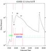 |
Fig. 2 GOES X-ray flux recorded on September 13, 2005. The flare numbers, adapted from Liu et al. (2009), are indicated with capital roman numbers. The second flare is not discernible in the soft X-ray flux. The SOLIS-VSM observation time from 19:36 UT to 20:57 UT is represented by the red solid line. MDI, recording magnetograms in Ni i 676.77 nm, and the RHESSI observing times are indicated with green dashed-dotted and blue dashed lines, respectively. |
The Stokes profiles were recorded with the ground-based SOLIS Vector-Spectromagnetograph (Keller & SOLIS Team 2003) on September 13, 2005. The SOLIS-VSM has a polarization sensitivity of a few 10-4 per pixel in less than one second and is capable of obtaining the full Stokes profiles for a limb-to-limb slice of ~337″ in width at a cadence of 5 min. The scans were performed by slit scanning with the slit positioned in the geocentric west-east direction and a stepwidth of 1.125″. The pixel size is 1.125″ and the spectral window encompasses the two Fe i lines at 630.15 nm and 630.25 nm with a resolution of 0.0027 nm per pixel. The dark currents were subtracted from the raw data and a flat-field correction was employed. The polarization demodulation matrix was applied to obtain Stokes I, Q, U, and V and fringes were removed. All profiles were normalized to the continuum of the quiet-Sun intensity, which was obtained by averaging the continuum values of ten quiet Sun pixel positions around disk center. We correlated the magnetograms thus obtained to counteract the spatial drift present between successive active region scans. Unfortunately, the measurement of the polarized spectrum was in some parts severely affected by the deterioration of the polarization modulator. The ferro-electric liquid crystal (FLC) polarization modulator package is located behind the entrance slit. The deteriorating effect of the FLC is the not uncommon formation of limited areas that do not show the expected half-wave retardation and/or fast axis orientation change. While the polarization calibration corrects for these effects, it cannot compensate for the loss in polarimetric efficiency. Therefore, the retrieved Stokes vector in the affected areas is still correct, but the noise is amplified dramatically. Because the FLC is close to the entrance slit, the affected area is also limited in the spatial direction along the slit. The profiles in these regions (eastern part of the active region) remained noisy throughout the time sequence. Fortunately, large parts of the umbra of the δ-spot are unaffected.
2.2. Inversion of the entire region
We used the inversion code LILIA (Socas-Navarro 2001), which is based on the Levenberg-Marquardt algorithm, to perform the inversions and obtain the global magnetic field vector map. LILIA assumes local thermodynamic equilibrium and uses a height-dependent model with temperature, microturbulence, macroturbulence, magnetic field strength, line-of-sight velocity, magnetic inclination, and magnetic azimuth as the atmospheric fit parameters. A (non-polarized) stray-light profile can be provided to the code. This profile can represent the contribution of a nonmagnetic atmospheric component in the resolution element or/and instrumental stray-light contaminating the observation. The code then determines a filling factor of this stray-light profile, which we refer to throughout as the stray-light factor. We used the averaged Stokes I profile of ten quiet Sun pixels located close to the active region as the stray-light profile. Semi-empirical models obtained by Socas-Navarro (2007) were used as initial model atmospheres for the umbra, penumbra, and plage profiles, respectively. We applied the nonpotential magnetic field calculation method of Georgoulis (2005) to resolve the 180° disambiguation in the azimuth angle of the magnetic field vector. In this code the vertical electric current Jz is iteratively minimized. We used Jz retrieved from the disambiguation of the first time scan as an initial proxy for Jz in the following time step and carried on in this way, always using the previous values for the initialization, to guarantee consistency between the time steps.
2.3. Asymmetric profile fits
Because LILIA uses a height-dependent model atmosphere, it goes beyond Milne-Eddington inversions (Skumanich & Lites 1987) and is therefore theoretically able to fit asymmetries in the Stokes V profiles. However, it uses only one magnetic atmospheric component and therefore the complicated profiles caused by superposition of shifted profiles and opposite polarity components in a single spatial resolution element cannot be fitted. The SIR code (Bellot Rubio 2003; Ruiz Cobo & del Toro Iniesta 1992) is capable of using two magnetic components as well as an additional stray-light component, and we employed it to invert the multilobed asymmetric profiles. We were unable, however, to achieve a satisfactory fit for all asymmetric profiles. For these remaining cases we therefore did not perform an inversion and used instead a simple approach by constructing anti-symmetric Stokes V profiles consisting of two Gaussians with opposite signs. We allowed the synthetic anti-symmetric Stokes V profiles to be shifted with respect to each other and to carry an optional sign reversal and vary their line width and amplitude. We used these parameters in a fitting routine employing nonlinear least squares minimization to determine the best fit to the observed asymmetric Stokes V profiles.
 |
Fig. 3 RHESSI light curves on September 13, 2005. The light curves were corrected for attenuator and decimation state changes. The rate is shown for various energy bands and is an average over 6 detectors. The SOLIS observation time is indicated with a dashed horizontal line. |
2.4. Context data
We retrieved data from RHESSI, MDI onboard the Solar and Heliospheric Observatory, and from the Transition Region and Coronal Explorer (TRACE) to complement our analysis. The MDI magnetograms, taken in the Ni i 676.77 nm line, have a cadence of 1 min and a pixel size of 1.98″. The SOLIS-VSM data were aligned to the MDI magnetograms by cross-correlating the images. RHESSI recorded from 19:54 UT and the light curve is shown in Fig. 3. We reconstructed a low-energy X-ray image in the range 12 keV to 18 keV in the time from 19:57:00 to 19:57:18 UT, choosing detectors 3 to 8 and a pixel size of 1″. A second image was obtained between 20:04:00 and 20:04:18 in the energy range of 25 keV to 50 keV with detectors 2 to 9. Both times the CLEAN-algorithm (Hurford et al. 2002) was chosen using a maximum of 150 iterations. The alignment between RHESSI and MDI is reliable (Fletcher et al. 2007) apart from an unknown, but small, uncertainty in the MDI roll angle. The timing of the MDI and TRACE images was retrieved from the level-one data fits header. The TRACE whitelight images have a pixel size of 0.5″ and were obtained for 19:36 UT and 20:10 UT. We used a nearest-neighbor algorithm to find MDI intensity images closest in time to which the TRACE images were then spatially aligned. The MDI images were shrunk in this process to take the different plate scales into account. For the SOLIS-VSM images constructed from the Stokes profiles we used the observation start time of the first slit in the active region scan. To determine the timing of individual profiles in the SOLIS-VSM scans, we added the product of the slit number times the observation time per slit to this start time. The RHESSI instrument is described in detail in Lin et al. (2002), the MDI in Scherrer et al. (1995), and TRACE in Handy et al. (1999).
3. Results
 |
Fig. 4 Umbral region of NOAA 10808, before and after flare iii. Top row: the TRACE whitelight intensity image on the left side in the upper row was recorded at 19:36 and rotated and scaled to the SOLIS-VSM data. The green contours are locations where the continuum intensity is below ~20% of the quiet Sun continuum. These regions marked as A and B are also locations of low polarization signals. The second panel in the upper row is the SOLIS magnetogram that was obtained from the Stokes V profiles (see main text for details) recorded at about 19:56 UT. The last two panels, magnetic field strength in kG and inclination angle γ, are the result of LILIA inversions of the SOLIS-VSM full Stokes profiles recorded around 19:56 UT at optical depth log (τ500 nm) = -1. The inclination angle is shown in degrees, with a magnetic field vector along the line of sight pointing out of the solar surface with an inclination angle of 0° . The black lines are contours obtained by choosing cutoff levels of 0.002 and −0.002 for the magnetogram. The black areas in the inversion results are uninverted pixels. The noise produced by the deteriorating polarization modulator propagates into the inversion results. Bottom row: the first panel shows the TRACE whitelight image at 20:10 UT. The last three panels in the lower row are the magnetogram and the inversion results obtained from SOLIS data recorded around 20:05 UT. The Stokes profiles found at locations P i to P iv are discussed in Sect. 3.2. |
 |
Fig. 5 Top row: TRACE whitelight image. Purple contours show areas with changes in the magnetic field azimuth larger than 5° and yellow contours are areas in which the longitudinal magnetic field switches from a positive sign to a negative sign or the other way around. All values are retrieved through the inversion and are selected at optical depth log(τ500 nm) = -1. The second and third panels show the change in Btrans and Blong. White areas are regions of increase in Btrans/Blong and areas of decrease are black. R1 (red contour), R2 (purple contour), and R3 (yellow contour) in the last panel are locations of simultaneous change in Btrans and Blong greater than 400 G in both parameters. Last three rows: average inclination angle γ and the average Btrans in the regions R1, R2, and R3. As in Fig. 4, the inclination angle runs from 0° to 180° with γ = 90 °, representing a transversal magnetic field and an angle of γ > 90 °, constituting a negative longitudinal magnetic field (vector pointing toward the Sun). The error bars are the standard deviation in γ and Btrans over a region in the umbra outside the flare site. The soft X-ray GOES curve is overlaid in blue. |
3.1. Magnetic vector field changes at the delta spot
Preliminary inversions of this data set were presented by Fischer et al. (2009). Because the deteriorating polarization modulator affected a wide region in the eastern part of the field of view, it was not possible to deduce global magnetic field vector changes for the active region as a whole. We focused in our analysis on flare III, an X1.4 flare, with a flare site located in the umbra. The observations of this flare site were fortunately less affected by the instrumental difficulties. Figure 4 shows a close-up view of the δ-spot umbra recorded at times before and after flare iii. Solar north is in the direction of the positive y-axis and solar east is in the direction of the negative x-axis. The TRACE whitelight image shows a light bridge originating just to the south of the negative polarity umbra and protruding into the umbra. This structure stays stable throughout the entire time sequence. The areas A and B are locations of low continuum intensities indicating strong fields. They are also marked in the magnetogram and exhibit in addition low polarization signals during the entire time sequence. The profiles at locations P ii and P iv (marked in the lower panel magnetogram in Fig. 4) exhibit multilobed asymmetric Stokes V profiles and are, in addition to the reference profile at P i, examined in detail in Sect. 3.2. P ii is located at the polarity inversion line (PIL), showing multilobed asymmetric profiles throughout the entire time sequence, while the profiles at P iv, located in area A, only show asymmetric Stokes V profiles during the rising phase of the flare. The magnetograms were obtained from Stokes V. Instead of computing Stokes V at a wavelength position in the wing of the spectral line, we integrated the Stokes V signal over λ. An antisymmetric spectral mask was first applied to the Stokes V signal before the integration. Stokes V signals with the same antisymmetry properties as the mask will therefore appear positive, whereas the integration of the opposite Stokes V signal will be negative. The units correspond then to the total area of the absolute Stokes V signal. The third and fourth panel in Fig. 4 show the inferred magnetic field strength and the inclination angle γ at optical depth log (τ500 nm) = -1 as retrieved with the inversion code LILIA. The upper left areas in the inversion results are strongly affected by the noisy data and a “pixelation effect” is clearly visible.
To visualize any changes in the magnetic field vector, we subtracted the longitudinal magnetic field Blong, the transversal field Btrans, and the disambiguated azimuth angle of the magnetic field vector on the solar surface before and after flare iii (19:50 UT and 20:57 UT) and display the changes in Fig. 5. On the left side upper panel in Fig. 5 one can see that the longitudinal magnetic field changes its sign mainly at the PIL separating the two umbrae (yellow contour on TRACE whitelight image). We used a cross-correlation algorithm to align the scans taken at different times, after which only a slight jitter remains visible to the naked eye. Although a real horizontal motion of solar features would most prominently affect locations with strong magnetic field gradients, the fact that there are several regions located at the PIL in the penumbra surrounding the negative polarity umbra that show the same polarity switch identifies an instrumental effect, e.g. a remaining pointing error and/or a change in seeing quality as the most likely cause. The changes in azimuth angle (purple in the same image) are more diffuse. There is a larger connected patch located in the positive polarity umbra. The azimuth angle is measured counterclockwise from the solar north, and because the azimuth increases in this area, it therefore indicates a counterclockwise movement of the solar surface projection of the magnetic field vector. In the third upper panel we have selected three regions R1, R2, and R3 at the PIL where we find changes greater than 400 G in both transversal and longitudinal magnetic field. Because the increase in one parameter is accompanied by a decrease in the other, these are areas of real directional change of the magnetic field vector. As one can see in the second and third panels of the upper row in Fig. 5, the previously mentioned area of azimuthal angle change in the umbra is co-spatial with a region in which the magnetic field vector becomes more horizontal and is part of R3. We plotted the average inclination angle γ and the average Btrans in the regions R1, R2, and R3 in the last three rows in Fig. 5. Location R1, at the tip of the lightbridge in the negative umbra, shows a decrease in γ and, as γ is above 90°, this constitutes a decrease in longitudinal magnetic field. This is accompanied by an increase in transversal magnetic field. The trend is visible in the entire time series. However, there seems to be a distinct outlier at 19:50 UT in region R1. This is during the rising time of the soft X-ray flux (purple line). At that moment the field appears to become abruptly more vertical, as can be seen also in the sudden decrease of transversal magnetic field. Region R2 is a patch across the entire PIL separating the umbrae. Here γ and the longitudinal magnetic field increase, accompanied by a decrease in transversal magnetic field. In region R3 there is an overall trend in the time series showing an increase in γ, which corresponds to a decrease in Blong as γ < 90 °, and an increase in transversal magnetic field. There is a strong variation between time steps with a zigzag pattern, leaving the impression of a swaying magnetic field vector. Region R3 is, however, located in the positive polarity umbra and is in the region affected by the instrumental difficulties mentioned in earlier sections. These profiles were more noisy, difficult to invert, and the results have to be taken with caution.
3.2. SOLIS-VSM Stokes profiles
In Fig. 6 we plot examples of the different types of Stokes profiles that we encountered in the sunspot. Their locations (P I to P iv) are indicated in the magnetogram in Fig. 4. In addition, a quiet Sun profile (location not specified in Fig. 4) is shown for comparison.
 |
Fig. 6 Quiet-Sun profile and Stokes profiles retrieved from the positions P i to P iv marked in Fig. 4. The columns show Stokes I with the two Fe i 630 nm lines and two telluric oxygen lines normalized to an averaged quiet-Sun Stokes I continuum to demonstrate the continuum intensity differences and Stokes Q, U and V profiles normalized to the local Stokes I continuum to show the differences in scales between the polarization signals. The wavelength scale is given in Δ λ from the Fe i 630.15 nm rest wavelength position. The full-width at half-maximum is given for the Fe i 630.15 nm line. The red curve overplotted on the profiles located at P I denotes synthesized profiles fitted to the observations by the inversion code. The magnetic and velocity field values at log (τ500 nm = -1) corresponding to this fit are B = 2.1 kG with an inclination angle of γ = 25 ° and a velocity of vLOS = −1.5 km s-1. |
3.2.1. General profile in the sunspot at P I
The Stokes profiles located at P I, at the umbral edge, show broadened Stokes I profiles. The FWHM is almost two times larger than in the quiet Sun (see Fig. 6), obviously due to the Zeeman splitting in the strong umbral field. There is no significant Q or U signal, and one observes an anti-symmetric Stokes V profile as it would emerge from a one-component magnetized atmosphere with the magnetic field vector along the line of sight and no steep gradients in the magnetic and velocity field. We were able to easily fit these profiles with the inversion code, and the synthetic profiles are overplotted with red lines.
3.2.2. Asymmetric Stokes V profile at polarity inversion line at P II
The Stokes profiles for the two Fe i lines located at P ii at the PIL display a shallow intensity profile with a strong line broadening in Stokes I, a linear polarization signal in Stokes Q, and a weak, very asymmetric but not anti-symmetric circular polarization in Stokes V. We found several such Stokes V profiles located at the PIL. They maintain their asymmetric Stokes V profiles throughout the entire time series and can be readily explained as so-called crossover points. Skumanich & Lites (1991) observed that asymmetric Stokes V profiles found at the polarity inversion lines of δ-spots are reproducible by combining “normal” anti-symmetric opposite polarity Stokes V profiles with small velocity differences (Δλ in wavelength) from either side of the PIL. A combination of observed profiles taken from either side of the PIL is qualitatively capable of reproducing the shape of the asymmetric profile at P ii. In addition, the Stokes Q and U profiles stay the same in magnitude and shape on either side of the PIL.
3.2.3. Profiles in patch A and B in the negative and positive polarity umbra (P III and P IV)
The profiles at P iii and P iv, representing the pixels located in patch B and A, respectively, show a low continuum intensity and broadened Stokes I profiles, as expected in areas of strong magnetic field. However, there is no linear polarization visible, and the Stokes V profile is very weak (less than 30% than in its surrounding).
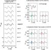 |
Fig. 7 a) Temporal evolution of Stokes V profile of pixel P iv located in patch A. b) Two-magnetic component SIR inversion of Stokes profiles at P iv at 19:58 UT. The wavelength scale is given in Δ λ from the Fe i 630.15 nm line rest wavelength position. Upper: Stokes I profile and the Stokes I profile retrieved from the inversion (red dashed line). Lower right: observed Stokes V profile (black solid line) and Stokes V profile from the best-fit inversion (red dashed line). The rest wavelengths for both Fe i 630.15 nm and Fe i 630.25 nm are indicated by vertical lines. Lower left: Stokes V profiles synthesized from the two individual magnetic atmospheres without taking their respective filling factors into account (green and blue lines). The atmospheric parameters from this inversion can be found in Table 1. c) Simple Gaussian fit to the observed Stokes V profile of a pixel close to P iv and also located in patch A. The slit scan containing this pixel was taken approximately 1 s earlier than the profile at P iv. The rest wavelengths for both Fe i 630.15 nm and Fe i 630.25 nm are indicated by vertical lines. Upper row: two anti-symmetric Stokes V profiles constructed with Gaussians and shifted with respect to each other. On the right the combination of the two synthetic anti-symmetric Stokes V profiles is shown as a red dashed line. Lower row: on the left side we show a synthetic negative polarity Stokes V profile (green line) and a reversed polarity Stoke V profile (blue). On the right side we show again the combination of the two synthetic anti-symmetric Stokes V profiles as a red dashed line. |
Possible explanations for this low polarization signal are strong magnetic fields that cancel each other within the resolution element or/and a high (possibly polarized) stray-light factor or/and local heating, which cause a change in the line profile. The continuum intensity is at 20% of the quiet-Sun intensity at these locations. Previous studies of the umbral atmosphere at very strong magnetic field locations suggest an intensity of ~10% in our wavelength range (Maltby 1970). On close inspection, one finds that the splitting is more discernible in the Stokes I profile of the Fe i 630.25 nm line at P i than in P iv or P iii, and one can distinguish between three distinct components in the Stokes I profile. These two observations hint at a high stray-light factor in this region.
The low polarization signature remains the same for the entire observing time in patch B. In patch A, however, the polarization signal becomes even more reduced and we observe multilobed profiles in one of the Fe i lines during flaring activity. The temporal evolution of the Stokes V profiles located at P iv (patch A) is shown in Fig. 7a. Between 19:47 and 20:07 UT, during the rising phase in the SXR flux of flare iii, one can observe asymmetric multilobed profiles only in the Fe i 630.15 nm line at PIV. Only the Fe i 630.15 nm line is affected because of the line formation region difference between the two lines that is estimated (for non-magnetized regions) at 64 km (Faurobert et al. 2009) with the Fe i 630.15 nm being formed in higher layers in the atmosphere. This means that the atmospheric parameters responsible for the observed asymmetry change their properties over a very short height range along the line of sight in the line formation region. If the low polarization signal and the short-lived multilobe profiles were caused by a real opposite polarity emerging, we would expect the line with a formation region lower in the atmosphere (Fe i 630.25 nm) to be more affected. Because this is not the case, we exclude this possibility.
We performed SIR inversions on the multilobed profiles taking only the spectral window of the Fe i 630.15 nm line into account. We allowed for two magnetized atmospheres within the resolution element and an unpolarized stray-light component. The best-fit synthesized profile for the Stokes V and I profile at location P iv are shown in Fig. 7b. The corresponding retrieved atmospheric parameters are listed in Table 1, where v is the line-of-sight velocity, B the magnetic field, T the temperature, γ the inclination angle, and f the filling factor. The Stokes V profile in green is the profile synthesized from the umbra model 1 and the Stokes V profile in blue emerges from umbra model 2. Negative line-of-sight velocity values correspond to an upflow. The Stokes Q and Stokes U signals were below the noise. The inversion results in a stray-light factor of 14.2% and the two magnetized atmospheres exhibit a line-of-sight velocity difference of ~12 km s-1 with an upflow of 4.64 km s-1 and a downflow of 7.35 km s-1.
We were unable to invert some of the pixels in patch A and we used a simple fitting approach for these cases employing constructed Gaussians as described in Sect. 2.3.
Atmospheric parameters for the two magnetic atmospheres obtained by a SIR inversion.
In Fig. 7c we show such a fit for a pixel that is also located in patch A and close to P iv. Depending on the start model (same polarity or opposite polarity atmospheres) we arrived at different fit solutions and obtained two possible atmospheric scenarios that could cause the asymmetric Stokes V profile. The profile can be reproduced by two same-polarity synthetic Stokes V profiles with a high velocity difference. The best fit achieved in this way produces a line-of-sight velocity difference of ~13.3 km s-1. Calibrating the wavelength scale with the telluric line position, the blue-shifted line has a velocity of ~8.2 km s-1 and the red-shifted line exhibits a velocity of ~5.1 km s-1. The second possibility is that a locally heated atmosphere causes the complex emerging Stokes V profile, as has been found previously by e.g. Socas-Navarro et al. (2000b) in their umbral flash studies using the Ca ii infrared triplet. They observed short-lived asymmetric Stokes V profiles in the sunspot umbra and were able to show that these are caused by the combination of two unresolved atmospheric components, one resulting in a normal Stokes V profile and the second producing a blueshifted reversed Stokes V signal through an emission process. In the second row in Fig. 7c we demonstrate this possibility with our simple Gaussian model. We fit the profile using a Stokes V signal as it would arise if caused by absorption and a reversed polarity signal caused by an emission feature. The reversed Stokes V profile exhibits a narrower profile that could arise because the emission feature is mainly present in the core of the spectral line. The line-of-sight velocity difference between the two anti-symmetric profiles is ~0.48 km s-1.
Because the multilobed profiles appear in a strong magnetic field location with a high stray-light percentage in which the polarization signal is already reduced in amplitude, the effect of the spectral line going into emission is visible in Stokes V while the line core reversal can be completely masked in Stokes I, as was demonstrated in Vitas (2011). He synthesized profiles from MURaM snapshots (Vögler & Schüssler 2003, see code description) and showed that the expected line reversal in the Stokes I profile emerging from an atmosphere with a temperature increase with height was masked by adding a small stray-light contamination, while the Stokes V profiles maintained a complex shape.
For a large velocity difference as well as for the local heating scenario, a good fit is achieved using two anti-symmetric Stokes V profiles. This indicates a multicomponent magnetic atmosphere and subresolution fine structure.
3.3. Sign reversal in MDI magnetograms and RHESSI reconstruction
We selected MDI magnetograms before, during, and after the GOES SXR flux peaks of flares i, iii, and v. The magnetograms are shown in Fig. 8 and are labeled a to i. The times corresponding to these letters can be found in Fig. 9. During the soft X-ray flux rising times of flare i (panel b in Fig. 8) one can observe a patch (co-spatial with patch A from Fig. 4) that exhibits an apparent reversed polarity in the negative umbra before it is reduced in amplitude shortly afterward (panel c). During flare iii the reversed polarity, located at patch A, is more prominent during the SXR flux rising phase (panel e). The last flare shows an elongated structure that exhibits a strong sign reversal and spans over the PIL connecting patches A and B.
The MDI uses the difference of dopplergrams observed in the Stokes I − V and I + V profiles of the Ni i 676.77 nm line to quantify the magnetic field instead of Stokes V amplitude maxima, as measured by a classical magnetograph (Scherrer et al. 1995). The MDI-saturation, showing up as gray patches in the magnetogram, is caused by the low intensities measured in the strong umbra, which render the onboard processing algorithm ineffective, as shown by Liu et al. (2007). A polarity reversal, observed as a parasitic opposite polarity in an otherwise unipolar field, hints at a real physical meaning, however. If actual flux emergence is excluded, other possibilities are supersonic speeds, which would push the spectral line partly out of the analysis window, or line reversal caused by the line going into emission (Qiu & Gary 2003).
To investigate the timing relationship between the reversed polarity, multilobed Stokes V profiles observed with SOLIS, and the flare excitation, we plot the total intensity in the pixels that exhibit the reversed polarity and the number of multilobed Stokes V profiles as a function of time, and compare with the GOES SXR flux and its time derivative. The latter can usually be taken as a good proxy for the HXR time profile (via the “Neupert effect”, see e.g., Dennis & Zarro 1993), which was not continuously available throughout the event. As shown in Fig. 9, the timing of this reversed polarity and the unusual Stokes V profiles coincides very well with the derivative of the soft X-ray flux. The appearance of the apparently reversed polarity and the multilobed Stokes V profiles is therefore very likely caused by impulsive-phase, nonthermal processes that must, therefore, be affecting the photospheric layers.
This is supported by the RHESSI reconstructed images shown in Fig. 10. The data were taken during the rising SXR flux phase (see Sect. 2 for processing details). In our reconstructions (in accordance with the findings of Liu et al. 2009) we can identify a low-energy X-ray source over the negative polarity umbra that stretches on one side over the PIL into the positive umbra and at least two nonthermal HXR sources placed at the locations of patches A and B. In a classic flare picture the SXR is a loop top source of flare iii with the hard X-ray sources located at the chromospheric footpoints of the interacting loops. These footpoints are areas with high-energy electrons impacting the lower atmosphere.
 |
Fig. 8 MDI magnetograms during flares i, iii, and v. The images are all clipped to the same maximum and minimum of ± 500 G. The observation times are indicated by the vertical lines in Fig. 9 corresponding to the letters a) to i). Upper row [a), b), c)]: the first panel shows the sunspot before flare i. Panel two was taken during the rising phase of flare i and panel c after the flare SXR peak. Middle row [d), e), f)]: magnetograms before flare iii, during the rising phase of the flare and after. Lower row: [g), h), i)]: magnetograms showing the sunspot this time before flare v, during the rising phase of the flare and again after. |
 |
Fig. 9 Soft X-ray flux recorded by GOES between 19:00 UT and 23:40 UT (solid line). The dashed green line corresponds to its derivative. The dashed red line corresponds to the sum of parasitic positive magnetogram values found in patch A in the negative polarity umbra of the MDI magnetograms. The function was multiplied by a factor for the purpose of shifting the values into the plotting range. The blue dashed-dotted line is the number of multilobed Stokes V profiles observed with SOLIS and found in patch A again scaled to the plotting window. The vertical lines at the top of the figure signify the recording time of the magnetograms (a–i) displayed in Fig. 8. |
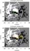 |
Fig. 10 RHESSI reconstructions during flare iii. The times refer to the MDI magnetogram. For the RHESSI reconstruction times refer to Sect. 2.4. Upper row: RHESSI low-energy X-ray reconstruction (12–18 keV) contoured at a level of 40% and overlaid onto a MDI magnetogram with the same cutoff level of ± 500 G as in Fig. 8. The low-energy X-ray emitting region is located above the PIL at the δ-spot. The blue box is the FOV chosen for the RHESSI reconstruction. Lower row: RHESSI hard X-ray reconstruction (25–50 keV) contoured at a level of 40% and overlaid onto a MDI magnetogram. The blue box is again the FOV chosen for the RHESSI reconstruction. The regions denoted A and B are the same as in Fig. 4. |
4. Discussion and conclusion
We applied a height-dependent inversion to the full Stokes profiles data of flare iii and found a change of magnetic field vector direction along the polarity inversion line. We identified regions R1 and R3, which show an increase in transversal magnetic field accompanied by a decrease in longitudinal magnetic field and a region R2 in between that shows the opposite movement (see Fig. 5). These regions are located close to the PIL that separates the umbrae. With their extensive multiwavelength analysis, Liu et al. (2009) have speculated on the flaring loop configuration (see their Fig. 7 panel d) of flare iii. Two of the flare kernels (their k1 and k2, corresponding to our patch A and B) are in the positive and in the negative polarity umbra, respectively, and are connected to kernels outside the δ-spot. According to Liu and collaborator’s speculation, the flare is a consequence of reconnection taking place between these loop systems just above the PIL that separates the two umbrae. After the flare, k1 and k2 are connected by a low-lying loop. This scenario agrees well with our observations because the transverse magnetic field increases on the opposite sides of the PIL (regions R1 and R3 in Fig. 5), indicating the development of a lower lying loop. The increase in longitudinal magnetic field at location R2 could be attributed to the removal of opposing longitudinal fields close to the X-point above the PIL. This is a favorable two-loop configuration in the flare model of Melrose (1997), where a longer loop and a low-lying shorter loop are formed as a consequence of reconnection between two same-polarity, co-linear, current-carrying loops crossing each other above the photosphere. Permanent changes of the magnetic field have been quantified in many flares. Sudol & Harvey (2005) used GONG magnetograms to identify magnetic field changes and found that the changes were often abrupt (less than 10 min) and permanent. More recent observations from Wang et al. (2012) taken with the SDO/HMI instrument also show an enhancement in horizontal field by 30% taking place within ~30 min in an area close to the PIL during an X 2.2 flare. Our findings show that the changes occur during almost the entire time sequence (90 min) and are therefore not sudden. In addition, flare iii occurs after two previous flares, and we do not have enough coverage before and after the flares to compare the field changes in the same area when not affected by a flare.
We found two locations of strong magnetic field A and B, as inferred from the corresponding Stokes I profiles, that show a low polarization signal (less than 30% than in their surrounding). Profiles located in patch A, such as P iv, also show multilobed asymmetric Stokes V profiles during flare activity co-spatial and co-temporal with a reversed polarity signal in MDI magnetograms and a hard X-ray source observed with RHESSI. The asymmetry seen in Stokes V lasts for about 15 to 20 min and occurs during the impulsive phase of flare iii and only in the Fe i 630.15 nm line. Because the Fe i 630.25 nm line is not affected and is formed about 64 km deeper than the Fe i 630.15 nm line, this indicates a very rapid variation of the atmospheric properties with depth.
The temporarily reversed magnetic polarity patch, if indeed caused by an actual magnetic feature and not by the disturbance of the spectral lines caused by flare heating, is reminiscent of the magnetic configuration described by Falconer et al. (2000). In this, an isolated patch of one “included” polarity surrounded by the opposite polarity gives rise to a coronal null and a “spine-fan” magnetic topology – which is also central to flares studied by Aulanier et al. (2000) and Fletcher et al. (2001). However, unlike in these models, the reversed polarity patch in our flare is not stable and does not persist after the flare, but is a transient feature. Moreover, because the multilobe profile is observed only in the Fe i 630.15 nm line, it is also reasonable to exclude flux emerging at these times.
From our fits we find at least two possible atmospheric scenarios that are capable of reproducing these profiles. One is a two-component atmosphere exhibiting a velocity difference between the components in the range of 12 km s-1 to 14 km s-1, or alternatively a polarity-reversed contribution to the emerging Stokes V profile due to a temperature increase from the local back-warming from the chromosphere. Because this effect can be masked in Stokes I by a small filling factor of the reversed signal and a high stray-light factor at this location, we were unable to distinguish between these two cases.
Observation of high velocities deduced from asymmetric Stokes V profiles in a sunspot were also found by Martinez Pillet et al. (1994) and Meunier & Kosovichev (2003). In both cases they were observed close to the PIL in a δ-sunspot. The Martinez Pillet et al. (1994) Stokes V fit showed velocities of 14 km s-1, but these were long-lasting flows and in the observations of Martinez Pillet et al. (1994) seemingly unconnected to a flare. A transient flow of 2 km s-1 at flare footpoints was reported recently by Martínez Oliveros et al. (2011) deduced from line shifts in the intensity profiles observed with the HMI onboard SDO during a whitelight flare. A downflow of 8 km s-1 was found in the Na D1 line (lower chromosphere) by Donea & Lindsey (2005), in association with the launch of a flare seismic wave, and transient downflows have also been reported earlier by Kosovichev (2006). Indeed, a popular model for launching the flare seismic waves is strong local heating in the chromosphere that leads to downward-propagating hydrodynamic shocks, as found by Fisher et al. (1985), which deliver energy and momentum to the photosphere.
Apparent flux reversals in magnetograms during flares have been reported previously by, e.g., Patterson (1984) and Qiu & Gary (2003). Qiu & Gary (2003) also found co-spatial HXR sources at the reversed polarity sites. These authors simulated the MDI signal in Ni i 676.77 nm and suggested that the signal is caused by the line center or even the whole line going into emission. They found an interesting connection between locations of a strong magnetic field and reversed polarity sites and pointed out that this could be because only at these locations the energy requirement to produce the effect is low enough. Our case supports this because we found the asymmetric Stokes profiles only at the site of lowest continuum intensity in the umbra (see Fig. 4, green contours on the TRACE whitelight image), which therefore favors the local heating scenario. Maurya et al. (2012) have observed an apparently reversed polarity in HMI magnetograms during a 2.2 X-flare. These authors obtained the spectral line profile (six spectral points) and found an intensity enhancement near the line core that was correlated temporally to the impulsive phase of the flare. Similar observational signatures were accordingly seen in several spectral lines from Ni i 676.77 nm (MDI) to Fe i 617.33 nm (HMI) and Fe i 630.15 nm (SOLIS-VSM).
Our analysis confirms the direct connection between the chromospheric flare response and the photospheric atmosphere as seen in the Stokes profiles. Although we cannot distinguish between the two physical explanations, it is clear that the flare impact sites show a fine structure in the photosphere. Although a fine structure in the umbra, as we observed, seems surprising, this has already been suggested by e.g., Socas-Navarro et al. (2000a) who studied asymmetric Stokes V profiles in the infrared Ca II lines. These authors observed very similar short-lived unusual Stokes V profiles and were only able to invert the profiles with a sub-arcsec multicomponent atmosphere in the sunspot umbra. With the sub-arcsec resolution of instruments such as Hinode it has been possible to actually observe this fine structure directly in the chromosphere (Socas-Navarro et al. 2009).
Full Stokes profile observations during a flare with high spatial, spectral, and temporal resolution that probe, in addition to the photosphere also the higher atmospheric layers through multi-wavelength observations are needed to be able to distinguish between the possible atmospheric scenarios that lead to the anomalies seen in longitudinal magnetograms and as asymmetric Stokes V profiles. However, owing to the current spatial resolution and the unpredictability of flare onset, the study of flare triggering mechanism, flare impact, and photospheric response is still challenging. We have shown that fine structure is also important in areas of strong magnetic fields as encountered in sunspot umbrae and that the high-resolution study of flare footpoints offers the possibility of understanding the coupling between the atmospheric layers in flare processes.
Acknowledgments
We thank Aimee Norton for her correspondence concerning MDI saturation features. This research project has been supported by a Marie Curie Early Stage Research Training Fellowship of the European Community’s Sixth Framework Program under contract number MEST-CT-2005-020395. L. Fletcher acknowledges support from STFC Grant ST/1001808 and the EC-funded FP7 project HESPE (FP7-2010-SPACE-1-263086). The project has been also supported by the SOLAIRE network of the European Community’s Sixth Framework Programme.
References
- Aboudarham, J., & Henoux, J. C. 1986, A&A, 156, 73 [NASA ADS] [Google Scholar]
- Archontis, V., & Hood, A. W. 2010, A&A, 514, A56 [NASA ADS] [CrossRef] [EDP Sciences] [Google Scholar]
- Aulanier, G., DeLuca, E. E., Antiochos, S. K., McMullen, R. A., & Golub, L. 2000, ApJ, 540, 1126 [NASA ADS] [CrossRef] [Google Scholar]
- Bellot Rubio, L. 2003, Inversion of Stokes profiles with SIR (Freiburg: Kiepenheuer Inst. Sonnenphysik) [Google Scholar]
- Cameron, R., & Sammis, I. 1999, ApJ, 525, L61 [NASA ADS] [CrossRef] [Google Scholar]
- Canou, A., Amari, T., Bommier, V., et al. 2009, ApJ, 693, L27 [NASA ADS] [CrossRef] [Google Scholar]
- Carmichael, H. 1964, NASA Sp. Publ., 50, 451 [Google Scholar]
- Chifor, C., Tripathi, D., Mason, H. E., & Dennis, B. R. 2007, A&A, 472, 967 [Google Scholar]
- Dennis, B. R., & Zarro, D. M. 1993, Sol. Phys., 146, 177 [NASA ADS] [CrossRef] [Google Scholar]
- Donea, A.-C., & Lindsey, C. 2005, ApJ, 630, 1168 [NASA ADS] [CrossRef] [Google Scholar]
- Engell, A. J., Siarkowski, M., Gryciuk, M., et al. 2011, ApJ, 726, 12 [NASA ADS] [CrossRef] [Google Scholar]
- Falconer, D. A., Gary, G. A., Moore, R. L., & Porter, J. G. 2000, ApJ, 528, 1004 [NASA ADS] [CrossRef] [Google Scholar]
- Faurobert, M., Aime, C., Périni, C., et al. 2009, A&A, 507, L29 [NASA ADS] [CrossRef] [EDP Sciences] [Google Scholar]
- Fischer, C. E., Keller, C. U., & Snik, F. 2009, in ASP Conf. Ser., 405, eds. S. V. Berdyugina, K. N. Nagendra, & R. Ramelli, 311 [Google Scholar]
- Fisher, G. H., Canfield, R. C., & McClymont, A. N. 1985, ApJ, 289, 434 [NASA ADS] [CrossRef] [Google Scholar]
- Fletcher, L., & Hudson, H. S. 2008, ApJ, 675, 1645 [NASA ADS] [CrossRef] [Google Scholar]
- Fletcher, L., Metcalf, T. R., Alexander, D., Brown, D. S., & Ryder, L. A. 2001, ApJ, 554, 451 [NASA ADS] [CrossRef] [Google Scholar]
- Fletcher, L., Hannah, I. G., Hudson, H. S., & Metcalf, T. R. 2007, ApJ, 656, 1187 [NASA ADS] [CrossRef] [Google Scholar]
- Frutiger, C., & Solanki, S. K. 1998, A&A, 336, L65 [NASA ADS] [Google Scholar]
- Georgoulis, M. K. 2005, ApJ, 629, L69 [NASA ADS] [CrossRef] [Google Scholar]
- Handy, B. N., Acton, L. W., Kankelborg, C. C., et al. 1999, Sol. Phys., 187, 229 [NASA ADS] [CrossRef] [Google Scholar]
- Hirzberger, J., Riethmüller, T., Lagg, A., Solanki, S. K., & Kobel, P. 2009, A&A, 505, 771 [NASA ADS] [CrossRef] [EDP Sciences] [Google Scholar]
- Hurford, G. J., Schmahl, E. J., Schwartz, R. A., et al. 2002, Sol. Phys., 210, 61 [NASA ADS] [CrossRef] [Google Scholar]
- Keller, C. U., & SOLIS Team 2003, BAAS, 35, 848 [NASA ADS] [Google Scholar]
- Kleint, L. 2012, ApJ, 748, 138 [NASA ADS] [CrossRef] [Google Scholar]
- Kopp, R. A., & Pneuman, G. W. 1976, Sol. Phys., 50, 85 [NASA ADS] [CrossRef] [Google Scholar]
- Kosovichev, A. G. 2006, Sol. Phys., 238, 1 [NASA ADS] [CrossRef] [Google Scholar]
- Kosovichev, A. G. 2007, ApJ, 670, L65 [NASA ADS] [CrossRef] [Google Scholar]
- Kosovichev, A. G., & Zharkova, V. V. 1998, Nature, 393, 317 [NASA ADS] [CrossRef] [Google Scholar]
- Kubo, M., Yokoyama, T., Katsukawa, Y., et al. 2007, PASJ, 59, 779 [NASA ADS] [Google Scholar]
- Kusano, K., Maeshiro, T., Yokoyama, T., & Sakurai, T. 2002, ApJ, 577, 501 [NASA ADS] [CrossRef] [Google Scholar]
- Lin, R. P., Dennis, B. R., Hurford, G. J., et al. 2002, Sol. Phys., 210, 3 [Google Scholar]
- Liu, Y., Norton, A. A., & Scherrer, P. H. 2007, Sol. Phys., 241, 185 [NASA ADS] [CrossRef] [Google Scholar]
- Liu, C., Lee, J., Karlický, M., et al. 2009, ApJ, 703, 757 [NASA ADS] [CrossRef] [Google Scholar]
- Machado, M. E., & Rust, D. M. 1974, Sol. Phys., 38, 499 [NASA ADS] [CrossRef] [Google Scholar]
- Machado, M. E., Emslie, A. G., & Avrett, E. H. 1989, Sol. Phys., 124, 303 [NASA ADS] [CrossRef] [Google Scholar]
- Maltby, P. 1970, Sol. Phys., 13, 312 [NASA ADS] [CrossRef] [Google Scholar]
- Martínez Oliveros, J. C., Couvidat, S., Schou, J., et al. 2011, Sol. Phys., 269, 269 [NASA ADS] [CrossRef] [Google Scholar]
- Martinez Pillet, V., Lites, B. W., Skumanich, A., & Degenhardt, D. 1994, ApJ, 425, L113 [NASA ADS] [CrossRef] [Google Scholar]
- Maurya, R. A., Vemareddy, P., & Ambastha, A. 2012, ApJ, 747, 134 [NASA ADS] [CrossRef] [Google Scholar]
- Melrose, D. B. 1997, ApJ, 486, 521 [NASA ADS] [CrossRef] [Google Scholar]
- Metcalf, T. R., Canfield, R. C., & Saba, J. L. R. 1990, ApJ, 365, 391 [NASA ADS] [CrossRef] [Google Scholar]
- Meunier, N., & Kosovichev, A. 2003, A&A, 412, 541 [NASA ADS] [CrossRef] [EDP Sciences] [Google Scholar]
- Müller, D. A. N., Schlichenmaier, R., Fritz, G., & Beck, C. 2006, A&A, 460, 925 [NASA ADS] [CrossRef] [EDP Sciences] [Google Scholar]
- Nagashima, K., Isobe, H., Yokoyama, T., et al. 2007, ApJ, 668, 533 [NASA ADS] [CrossRef] [Google Scholar]
- Patterson, A. 1984, ApJ, 280, 884 [NASA ADS] [CrossRef] [Google Scholar]
- Qiu, J., & Gary, D. E. 2003, ApJ, 599, 615 [NASA ADS] [CrossRef] [Google Scholar]
- Ruiz Cobo, B., & del Toro Iniesta, J. C. 1992, ApJ, 398, 375 [NASA ADS] [CrossRef] [Google Scholar]
- Scherrer, P. H., Bogart, R. S., Bush, R. I., et al. 1995, Sol. Phys., 162, 129 [Google Scholar]
- Shibata, K., & Magara, T. 2011, Liv. Rev. Sol. Phys., 8, 6 [Google Scholar]
- Sigwarth, M. 2001, ApJ, 563, 1031 [NASA ADS] [CrossRef] [Google Scholar]
- Skumanich, A., & Lites, B. W. 1987, ApJ, 322, 473 [Google Scholar]
- Skumanich, A., & Lites, B. 1991, in Solar Polarimetry, ed. L. J. November, 307 [Google Scholar]
- Socas-Navarro, H. 2001, in Advanced Solar Polarimetry – Theory, Observation, and Instrumentation, ed. M. Sigwarth, ASP Conf. Ser., 236, 487 [Google Scholar]
- Socas-Navarro, H. 2007, ApJS, 169, 439 [NASA ADS] [CrossRef] [Google Scholar]
- Socas-Navarro, H., Trujillo Bueno, J., & Ruiz Cobo, B. 2000a, ApJ, 544, 1141 [NASA ADS] [CrossRef] [Google Scholar]
- Socas-Navarro, H., Trujillo Bueno, J., & Ruiz Cobo, B. 2000b, Science, 288, 1396 [NASA ADS] [CrossRef] [Google Scholar]
- Socas-Navarro, H., McIntosh, S. W., Centeno, R., de Wijn, A. G., & Lites, B. W. 2009, ApJ, 696, 1683 [NASA ADS] [CrossRef] [Google Scholar]
- Sturrock, P. A., & Coppi, B. 1966, ApJ, 143, 3 [NASA ADS] [CrossRef] [Google Scholar]
- Sudol, J. J., & Harvey, J. W. 2005, ApJ, 635, 647 [NASA ADS] [CrossRef] [Google Scholar]
- Vitas, N. 2011, Ph.D. Thesis, Sterrekundig Instituut Utrecht [Google Scholar]
- Viticchié, B., & Sánchez Almeida, J. 2011, A&A, 530, A14 [NASA ADS] [CrossRef] [EDP Sciences] [Google Scholar]
- Vögler, A., & Schüssler, M. 2003, Astron. Nachr., 324, 399 [NASA ADS] [CrossRef] [Google Scholar]
- Wang, H., Liu, C., Jing, J., & Yurchyshyn, V. 2007, ApJ, 671, 973 [NASA ADS] [CrossRef] [Google Scholar]
- Wang, S., Liu, C., Liu, R., et al. 2012, ApJ, 745, L17 [NASA ADS] [CrossRef] [Google Scholar]
- Xu, Y., Cao, W., Liu, C., et al. 2004, ApJ, 607, L131 [Google Scholar]
All Tables
Atmospheric parameters for the two magnetic atmospheres obtained by a SIR inversion.
All Figures
|
Fig. 1 Active region NOAA 10808 on September 13, 2005. Left: magnetogram obtained from SOLIS-VSM Stokes V profile amplitudes in the Fe i 630.25 nm line. The white areas denote positive magnetic flux, while the black areas are regions exhibiting negative magnetic flux. The orange line shows the intricate polarity inversion line (PIL). Right: co-spatial intensity image constructed from the Stokes I continuum intensities. |
| In the text | |
|
Fig. 2 GOES X-ray flux recorded on September 13, 2005. The flare numbers, adapted from Liu et al. (2009), are indicated with capital roman numbers. The second flare is not discernible in the soft X-ray flux. The SOLIS-VSM observation time from 19:36 UT to 20:57 UT is represented by the red solid line. MDI, recording magnetograms in Ni i 676.77 nm, and the RHESSI observing times are indicated with green dashed-dotted and blue dashed lines, respectively. |
| In the text | |
|
Fig. 3 RHESSI light curves on September 13, 2005. The light curves were corrected for attenuator and decimation state changes. The rate is shown for various energy bands and is an average over 6 detectors. The SOLIS observation time is indicated with a dashed horizontal line. |
| In the text | |
|
Fig. 4 Umbral region of NOAA 10808, before and after flare iii. Top row: the TRACE whitelight intensity image on the left side in the upper row was recorded at 19:36 and rotated and scaled to the SOLIS-VSM data. The green contours are locations where the continuum intensity is below ~20% of the quiet Sun continuum. These regions marked as A and B are also locations of low polarization signals. The second panel in the upper row is the SOLIS magnetogram that was obtained from the Stokes V profiles (see main text for details) recorded at about 19:56 UT. The last two panels, magnetic field strength in kG and inclination angle γ, are the result of LILIA inversions of the SOLIS-VSM full Stokes profiles recorded around 19:56 UT at optical depth log (τ500 nm) = -1. The inclination angle is shown in degrees, with a magnetic field vector along the line of sight pointing out of the solar surface with an inclination angle of 0° . The black lines are contours obtained by choosing cutoff levels of 0.002 and −0.002 for the magnetogram. The black areas in the inversion results are uninverted pixels. The noise produced by the deteriorating polarization modulator propagates into the inversion results. Bottom row: the first panel shows the TRACE whitelight image at 20:10 UT. The last three panels in the lower row are the magnetogram and the inversion results obtained from SOLIS data recorded around 20:05 UT. The Stokes profiles found at locations P i to P iv are discussed in Sect. 3.2. |
| In the text | |
|
Fig. 5 Top row: TRACE whitelight image. Purple contours show areas with changes in the magnetic field azimuth larger than 5° and yellow contours are areas in which the longitudinal magnetic field switches from a positive sign to a negative sign or the other way around. All values are retrieved through the inversion and are selected at optical depth log(τ500 nm) = -1. The second and third panels show the change in Btrans and Blong. White areas are regions of increase in Btrans/Blong and areas of decrease are black. R1 (red contour), R2 (purple contour), and R3 (yellow contour) in the last panel are locations of simultaneous change in Btrans and Blong greater than 400 G in both parameters. Last three rows: average inclination angle γ and the average Btrans in the regions R1, R2, and R3. As in Fig. 4, the inclination angle runs from 0° to 180° with γ = 90 °, representing a transversal magnetic field and an angle of γ > 90 °, constituting a negative longitudinal magnetic field (vector pointing toward the Sun). The error bars are the standard deviation in γ and Btrans over a region in the umbra outside the flare site. The soft X-ray GOES curve is overlaid in blue. |
| In the text | |
|
Fig. 6 Quiet-Sun profile and Stokes profiles retrieved from the positions P i to P iv marked in Fig. 4. The columns show Stokes I with the two Fe i 630 nm lines and two telluric oxygen lines normalized to an averaged quiet-Sun Stokes I continuum to demonstrate the continuum intensity differences and Stokes Q, U and V profiles normalized to the local Stokes I continuum to show the differences in scales between the polarization signals. The wavelength scale is given in Δ λ from the Fe i 630.15 nm rest wavelength position. The full-width at half-maximum is given for the Fe i 630.15 nm line. The red curve overplotted on the profiles located at P I denotes synthesized profiles fitted to the observations by the inversion code. The magnetic and velocity field values at log (τ500 nm = -1) corresponding to this fit are B = 2.1 kG with an inclination angle of γ = 25 ° and a velocity of vLOS = −1.5 km s-1. |
| In the text | |
|
Fig. 7 a) Temporal evolution of Stokes V profile of pixel P iv located in patch A. b) Two-magnetic component SIR inversion of Stokes profiles at P iv at 19:58 UT. The wavelength scale is given in Δ λ from the Fe i 630.15 nm line rest wavelength position. Upper: Stokes I profile and the Stokes I profile retrieved from the inversion (red dashed line). Lower right: observed Stokes V profile (black solid line) and Stokes V profile from the best-fit inversion (red dashed line). The rest wavelengths for both Fe i 630.15 nm and Fe i 630.25 nm are indicated by vertical lines. Lower left: Stokes V profiles synthesized from the two individual magnetic atmospheres without taking their respective filling factors into account (green and blue lines). The atmospheric parameters from this inversion can be found in Table 1. c) Simple Gaussian fit to the observed Stokes V profile of a pixel close to P iv and also located in patch A. The slit scan containing this pixel was taken approximately 1 s earlier than the profile at P iv. The rest wavelengths for both Fe i 630.15 nm and Fe i 630.25 nm are indicated by vertical lines. Upper row: two anti-symmetric Stokes V profiles constructed with Gaussians and shifted with respect to each other. On the right the combination of the two synthetic anti-symmetric Stokes V profiles is shown as a red dashed line. Lower row: on the left side we show a synthetic negative polarity Stokes V profile (green line) and a reversed polarity Stoke V profile (blue). On the right side we show again the combination of the two synthetic anti-symmetric Stokes V profiles as a red dashed line. |
| In the text | |
|
Fig. 8 MDI magnetograms during flares i, iii, and v. The images are all clipped to the same maximum and minimum of ± 500 G. The observation times are indicated by the vertical lines in Fig. 9 corresponding to the letters a) to i). Upper row [a), b), c)]: the first panel shows the sunspot before flare i. Panel two was taken during the rising phase of flare i and panel c after the flare SXR peak. Middle row [d), e), f)]: magnetograms before flare iii, during the rising phase of the flare and after. Lower row: [g), h), i)]: magnetograms showing the sunspot this time before flare v, during the rising phase of the flare and again after. |
| In the text | |
|
Fig. 9 Soft X-ray flux recorded by GOES between 19:00 UT and 23:40 UT (solid line). The dashed green line corresponds to its derivative. The dashed red line corresponds to the sum of parasitic positive magnetogram values found in patch A in the negative polarity umbra of the MDI magnetograms. The function was multiplied by a factor for the purpose of shifting the values into the plotting range. The blue dashed-dotted line is the number of multilobed Stokes V profiles observed with SOLIS and found in patch A again scaled to the plotting window. The vertical lines at the top of the figure signify the recording time of the magnetograms (a–i) displayed in Fig. 8. |
| In the text | |
|
Fig. 10 RHESSI reconstructions during flare iii. The times refer to the MDI magnetogram. For the RHESSI reconstruction times refer to Sect. 2.4. Upper row: RHESSI low-energy X-ray reconstruction (12–18 keV) contoured at a level of 40% and overlaid onto a MDI magnetogram with the same cutoff level of ± 500 G as in Fig. 8. The low-energy X-ray emitting region is located above the PIL at the δ-spot. The blue box is the FOV chosen for the RHESSI reconstruction. Lower row: RHESSI hard X-ray reconstruction (25–50 keV) contoured at a level of 40% and overlaid onto a MDI magnetogram. The blue box is again the FOV chosen for the RHESSI reconstruction. The regions denoted A and B are the same as in Fig. 4. |
| In the text | |
Current usage metrics show cumulative count of Article Views (full-text article views including HTML views, PDF and ePub downloads, according to the available data) and Abstracts Views on Vision4Press platform.
Data correspond to usage on the plateform after 2015. The current usage metrics is available 48-96 hours after online publication and is updated daily on week days.
Initial download of the metrics may take a while.