| Issue |
A&A
Volume 547, November 2012
|
|
|---|---|---|
| Article Number | A42 | |
| Number of page(s) | 17 | |
| Section | Stellar atmospheres | |
| DOI | https://doi.org/10.1051/0004-6361/201219168 | |
| Published online | 24 October 2012 | |
Testing the opacity and equation of state of LTE and non-LTE model atmospheres with OPAL and OP data for early-type stars
Astronomical Institute of the Wroclaw University,
ul. Kopernika 11,
51-622
Wroclaw,
Poland
e-mail: This email address is being protected from spambots. You need JavaScript enabled to view it.
Received: 5 March 2012
Accepted: 7 July 2012
Abstract
Context. Complex investigations of stars are made by studying their atmospheres, evolutionary states and oscillation properties, but the opacities and equation of state are still uncertain.
Aims. Compatibility of model atmospheres with internal structure of early-type stars are investigated at photospheric and sub-photospheric regions.
Methods. The problem was studied quantitatively by means of diagrams that involve the Rosseland-mean opacities, temperatures, densities, and gradients of radiation pressure as functions of depth using stellar atmosphere and envelope models.
Results. Two new grids of radiative-equilibrium models of atmospheres were calculated assuming the local thermodynamic equilibrium (LTE). The first one is based on Kurucz’s ATLAS12 computer code implemented with the occupation probability formalism, which accounts for the destruction of loosely bound states of atoms by interactions with particles in the plasma. The second grid of models is based on monochromatic opacities and equations of state taken from the well-known international opacity project (OP). Non-LTE model atmospheres are also calculated and some aspects of the modeling are pointed out to improve agreement with ATLAS12, OP data, as well as with results of the Rogers & Iglesias OPAL opacity computing code (OPAL). The model atmospheres are also discussed by analyzing emerging fluxes of radiation.
Conclusions. Commonly used LTE and non-LTE models of stellar atmospheres of early-type stars differ markedly from each other and do not fit OPAL or OP stellar envelope models at great optical depths. The results of the OP project distributed as the OPCD v 3.3 base are useful for calculating not only stellar envelopes but also fully line-blanketed LTE model atmospheres. These models have diagnostic values for studying the atomic physics used for modeling of photospheric and sub-photospheric regions of stars.
The OPAL and OP opacities are markedly underestimated in comparison with the Rosseland-mean opacities taken from the Castelli & Kurucz (2003, IAU Symp., 210, 10) atmosphere models in which a new opacity bump appears at lgT ≈ 5.06. This additional opacity bump affects the OPAL- and OP-driving zone for stellar pulsations and therefore the new envelope models may markedly change predicted spectra of unstable oscillation modes.
Differences between current non-LTE and LTE models based on the TLUSTY200 and ATLAS codes, respectively, cannot be assigned entirely to non-LTE effects, but for B stars they reflect mainly opacity effects.
Key words: stars: early-type / radiative transfer / opacity / atomic data
© ESO, 2012
1. Introduction
Since 1970, Kurucz with coworkers published extensive grids of model atmospheres assuming the local thermodynamic equilibrium (LTE), cf. Kurucz et al. (1974), Kurucz (1979, 1999) and Castelli & Kurucz (2003), and distributed computing codes (ATLAS5, ATLAS9, ATLAS12) for the common astronomical community, cf. Kurucz (1970, 1993) and websites of Kurucz1 and Castelli2. These fully line-blanketed LTE models of atmospheres are calculated using Kurucz’s atomic data for energy levels, transition probabilities and line broadening parameters for many atoms at several ionization stages and molecules. The data are progressively updated (cf. Kurucz 2005a, 2011) and more realistic opacities and equation of state are available now from Kurucz’s website. A huge number of spectral lines (cf. Kurucz 2011) can be included in calculations by using either opacity distribution functions (ODFs) or an opacity sampling (OS) approach. The first method is commonly used to construct models of atmospheres, whereas the second one is employed to obtain synthetic spectra for a given model of atmosphere. The new version of the ATLAS12 code (Kurucz 2005a) is dedicated to calculating atmospheric models within the OS approach. In this case opacities are calculated by the line-by-line method and no synthetic spectra must by recalculated because the radiation field at the final iteration should also give the correct emerging energy distribution, which can be compared with observations.
Non-LTE models of atmospheres and computing codes were elaborated and disseminated by Mihalas and Hubeny with coworkers (Mihalas 1972; Mihalas et al. 1975; Hubeny 1988; Hubeny & Lanz 1995, 2006; Lanz & Hubeny 2003, 2007). The Hubeny code is known as TLUSTY (Hubeny 1988) and the latest distributed version has the number 200, cf. TLUSTY website3. The state-of-the-art of line-blanketed non-LTE model atmospheres were recently calculated by Lanz & Hubeny (2003, 2007) for stars with Teff ≥ 15 000 K. Although extensive model atoms of most abundant elements are used, non-LTE synthetic spectra were recalculated for a more complete list of line transitions with the best known broadening mechanisms of bound-bound transitions and were then distributed for general use through the TLUSTY website.
Since 1992, when the first results were published by Rogers & Iglesias (1992) and Iglesias & Rogers (1996) from the project based on the OPAL computing code, and by Seaton (1987), Seaton et al. (1994) and Badnell et al. (2005) from the international opacity project (OP), and by Hummer et al. (1993) from the international project of IRON devoted to compute ab-initio electron excitation cross-sections for astrophysical applications, new opportunities arise for modeling internal structure, evolution and pulsations of stars, as well as for the modeling of stellar atmospheres. Indeed, several cross-sections from the OP and IRON projects were implemented in the TLUSTY code, whereas Kurucz’s atomic data for Fe are included in OPAL and OP data. According to Seaton & Badnell (2004), the two sets of the Rosseland-mean opacities, OPAL and OP, agree between each other up to a few per cent at least up to lgT ≈ 6 despite differences in calculations of their atomic data and equation of states (EOS). In particular, the OPAL approach to the EOS is based on the many-body quantum statistical mechanics of partially ionized plasmas (cf. Rogers et al. 1996), whereas OP EOS involves the occupation probability formalism, which accounts for the destruction of loosely bound states of atoms by interactions with particles in the plasma (cf. Hummer & Mihalas 1988). The occupation probability formalism has already been used by Bergeron et al. (1991) and Tremblay & Bergeron (2009) to study hydrogen lines in atmospheres of white dwarf stars and has been implemented in the TLUSTY code by Hubeny & Lanz (1995), cf. also Hubeny et al. (1994).
In this paper we search for compatibility of LTE and non-LTE atmosphere models with stellar envelope models of early-type stars. The latter ones were calculated for the Rosseland-mean opacities and EOS taken from OPAL and OP projects. We also calculated LTE models of atmospheres using OP monochromatic opacities and OP EOS. The OP versus Kurucz treatment of autoionizing transitions has already been discussed by Castelli & Kurucz (2004). In the OP/IRON project autoionizing transitions are treated as resonances in photoionization cross-sections, cf. e.g. Bautista (1997). To make the problem tractable, each term is represented by only one level with its average energy. Kurucz treats autoionization as a line opacity with smooth continuum opacity, cf. Castelli & Kurucz (2004). In Kurucz’s approach, levels appropriate for autoionizing transitions with different quantum numbers J are included individually4.
Chemical abundances of elements.
The plan of the paper is as follows. In Sect. 2, we briefly compare published models of atmospheres with the internal structure of stars for the same effective temperature, Teff and surface gravity, lgg. Significant differences are found in optically thin and optically thick layers. We therefore calculated LTE models of atmospheres with the OS approach using the ATLAS12 computer code implemented with the occupation probability formalism (Sect. 3.1), bound-free opacities of metals from the OP/IRON project (Sect. 3.2) and detailed profiles of line absorption coefficients of H I, He I and He II (Sect. 3.3). The new ATLAS/OP code is also developed for OP monochromatic opacities and OP EOS (Sect. 3.4). Examples of the new LTE models of atmospheres of B- and O-type stars are shown in Sect. 4.1 compared with OPAL and OP models of stellar envelopes. In Sect. 4.2, ATLAS/OP models are discussed for B stars. Remarks about LTE and non-LTE models of atmospheres calculated with the TLUSTY200 computer code are made in Sect. 4.3. Synthetic spectra of the analyzed models are also plotted in Sect. 4. Finally, conclusions are given in Sect. 5.
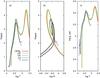 |
Fig. 1 Panel a) The Rosseland-mean opacities, κR [cm2 g-1] , as a function of lgT for Castelli & Kurucz (2003) (marked as CK line) and Lanz & Hubeny (2007) (LH line) models of |

2. Comparison of published models of atmospheres with models of envelopes
In this section the published line-blanketed LTE models of atmospheres calculated by Castelli & Kurucz (2003) and non-LTE models of Lanz & Hubeny (2003, 2007) will be briefly reviewed and compared with models of stellar envelopes calculated for the same effective temperatures and surface gravities. The atmosphere models were taken from the Castelli and TLUSTY websites. The envelope models were calculated with computer codes (ENV/OPAL and ENV/OP) developed according to the Paczynski (1969) approach, but updated to OPAL and OP opacities and EOS. OPAL data were taken from the OPAL website5 and the OP data from the CDOP v. 3.3 base (Seaton 2005) described in Sect. 3.4. All OPAL models shown in this paper have the same normalized abundances of metals, but mass fractions of hydrogen and helium are specified by X and Y numbers, respectively, cf. Table 1, where details are given together with the “standard” chemical compositions ([m/H] = 0) of the models of CK (Castelli & Kurucz 2003) and LH (Lanz & Hubeny 2007). Note that abundances of He, C, N, O, S, and Ar relative to H taken as the standard one by different authors are not the same. The abundance parameters of X, Y and Z are also shown in Table 1. As mentioned above, these numbers can be specified for OPAL data, while the chemical mixture for OP data can be fixed by users for all 17 most abundant elements (H, He, C, N, O, Ne, Na, Mg, Al, Si, S, Ar, Ca, Cr, Mn, Fe, and Ni) and therefore are not shown in Table 1. The reference chemical composition assumed in this paper is shown in the last column of Table 1.
As an example, Fig. 1 shows CK and LH models of atmospheres of Teff = 25 000 K and lgg = 4.0 in comparison with stellar envelope models calculated for OPAL and OP data with X = 0.7347 and Z = 0.0170. Panels a–c on this figure show the diagrams κR vs. lgT, κR vs. lgR and lggrad vs. lgT, respectively. The well-known Rosseland-mean opacity, κR, is defined as 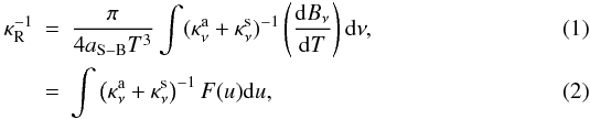 where
where ![Mathematical equation: \begin{equation} F(u) = \frac{15}{4 \pi^4} \frac{u^4 \exp(-u)}{{[1 - \exp(-u)]}^2}, \end{equation}](/articles/aa/full_html/2012/11/aa19168-12/aa19168-12-eq26.png) (3)and
(3)and  (4)Here,
  and
and  are monochromatic absorption and scattering coefficients, respectively. Bν(T) denotes the Planck function at temperature T and frequency ν and aS−B is the Stefan-Boltzmann constant. The quantity R is defined by the local values of density ρ and T:
  (5)As usual, the diffusion approximation is assumed to calculate the gradient of radiation pressure, grad, in stellar envelope codes
 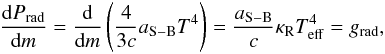 (6)whereas
  (7)for modeling of stellar atmospheres, cf. Mihalas (1978). Here, m means the mass depth, Hν the monochromatic Eddington flux of radiation, κH the flux-mean opacity and Teff the effective temperature of a star.
There are two main sources of discrepancy between the analyzed models, viz. the temperature distribution at optically thin regions and opacity effects at great optical depths. We first consider the temperature as a function of depth. The grey model of atmosphere with the optical scale corresponding to the Rosseland-mean opacities (diffusion approximation) is assumed for stellar envelope calculations. In the plane-parallel limit we have 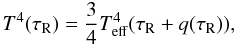 (8)where Hopf function q(τR) is in the range from 0.577 at the surface to 0.710 at great optical depths, cf. Mihalas (1978). This temperature distribution should be compared with the exact relation for the plane-parallel LTE models in radiative equilibrium, which can be expressed as
 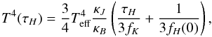 (9)where τH is the optical depth corresponding to the flux-mean opacity, κJ/κB is the ratio of the J- to B-mean opacities; fK = K/J is the Eddington factor for J (zeroth moment, mean intensity integrated over frequency) and K (second moment, so called K-integral), and fH(0) = H(0)/J(0). The CK models were calculated up to τR = 100, where T(τR = 100) ≈ 3Teff for all models of early-type stars. At great optical depths Eqs. (8) and (9) lead to the same results due to the following relations κH ≈ κR, τH ≈ τR, J ≈ B,
  and one can assume
  (Eddington approximation). The same is true for the gradients of radiation pressure, cf. Eqs. (6) and (7). One can therefore expect that atmospheric and stellar envelope models of early-type stars should agree very well with each other at the bottom of the photosphere if the Rosseland-mean opacities and densities are the same. Figure 1 shows that this is not the case. Note, however, the good agreement between OPAL and OP envelope models.
At optically thin regions the diffusion approximation (Eq. (8)) breaks down and temperature distributions of our stellar envelope models are not correct. Equation (9) indicates that the true temperature distribution of LTE models in radiative equilibrium depends on the radiation field in a much more complicated manner than the diffusion approximation predicts. Again, the same is true for the gradient of radiation pressure. Furthermore, at optically thin regions non-LTE effects may also play an important role. However, the LH model (cf. Fig. 1) does not agree either with the envelope nor CK models at optically thick regions, where LTE conditions and diffusion approximations are fulfilled with high accuracy. Clearly, the non-LTE models of Lanz & Hubeny (2003, 2007) underestimate stellar opacities.
As mentioned above, Fig. 1b shows κR versus lgR defined by Eq. (5). The stellar envelope models are plotted up to lgT = 5.68, while the CK and LH models ended at lgT = 4.87 and 5.0, respectively. The two local maxima of stellar opacities at lgT = 4.6 and lgT = 5.3 (cf. Fig. 1a) result in two loops seen on the diagram plotted in Fig. 1b. The quantity of lgR can also be expressed as lgR = lgPg − 4lgT + lgμ + 33.86, where Pg is the gas pressure and μ – mean atomic mass. The gradient of the total pressure,  , follows from the hydrostatic equilibrium equation. At optically thick regions the gradient of radiation pressure mimics the behavior of κR (cf. Eq. (6)) and therefore affects gas pressure, density, and stellar opacity in layers where κR has local maxima. This is the reason why two loops are seen in Fig. 1b.
The gradient of the radiation pressure plotted in Fig. 1c can also be compared with the gravity acceleration of lgg = 4.0, which means that the models shown in this figure are well inside the hydrostatic equilibrium. The role of the gradient of the radiation pressure increases for stars with lower lgg and higher Teff values.
We also calculated OPAL and OP Rosseland-mean opacities for the input parameters of lgT and lgρ taken from CK models. This approach has the advantage that differences in gradients of radiation pressure, geometry of models, etc. do not influence the results. Discrepancies between the CK and OPAL, and OP data approach a factor of about 2 at lgT ≈ 5.06 for the model of Teff = 45 000 K and lgg = 5.
More details about OPAL and OP data are shown in Fig. 2a−c, where the Rosseland-mean opacities, the ratio of OP to OPAL Rosseland-mean opacities and the ratio of gas pressures as functions of lgT are plotted. OP data were calculated for the input parameters (lgT and lgρ) taken from ENV/OPAL model of envelope shown in Fig. 2a. The abundance parameters equal to X = 0.7080 and Z = 0.0172 and OPAL mixture of metals listed in Table 1 were used in both cases. Evidently, OPAL and OP opacities differ from each other by a few percent at atmospheric layers, but differences can reach about 20 per cent at lgT ≈ 5.5. Although the OPAL and OP equations of state are based on different approaches, the resulting gas pressures are almost the same, cf. Fig. 2c. The agreement is better than 0.1 per cent for the chemical composition used here.
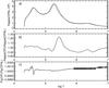 |
Fig. 2 Panel a) The Rosseland-mean opacities, κR [cm2 g-1] , as a function of lgT for OPAL (thick line) and OP (thin line) models of Teff = 25 000 K and lgg = 4.0. The chemical abundance parameters X = 0.708 and Z = 0.0172 are assumed. Panel b) The ratio of OP to OPAL Rosseland-mean opacities are displayed for input parameters of (lgT and lgρ) taken from the OPAL model shown in panel a). Panel c) The same as panel b), but for gas pressures. |
3. Modifications of the ATLAS12 code
3.1. ATLAS12/MHD-Q code
Most of the basic physical assumptions remain the same as those used in the ATLAS12 computing code distributed by Kurucz (cf. Sect. 1). Only significant changes from this code will be described here. Assuming LTE, we need to know the atomic internal partition functions for a given element k at different ionization states j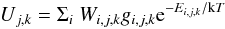 (10)to calculate occupations of atomic levels (Boltzman equations)
  (11)and ionization stages (Saha equations)
  (12)of species, cf. Mihalas (1978). Formally, the partition functions diverges if the sum extends over an infinite number of bound states of an isolated atom. In reality, the highest levels cannot remain bound because they are strongly perturbed by neighboring particles. Several theories were developed, cf. Hummer & Mihalas (1988). In particular, Kurucz (1970) assumed that levels with very high quantum number have a definite cutoff (Wi,j,k = 0) and that bound levels (Wi,j,k = 1) maintain their original values. This effect was described in terms of lowering of the ionization energy by the amount of
  (13)where ΔE is in eV, Za is 1 for neutral particles, 2 for those of once ionized, etc., and D is the Debye length,
 ![Mathematical equation: \begin{equation} D = \left(\frac{{{k}} \rm T}{4 \pi e^2}\right) ^ {1/2} [ N_{\rm e} + \Sigma_{i} ~ {Z}_{i}^{2} N_{i} ] ^ {-1/2}, \end{equation}](/articles/aa/full_html/2012/11/aa19168-12/aa19168-12-eq89.png) (14)cf. also Mihalas (1978). At low temperatures the upper levels are not populated, therefore the value of the cutoff may have a small effect on the sum in Eq. (10), but at high temperatures, the cutoff determines the value of the partition function. A more detailed discussion of this point is given in Sect. 4.1.
(14)cf. also Mihalas (1978). At low temperatures the upper levels are not populated, therefore the value of the cutoff may have a small effect on the sum in Eq. (10), but at high temperatures, the cutoff determines the value of the partition function. A more detailed discussion of this point is given in Sect. 4.1.
In the ATLAS codes partition functions of all species from H (Z = 1) up to Es (Z = 99) for neutral atoms and a few first ionization stages are calculated. The data are continuously updated by Kurucz and the latest versions of the ATLAS codes include partition functions of sufficiently high ionization stages to obtain the ion populations of elements up to T ≈ 200 000 K, cf. Kurucz (2005b, 2011). In this paper models calculated with the code based on ATLAS12 with the Kurucz partition functions are denoted as ATLAS12/KPF.
As mentioned above, we implemented the occupation probability formalism (cf. Hummer & Mihalas 1988; Mihalas et al. 1988, 1990; Däppen et al. 1988; Nayfonov et al. 1999) into the ATLAS12 code. This theory is known as the MHD (Mihalas, Hummer & Däppen) formalism. Hubeny et al. (1994) extended this approach to non-LTE plasma. The partition functions are again given by Eq. (10), but now Wi,j,k means the probability that level i remains bounded despite of perturbations by neighboring particles. Levels with low values of Wi,j,k are said to be dissolved, viz. (1 − Wi,j,k) is the probability that the level i is dissolved. Hummer & Mihalas (1988) argued that Stark splitting is the most efficient mechanism leading to dissolution of levels. The occupation probability of level i is then expressed in terms of the electric microfield distribution function W(β) as  (15)The Q(β) = QH(β) functions are tabulated e.g. by Hummer (1986) for the Holtsmark theory of the distribution function of W(β) = WH(β). Here, β measures the electric microfield at the distance r from the core with a charge of Za of radiated ions in units of the mean field strength for perturber ions with a charge Zp and density Np. For the purpose of the estimations given below we note that for low β
 (16)whereas for high β
 (17)cf. Mihalas (1978). These series expansions of WH(β) lead to
  (18)and
  (19)for βi,j,k ≪ 1 (relevant to highly excited levels) and βi,j,k ≫ 1 (appropriate for low-lying levels).
When plasma correlation effects are important, the post-Holtsmark microfield distribution is used to upgrade the original formalism, cf. Hubeny et al. (1994) and Nayfonov et al. (1999). The electric microfield distribution, W(β;Zr,a), depends now on two additional parameters, the radiator charge Zr and the correlation parameter  (20)Results of numerical integrations of Eq. (15) with W(β) = W(β;Zr,a) can be approximated by
  (21)where
 ![Mathematical equation: \begin{eqnarray} f &&= \frac{0.1402 \left( x+4 {Z_{\rm r}} a^{3} \right) \beta_{i,j,k}^{3}} {1 + 0.1285 x \beta_{i,j,k}^{3/2}}, \\[-1mm] x &&= ( 1 + a )^{3.15} \end{eqnarray}](/articles/aa/full_html/2012/11/aa19168-12/aa19168-12-eq117.png) and
and  (24)The readers are kindly referred to the papers of Hubeny et al. (1994) and Nayfonov et al. (1999), where more details are given. For a Holtsmark distribution (a = Zr = 0) this formula fits the series expansions given by Eqs. (18) and (19) to 1 per cent or better for βi,j,k < 1 and βi,j,k > 3, respectively.
For normal stellar compositions of elements one can neglect the effect of perturber ions other than protons, setting Zp = 1 and Nion = Ne. Another choice discussed by Hummer & Mihalas (1988) is to distribute the positive charge equally over all ions, so that each would have a charge of  (25)Under the second circumstances the critical value of β can be estimated as
 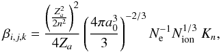 (26)where Ne = ΣZZNZ, and Nion = ΣZNZ are the total electron and ion densities, respectively, a0 is the Bohr radius, n means the principal quantum number of the state of i, and the quantal Stark-ionization correction factor is given by
 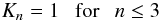 (27)and
 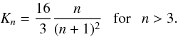 (28)We now estimate the value of the principal quantum number n′ of a level for which the occupation probability decreases to 0.9. Setting Nion = 0.9Ne into Eq. (26) and using Eq. (19) one can find βn′ = 5.3 and
 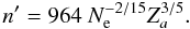 (29)For example, at the bottom of an atmosphere model of Teff = 25 000 K and lgg = 4.0, where Ne ≈ 1016 cm-3, one can obtain n′ ≈ 7 for Za = 1, whereas n′ = 61 at optically thin regions, where Ne ≈ 109 cm-3, respectively. On the other hand, one can expect that the largest atomic orbit cannot extend beyond the nearest ion, which leads to
 ![Mathematical equation: \hbox{$\langle r\rangle_{\rm nl} \approx \frac{a_0}{2 {Z}_a }[ 3 n^{2} - l ( l + 1 ) ] < r_0 \approx ( \frac{3}{4 \pi N_{\rm{ion}}})^{1/3}$}](/articles/aa/full_html/2012/11/aa19168-12/aa19168-12-eq141.png) and
and 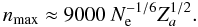 (30)Here, the mean radius of an atom ⟨ r ⟩ nl was estimated for the orbital quantum number l = 0. The occupation probability quickly decreases with n for a given value of the electron density Ne. From Eq. (18) one can obtain
 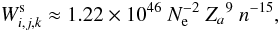 (31)as far as βi,j,k < 1. This indicates that the occupation probability decreases by several orders of magnitude for levels between n′ to nmax, viz.
 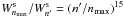 and effective truncation of the partition functions takes place due to decrease of the occupation probability of levels before the largest atomic orbit with nmax has the tendency to extend beyond the nearest ion. For
  , one can find
 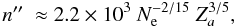 (32)which is near to Kurucz’s empirical formula for cutoff energy levels in opacity calculations.
In addition to the static perturbations of radiated atoms (ions) described above, inelastic collisions of radiated atoms (ions) with electrons should be considered for energy levels with high values of n. In the Hummer & Mihalas (1988) model of such collisions the probability that the level is bound can be expressed as ![Mathematical equation: \begin{equation} W_{n}^{\rm{c}} = \exp \left[ - 4.84 \times 10^{-17} ~ N_{\rm{e}} n^6 {{Z}_{a}}^{-4} f_{n}({{Z}_{a}}, T) \left/ \left( 1 - \left(\frac{n}{n^{\rm{c}} + 1}\right)^{2} \right)\right. \right]. \end{equation}](/articles/aa/full_html/2012/11/aa19168-12/aa19168-12-eq152.png) (33)We interpolate fn(Za,T) and nc functions tabulated by Hummer & Mihalas (1988) to the input parameters Ne, T and Za assuming that the values of fn(Za = 8,T) and nc(Za = 8) can be used whenever Za ≥ 8. As pointed out by Hummer & Mihalas (1988), the model is not well defined for very high values of n and we simply put
(33)We interpolate fn(Za,T) and nc functions tabulated by Hummer & Mihalas (1988) to the input parameters Ne, T and Za assuming that the values of fn(Za = 8,T) and nc(Za = 8) can be used whenever Za ≥ 8. As pointed out by Hummer & Mihalas (1988), the model is not well defined for very high values of n and we simply put  in Eq. (33) if n ≥ nc.
For cool and high-density plasma collisions between neutral atoms may be important. Again, following Hummer & Mihalas (1988), the occupation probability can be approximated as ![Mathematical equation: \begin{equation} W_{i,j=0,k}^{\rm{n}} = \exp \left[ - \frac{4 \pi}{3} \Sigma_{j=0,k'} N_{j=0,k'} ( r_{i,j=0,k} + r_{1,j=0,k'} ) ^{3} \right]. \end{equation}](/articles/aa/full_html/2012/11/aa19168-12/aa19168-12-eq161.png) (34)Here, j = 0 means neutral atoms, ri,j = 0,k the radius of the radiated atom k at state i, while r1,j = 0,k′ corresponds to the radii of perturbed atoms k′ at the ground state with densities Nj = 0,k′.
(34)Here, j = 0 means neutral atoms, ri,j = 0,k the radius of the radiated atom k at state i, while r1,j = 0,k′ corresponds to the radii of perturbed atoms k′ at the ground state with densities Nj = 0,k′.
Assuming that the static and dynamic perturbations are essentially independent, we use the product of  to calculate the probability that the level is occupied. The last factor is equal to 1.0 for ionized species (j ≠ 0). In stellar atmospheres with the solar abundance of elements discussed in this paper,
  and
and  are close to unity for low and moderate values of n, and it is sufficient to use only the function of
  . For lower densities, however, both n′ and nmax are high and the model of inelastic collisions could be considered. As supposed by Hummer & Mihalas (1988), it can influence the internal partition functions of elements. Collisions between neutral atoms may be important for cool plasma with a high density of neutral species.
We used the occupation probability formalism described above to calculate partition functions from neutral atoms to hydrogenic ions of the following elements: H–Si, S, Ar, and Ca. The necessary atomic data were taken from the OP TOPbase website6, where models of atoms with electron configurations up to n = 10 are available. The quantum defect description of states was applied for levels with higher values of n, up to nmax. In the OP TOPbase project extensive atomic data are also available for the ions of Fe III–Fe XXV, while one can find Fe II, Ti XX, Cr XXI, and Ni XXVI in the OP TIPbase project. Moreover, some ions of other elements (Sc–Ni) one can also find in the OP TIPbase website7. The atomic data at OP TIPbase are not as rich as for species from the OP TOPbase. Therefore we used the partition functions computed by Kurucz in 1988 that were recently updated to the ATLAS codes for the iron group elements: Sc I–IX, Ti I–IX, V I–IX, Cr I–IX, Mn I–IX, Fe I–IX, Co I–IX, Ni I–IX, and Cu I–IX. As mentioned above, these data include sufficiently high ionization stages to obtain ion populations up to T ≈ 200 000 K.
The occupation probability formalism also affects the spectroscopic properties of the plasma. According to Hubeny et al. (1994), the absorption coefficient at a frequency ν of an atom in state i is given by ![Mathematical equation: \begin{equation} \chi_{i}(\nu) = N_{i}{} \left[ \Sigma_{i' > i} W_{i',j,k} \sigma_{ii'}(\nu) + \sigma_{ic} ^{\rm{tot}} (\nu) \right] \left(1 -{\rm e}^{- h \nu / k T}\right). \end{equation}](/articles/aa/full_html/2012/11/aa19168-12/aa19168-12-eq174.png) (35)To a good approximation
(35)To a good approximation  (36)for bound-bound transitions, where fii′ is the oscillator strength and φii′(ν) the normalized profile of the absorption coefficient. For bound-free transitions one can use
  (37)and
 ![Mathematical equation: \begin{equation} \sigma_{ic} ^{\rm{tot}} (\nu) = [ 1 - W^* (n^*) ] \sigma_{ic} ^* (\nu) ~ ~ ~ {\rm{if}} ~ ~ ~ \nu < \nu_{ic}. \end{equation}](/articles/aa/full_html/2012/11/aa19168-12/aa19168-12-eq179.png) (38)Here, νic is the ionization frequency for the unperturbed atom and W ∗ (n ∗ ) corresponding to the effective quantum number
(38)Here, νic is the ionization frequency for the unperturbed atom and W ∗ (n ∗ ) corresponding to the effective quantum number  (39)designates the highest level that can be reached from the state of i with the principal quantum number n by absorption of a photon of energy hν. We calculate W ∗ (n ∗ ) by interpolating the occupation probability Wi,j,k of levels i to the effective quantum number n ∗ .
  is the extrapolated photoionization cross-sections σic(ν) to the lower frequency side of the ionization limit νic.
The absorption coefficient χi(ν) given by Eq. (35) is corrected for the stimulated emission and can be used under LTE conditions. The first term in Eq. (35) corresponds to the bound-bound transitions at frequency ν from the level of i to the undissolved (bound) part of the state i′, which occurs with the probability Wi′,j,k. The second term represents the bound-free transitions. Equation (36) refers to the “true” transitions between undissolved parts of the levels of i and i′, while the transitions between the undissolved to the dissolved components of the levels i and i′ are included in Eq. (35) with  given by Eq. (38). The transitions from the dissolved part of i to higher levels and the true free-free transitions are already included in the free-free opacities. We note that the formulae (35)–(38) differ from those used by Däppen et al. (1987) and Bergeron et al. (1991). How this influences the opacities for line transitions between low and high excited levels is discussed in Sect. 4.
There are several slightly different MHD-type occupation probability functions used in the literature. In addition to the post-Holtsmark distribution function used by Hubeny et al. (1994), Nayfonov et al. (1999), and Tremblay & Bergeron (2009), the true Holtsmark distribution, which gives  , was assumed for studying white dwarfs by Bergeron et al. (1991). A simplified approximate form of the Holtsmark microfield for randomly distributed ions was introduced by Hummer & Mihalas (1988) to reduce the computational effort for the free energy of the gas. The resulting occupation probability function, denoted here as
  , corresponds to the nearest-neighbor theory (cf. Unsöld 1948) but includes an additional empirical factor, which results in
  , whenever
  . This approximate function was used by Seaton et al. (1994) to calculate OP EOS and OP opacities.
There is, however, a problem of consistency of line profiles and the occupation probability function used for hydrogen as first pointed out by Seaton (1990), cf. also Bergeron (1993). The commonly accepted theory describing these line profiles is the unified theory of Stark broadening elaborated by Vidal et al. (1970, 1971, 1973), cf. also Lemke (1997), where a grid of hydrogen profiles are available. This theory is valid for the entire line profile from the impact regime in the core to the quasi-static far wings. To improve the consistency of the line profiles with the true Holtsmark or post-Holtsmark distributions used to calculate the occupation probability functions, one can use the function of  with the additional factor of 2 introduced to the argument of the post-Holtsmark distribution, cf. Bergeron (1993) and Hubeny et al. (1994). This approximation applies only to hydrogen, assuming that both protons and electrons contribute to the profile equally. Another approach, originally proposed by Seaton (1990), uses
  , as in Hummer & Mihalas (1988) or
  as in Nayfonov et al. (1999), with line profiles renormalized in such a way that only electric microfields β with an amplitude inferior to the critical field βi′,j,k for the upper level i′ of the transition contribute to the broadening of the lines by the protons. Another renormalization of line profiles was proposed by Tremblay & Bergeron (2009) for atmospheres of white dwarf stars.
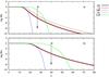 |
Fig. 3 Panel a) The occupation probability function Wn (in logarithmic units) for the bound states of H I with the principal quantum number n for a typical physical parameters at τR ≈ 0.2 of a model of Teff = 25 000 K and lgg = 4.0. Explanation of the functions displayed is given in the text. Panel b) The same as panel a), but for He II. |
Figure 3 shows MHD-type probability functions of  (marked as H lines),
  (pH lines),
  (HL line), (HM lines), together with (Coll lines), respectively, for a model of Teff = 25 000 K and lgg = 4.0 at τR ≈ 0.2, where lgNe ≈ 14.4. Clearly, the two Holtsmark-type distribution functions, and , are almost the same, but their simplified approximate form, , decreases with n much more sharply. Similarly, the two types of collisions described above result in sharp cutoff level populations, but for higher values of n. In all cases considered above, an effective truncation of the partition functions takes place due to decrease of the occupation probability of levels before the largest atomic orbit with nmax has the tendency to extend beyond the nearest ion, and before the above-mentioned theory of lowering of the ionization energy (Eqs. (13) and (14)) relaxes levels as unbounded ones. In Fig. 3 we also plot the Kurucz cutoff energy levels.
3.2. Bound-free transitions for metals
In ATLAS12/MHD-Q, bound-free transitions for metals (Z > 2) can be calculated either as in the original ATLAS12 code distributed by Kurucz or for large-scale data given by the OP/IRON project. The latter, available from the TOPbase at CDS (Cunto et al. 1993) or the XSTAR (Bautista & Kallman 2001) atomic databases, include detailed photoionization cross-sections with extensive resonance structures for all energy levels of bound states with n ≤ 10 and l ≤ 7. We used resonance-averaged photoionization cross-sections (cf. Bautista et al. 1998) for more than 1000 bound states of atoms and ions of C through Si (Z = 6−14), S (Z = 16) and Fe (Z = 26).
3.3. Bound-bound transitions
All bound-bound transitions for metals were calculated assuming the Voigt function with the natural, Stark, van der Waals, and thermal broadening of the line absorption coefficients. The broadening parameters are taken from Kurucz’s atomic base.
Detailed cross-sections tabulated by Lemke (1997) or by Shoening & Butler (after Hubeny & Lanz 2000) are implemented in the ATLAS12/MHD-Q code for H I bound-bound transitions. These profiles include the convolution of the Stark and thermal Doppler profiles. The approximate Stark broadening given by Peterson (after Kurucz 1970) or by Hubeny et al. (1994) as well as the procedure of HPROF4 developed by Peterson for the Stark effect of hydrogen lines included in the original ATLAS12 code can also be used.
Similarly, detailed profiles of selected He I lines given by Barnard et al. (1974, 1975) and Griem (1972), as well as profiles for the Balmer, Pashen and Pickering series of He II calculated by Schoening & Butler (1989a,b) are implemented. Helium lines can be also calculated under the assumption of the Voigt function or profiles with the approximate Stark broadening given by Hubeny et al. (1994).
3.4. ATLAS/OP code
ATLAS/OP is designed for computing LTE model atmospheres using monochromatic opacity and EOS data taken from the OP project distributed as the OPCD v. 3.3 base, cf. Seaton (2005). This OP base includes monochromatic cross-sections of the 17 most abundant elements (cf. Sect. 2) calculated for the temperature range of lgT = 3.5−8.0 with the step of 0.05 dex. The second parameter, lgNe, is in the range specified for each value of lgT with the step of 0.5 dex. The OPCD base also contains several computer codes for calculating the Rosseland (and Planck) mean opacities as well as mass-densities for chemical compositions specified by the user. The accurate calculations of the Rosseland-mean opacities are made for equally-spaced points in the variable v, viz.:  (40)where
 ![Mathematical equation: \begin{equation} v(u) = \int_{0}^{u} \frac{F(u)}{[1 - \exp(-u)]} {\rm d} u \end{equation}](/articles/aa/full_html/2012/11/aa19168-12/aa19168-12-eq217.png) (41)and σR is the Rosseland-mean cross-section in atomic units (
(41)and σR is the Rosseland-mean cross-section in atomic units ( ). The function of F(u) is given by Eq. (3) and the total cross-section, σ, for a mixture of elements with fractional abundances fk is
 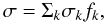 (42)where cross-sections σk are given in atomic units and include the true absorption (not corrected for stimulated emission) and scattering cross-sections (divided by the stimulated emission factor). The Rosseland-mean opacity per unit mass (κR) is equal to
  (43)where μ is the mean atomic weight. Finally, the resulting lgκR and its derivatives are interpolated to the input values of lgT and lgρ using bi-cubic interpolations.
With the exception of H and He, monochromatic opacities σk are stored in the OPCD v. 3.3 base at 10 000 variably spaced points of the variable u from 0.073157 to 20. (For H and He another u-mesh points are used.) Of course, data for different values of lgT do not correspond to the same wavelength points. This does not matter for calculations of the Rosseland (and Planck) mean opacities for the fixed set of (lgT, lgNe)-values and then interpolation to the input parameters of temperature and density. However, we need the radiation field at wavelength points simultaneously covering cool (optically thin) and hot (optically thick) regions, where T is changing by a factor of about 4. In the ATLAS/OP code we therefore added ATLAS opacities for the continuum at wavelength points outside the range of OPCD v. 3.3 data.
In the ATLAS/OP code we made bi-cubic interpolations of the total OP cross-sections for a given mixture of elements (corrected for scattering and stimulated emission) to the input parameters of lgT and lgρ. The interpolations of monochromatic opacities was performed in exactly the same manner as the original OP codes do for the Rosseland- and Planck-mean opacities.
As mentioned above, OP monochromatic data must also be interpolated to fixed wavelength points appropriate for the assumed Teff. This can be performed either by interpolating the total opacities σ or individual opacities of each element σk (cf. Eq. (42)) to fixed wavelength points. The results are not the same due to the intermediate spectral resolution of the OP data used. Interpolations of the individual monochromatic opacities of each element, σk, to the needed wavelength points and then summing the total cross-section σ gives more accurate results.
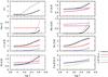 |
Fig. 4 The internal partition functions (in logarithmic units) vs. lgT for ATLAS12/MHD-Q model of Teff = 15 000 K and lgg = 4.0 (thick lines) in comparison with Kurucz’s data shown as thin lines. The panels show H I, He I and II, and the first three ionization stages of C, N, O, Ne and Si, respectively. The lowest right-hand panel shows the same, but for Fe III–V. The ionization states of I–V are plotted by means of lines as explained in the right-hand side of the figure. |
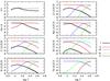 |
Fig. 5 The ionization fractions (in logarithmic units) of species for the same models as in Fig. 4. Symbols used are the same as in Fig. 4. |
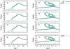 |
Fig. 6 Panel a) The Rosseland-mean opacities, κR [cm2 g-1] , as a function of lgT for ATLAS12/MHD-Q (dotted line) in comparison with OP (continuous line) and OPAL (dashed line) envelope models of Teff = 25 000 K and lgg = 4.0. Panel c) The same as panel a), but OP/IRON bound-free absorptions of metals are included in the ATLAS12/MHD-Q model (dotted line). Panel e) The same as panelc), but OP opacities are used for hydrogen and helium. Panel g) The same as panel a), but the ATLAS12/OP model is plotted by means of an A/OP line. The right-hand side panels show the same as the left-hand side ones, but for the diagrams of κR vs. lgR. |
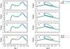 |
Fig. 7 Same as Fig. 6, but for |

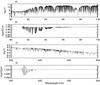 |
Fig. 8 Panel a) Emerging flux of radiation, H [erg cm-2 s-1 nm-1] , near the Lyman series of H I for the ATLAS12/MHD-Q model of Teff = 25 000 K and lgg = 4.0. Panel b) The ratio of the emerging fluxes for models calculated with different description of the occupation probability formalism (see text). Panel c) The same as panel a), but for the Balmer series of H I. Panel d) The same as panel b), but for the Balmer series of H I. |
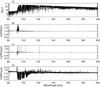 |
Fig. 9 Emerging flux of radiation, H [erg cm-2 s-1 nm-1] , near the Lyman series of H I (panel a)) of the model of ATLAS12/MHD-Q shown in Figs. 6a and b is compared with models calculated with the ATLAS/PFK code with different profiles for H I, He I and He II line absorption coefficients (see text). |
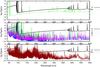 |
Fig. 11 OP monochromatic cross-sections (in atomic units) of H, He, C, N, O and Fe elements for lgT = 4.35 K and lgNe = 15.0 corrected for abundance parameters of the elements, σkfk. Panel a) shows the cross-sections for H (thick line) and He (dashed line). Panel b) shows data for C, N and O elements in comparison with the dominant absorber of H. Panel c) shows the same as panel b), but for Fe. |
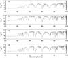 |
Fig. 12 Emerging flux of radiation, H [erg cm-2 s-1 nm-1] , near the Lyman series of H I for ATLAS/OP models shown in panels a) − d) for (Teff,lgg) = (20 000, 4.5), (28 000, 4.5), (250 000, 4.0), (25 000, 5.0), respectively. |
4. Results
4.1. LTE models of stellar atmospheres with the occupation probability formalism
Figure 4 shows examples of the internal partition functions, Uj,k, calculated in terms of the occupation probability formalism taking into account both the static and dynamic perturbations of species in comparison with the Kurucz data. The static perturbations were calculated for the post-Holsmark microfield of randomly distributed ions, while the dynamic perturbations caused by inelastic collisions of radiated atoms (ions) with electrons and collisions between neutral atoms were calculated as described in Sect. 3.1. Clearly, large differences are present for H I (U0,1). In this case, however, hydrogen is markedly ionized and only a weak effect is seen on EOS. For other species, significant differences exist at optically thick layers. Note, however, the very good agreement of our results with partition functions calculated by Kurucz (cf. Sect. 3.1) for Fe III–V, as Fig. 4 illustrates. The same is true for Fe VI–IX. We found a similar behavior of the partition functions for all models of B stars. For H I, discrepancies decrease with lower values of Teff and become small for Teff ≈ 10 000 K, where the exponent factor in Eq. (10) is able to effectively cut off occupations of high levels, cf. Sect. 3.1. The partition functions shown in Fig. 4 have indeed only weak effect on the ionization fractions of He and metals for B stars, as Fig. 5 shows for the same model of Teff = 15 000 and lgg = 4.0. The truncation effect in the partition functions remains significant only for the ionization fraction, Nj,k/ΣjNj,k, of H I and cancels exactly when the ratio of Nj,k/Uj,k (cf. Eq. (11)) is computed. For He and metals, differences arise for higher values of temperature and density. Quantitatively, this also depends on the MHD-type occupation probability function used. The ionization fractions generated by the ATLAS12/MHD-Q code with the  function (cf. Sect. 3.1) agree well with Mihalas et al. (1988, 1990) results for very broad physical conditions. This means that both the Saha-type equation of state (cf. Kurucz 1970; Mihalas 1978) implemented by the occupation probability functions and the MHD-type equation of state, which is based on the minimization of the free-energy of gas, give the same results for much broader physical parameters than studied in this paper. More details will be given in a future paper, where properties of stellar envelope models will be discussed.
Figures 6 and 7 show the diagrams κR vs. lgT and κR vs. lgR for models calculated with the ATLAS12/MHD-Q, ENV/OPAL, and ENV/OP codes for Teff = 25 000 and 45 000 K, respectively. Chemical mixtures corresponding to X = 0.708 and Z = 0.0172 were used, cf. Table 1. The ATLAS12/MHD-Q models shown in these figures were calculated with an opacity sampling (OS) approach implemented by MHD-Q formalism assuming  for the occupation probability of levels. Atomic data of LOWLINES.DAT, HIGHLINES.DAT and GFALLNLTE.DAT taken from the Kurucz website were used for metals. In panels a and b, H I, He I and He II profiles tabulated by Schoening & Butler (after Hubeny & Lanz 2000), Griem (1972) and Schoening & Butler (1989a,b), when available, were used, otherwise approximate profiles given by Hubeny et al (1994) were assumed. Photoionization cross-sections from the original ATLAS12 code were used. Panels c and d show the same, but OP/IRON photoionization cross-sections (cf. Sect. 3.2) were used. ATLAS12/MHD-Q models calculated with total OP cross-sections of H and He and OP/IRON photoionization cross-sections for metals are shown in panels e and f. Finally, models calculated with the ATLAS12/OP code (cf. Sect. 3.4) are plotted in panels g and h. In Fig. 7g we also plot the Castelli & Kurucz (2003) model. Evidently, this model predicts a high opacity excess near lgT ≈ 5.06, which reflects differences in the atomic bases for bound-bound transitions for metals and possibly the effect of splitting the LS terms into individual total angular momentum J-levels for autoionizing transitions, cf. Sect. 1, instead of treating each LS term as a whole as in the OP cross-sections.
As mentioned above, the ATLAS12/MHD-Q emerging fluxes of radiation presented in this paper were taken from the last iteration during construction of the models. (In the last few iterations, high spectral resolution was used, taking into account 1.2 million wavelength points.) Figures 8–10 show examples of emerging flux of radiation near the limits of the H I Lyman and H I Balmer series. The behavior of the theoretical spectra at these regions is dominated by hydrogen line opacities and, in principle, it offers the possibility of studying the occupation probability formalism discussed in Sect. 3.1 in astrophysical conditions. In particular, Fig. 8a shows the emerging flux of radiation near the Lyman series of H I for the model of Teff = 25 000 K and lgg = 4.0 assuming that the hydrogen absorption coefficients are given by Eqs. (35)–(38) with for occupation probability functions. Figure 8b illustrates how models are affected by the function of and Däppen’s et al. (1987) approach to line absorption coefficients mentioned in Sect. 3.1. Panels c and d of Fig. 8 show the same, but near the Balmer limit. This clearly influences the emerging spectra only near the Lyman and Balmer limits.
Now, we illustrate how the approximate profiles of H I, He I and He II affect atmospheric models of B stars. Figures 9 and 10 show the comparison of emerging fluxes of radiation for models constructed using the ATLAS12/MHD-Q and ATLAS12/KPF (cf. Sect. 3.1) codes. The former flux denoted as H is shown in panels a; the others are denoted as H(PFKx). We extended the partition functions of the ATLAS12/KPF code to all ions of species up to Z = 28 to obtain more consistent models at great optical depths. This happens only for highest ionization states of species, which are not present in the original code. We assumed that these missing partition functions can be approximated by the values of statistical weight of the ground states of the considered ions. The flux ratio of H(KPFf)/H is shown in panels b for the case when the same hydrogen and helium cross-sections, taken from ATLAS12/MHD-Q, were used in both codes. Panels c correspond to H(KPFd) with the Stark broadening of H I lines following the Kurucz (1970) and Voigt function for helium lines. Panels d shows the same as panel c, but the emerging flux H(PFKe) corresponds to the model calculated with the HPROF4 procedure for H I (cf. Sect. 3.3). As one can see, the results based on ATLAS12/KPF code with approximate cross-sections for H I, He I and He II differ markedly from those of corresponding to ATLAS12/MHD-Q model. It significantly affects the emerging flux distribution and the energy balance of the atmosphere. The former effect is of considerable importance if the models are to be employed in a subsequent analysis of stars. The latter effect changes the structure of the atmospheric model itself and hence the line profiles of H I, He I and He II, as well as metals, especially in UV range. It can to some degree influence the derived abundances and turbulent velocities from observed spectra of stars.
4.2. Examples of LTE models with OP monochromatic opacities and OP EOS for B stars
Figure 11 shows examples of OP monochromatic cross-sections, σk, corrected for abundance parameters fk of the elements taken from the last column of Table 1 (cf. Eq. (42)) for lgT = 4.35 K and lgNe = 15.0. The panels a−c display He, C–O and Fe in comparison with the dominant absorber of H (thick line), respectively. We note that some narrow lines can be missing for a given value of T due to moderate resolution in u. Other lines can appear when T is changing by 0.05 dex. as in the OPCD v 3.3 data. Better sampling over T and u is necessary to improve the quality of the data. In practical applications, however, this mainly influences synthetic spectra, but structures of atmospheric models are not influenced very much because very high spectral resolution is not necessary to calculate the total flux of radiation integrated over frequency with a good accuracy. Indeed, Figs. 6 and 7 show that the ATLAS/OP models fit the internal structure of stars calculated with the ENV/OP code well. This does not mean, however, that emerging spectra are able to fit observed high-resolution spectra of stars with a good accuracy. In addition to moderate sampling over u, T and Ne of OP data used, there is also a problem connected with the fact that wavelengths of bound-bound transitions are known only approximately because of the model atoms used in the OP/IRON project. An example is well illustrated in Fig. 12, where the C III line is located at λ ≈ 96 nm instead of λ ≈ 97.7 nm.
Moreover, the OP project (and the OPCD v. 3.3 base) includes spectral lines only for transitions in which the final state has an effective quantum number of  , where
  or
or  whenever the effective quantum number of an initial state is
  or >5, respectively, viz., all levels with
  are assumed to be fully dissolved, cf. Seaton et al. (1994). This effect is clearly seen in Figs. 12 and 13, where the Lyman and Balmer series of H I are plotted. A more careful examination of Fig. 12 reveals that the pseudocontinuum of He II extends from the ionization limit to about 97.8 nm.
Despite these limitations, the continuum level of energy fluxes of radiation agrees well with the ATLAS12/MHD-Q models, cf. Figs. 8, 12 and 13.
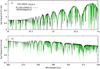 |
Fig. 14 Panel a) Emerging flux of radiation, lgH, near the Lyman series of H I for the ATLAS12/MHD-Q and BG25000g400v2.uv.7 models, respectively. Panel b) The same as panel a), but near the Balmer limit of H I. |
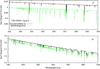 |
Fig. 15 Same as Fig. 14, but near the line series of He I, He II and the Paschen limit of H I (panel b)). |
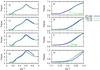 |
Fig. 16 Rosseland-mean opacities, κR [cm2 g-1], vs. lgT for LTE (dotted lines) and non-LTE (dashed lines) models calculated with the TLUSTY200 computing code for Teff = 25 000 K and lgg = 4.0 with different mixtures of elements compared with the ATLAS12/MHD-Q models (thick lines). The chemical compositions of elements are the following: H+He (panels a) and b)), H–Ca (panels c) and d)), H+He+Fe (panels e) and f)) and all elements considered in the codes (panels g) and h)). The right-hand side panels display the same models as the left-hand side ones, but only the outermost layers are shown. |
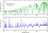 |
Fig. 17 Panel a) Emerging fluxes of radiation, lgH, near the Lyman limit of H I from LTE (dashed line) and non-LTE (continuous line) models calculated with the TLUSTY200 computing code including H–Fe species. Panels b) The ratio of the spectra shown in panel a). |
4.3. Remarks about non-LTE models
In this section some additional remarks about non-LTE models of atmospheres are made in the context of the aim of this paper. The LH models of B-type stars (Lanz & Hubeny 2007) explicitly include 46 ions of H, He, C, N, O, Ne, Mg, Al, Si, S, and Fe that are represented by about 53 000 individual levels grouped into 1127 superlevels. Line opacity includes about 39 000 lines of elements from H to S and many more lines of Fe dynamically selected from a list of about 5.65 million lines taken mainly from the Kurucz atomic base. Despite this, the LH models underestimate stellar opacities, as discussed in Sect. 2. How this influences the emerging flux of radiation is illustrated in Figs. 14 and 15, where the ATLAS12/MHD-Q data are compared with synthetic spectra calculated by Lanz & Hubeny that are distributed for general use through the TLUSTY website (cf. Sect. 1).
Clearly, there is a quantitatively similar behavior of H I lines near the Lyman limit (cf. Fig. 14a) in agreement with the fact that both models use the same occupation probability formalism for H I lines. Note that of the markedly lower continuum level of the LH spectrum in comparison with the ATLAS12/MHD-Q, however. The same is true for the spectral region in which the Balmer lines are present, cf. Fig. 14b.
Figure 15a displays the wavelength regions near the ionization limit of the He I line series. This ionization limit is clearly seen in the BG25000g400v2.vis.7 spectrum (lower curve in panel a) calculated by Lanz & Hubeny. Again, the upper spectrum corresponds to the ATLAS12/MHD-Q model. As mentioned above, the occupation probability formalism was implemented in ATLAS12/MHD-Q code not only for hydrogen but also for other species and then used in calculations of the stellar monochromatic opacities and the equation of state. Finally, Fig. 15b shows the wavelength region near the Paschen limit of H I populated by He I and He II line series.
It is also interesting to compare models of atmospheres calculated with the ATLAS12/MHD-Q and TLUSTY200 codes for individual chemical species. Examples of such a comparison are given in Fig. 16, where models included only H−He, H−Ca, H+He+Fe and all absorbers considered in the codes are shown. All species up to Z = 30 are always included in the evaluation of the equation of state. As one can see in Fig. 16, the Rosseland-mean opacities obtained from ATLAS12/MHD-Q code are higher than those obtained from the TLUSTY200 code. Generally, differences increase when metallic atoms are added to the calculations, but note the fairly good agreement between models that include absorption caused by exactly the same elements, cf. panel c of Fig. 16, where H, He and Fe only are included in the two codes. We conclude that more attention should be given to model atoms of C–Ca in calculations of non-LTE models. These elements contribute significantly to stellar opacity and play a dominant role in cooling the outermost layers of atmospheres (cf. panels b and d of Fig. 16).
A deeper insight into the problem follows from a comparison of LTE and non-LTE models calculated with the TLUSTY200 code with the same input parameters. The results are shown in Figs. 17 and 18. In both cases the spectra were taken from the last iteration during the constructions of the models. Evidently, the non-LTE effects are much weaker than Figs. 14 and 15 suggest. The ratio of non-LTE to LTE spectra plotted in panels b indicates that non-LTE effects are important for spectral lines (especially in the UV range) while only weak effects are present in the Balmer, Paschen, etc. continuum levels.
As pointed out by Lanz & Hubeny (2007), there are still several points that are only crudely approximated. Some of them result from the present lack of sufficient atomic data, but some of them might require constructing more detailed model atoms, or possibly also splitting some superlevels into individual levels. On the other hand, there are many parameters in the TLUSTY200 code with default values recommended by Hubeny & Lanz. Many of them are the result of a compromise between computer time, computer memory, etc. and the physics of the problem. These parameters can be verified by users when new models are calculated.
We also calculated LTE and non-LTE models using the TLUSTY200 computing code with an extended list of model atoms. In particular, Fig. 1 shows the effect of the increasing number of O V levels from 6 (as in LH models of B stars, cf. Lanz & Hubeny 2007) to 40 levels (as in LH models of O stars, cf. Lanz & Hubeny 2003). Adding Mg I, P IV–P V, S VI, Fe VI, Ni V, and Ni VI ions and changing the default parameters, that control the width of lines to improve coverage of the frequency interval corresponding to some bound-bound transitions improves the agreement with the ATLAS12/MHD-Q models, but it does not entirely solve the problem pointed out in Sect. 2. The lack of less abundant elements in the LH-type models possibly plays an important role. We plan to investigate non-LTE models in a more detailed manner in a future paper.
5. Conclusions
We quantitatively compared LTE and non-LTE models of atmospheres with stellar envelope structures calculated for OPAL and OP data. An inspection of the published models of atmospheres (Castelli & Kurucz 2003; Lanz & Hubeny 2003, 2007) revealed systematic differences between them and with envelope models for early-type stars (cf. Sect. 2). The Castelli & Kurucz (2003) models show a high excess of opacity at the bottom of the photospheres of hot stars. If the Castelli & Kurucz models are correct, the new opacity bump at lgT ≈ 5.06 should be considered in addition to the opacity bumps at lgT ≈ 4.6 (dominated by hydrogen and helium lines) and lgT ≈ 5.3 (the main metallic opacity bump, which plays a crucial role in stellar oscillations). It should be noted, however, that the opacity bump at lgT ≈ 5.06 does not occur either in the Lanz & Hubeny models or in the newly calculated models presented in this paper. It is clear that non-LTE models calculated by Lanz & Hubeny underestimate stellar opacities.
We calculated new LTE models of atmospheres (denoted as ATLAS12/MHD-Q) with the modified ATLAS12 computing code distributed in a basic version by Kurucz. The major modifications are the implementation of the occupation probability formalism (cf. Sect. 3.1) and the OP/IRON photoionization cross-sections (cf. Sect. 3.2). The occupation probability formalism is important for two aspects: the stellar monochromatic opacities near ionization limits of line series and the equation of state. All atomic data needed to calculate the equation of state were taken from the OP TOPbase project. Partition functions of all ions were calculated for the following elements: H−Si, S, Ar, and Ca. For iron group elements, Sc−Cu, we used the data recently updated by Kurucz, which include ionization stages from I to IX. Partition functions for higher ions of Fe were calculated using OP TOPbase atomic data. We found that both the Saha-type equation of state with the partition functions implemented by the occupation probability functions and the MHD-type equation of state give the same results for the ionizations fractions and thermodynamic variables in a broad range of physical parameters. In models studied in this paper, the ATLAS/KPF (cf. Sect. 3.1) gives almost the same results. Implementing the OP/IRON resonance-averaged photoionization cross-sections into the ATLAS12/MHD-Q code improves the compatibility of the atmospheric models with the internal structure of stars, but differences remain.
More complete model atoms (cf. Kurucz 2011) than used in this paper (cf. Sect. 4.1) are necessary to obtain better agreement with the CK models. Probably, the Castelli & Kurucz (2004) approach to autoionizing transitions also plays important role, as our test calculations for Fe VIII suggest.
Models based on the ATLAS/OP code fit the internal structures very well because the same opacity and EOS data were used. However, these models are unable to fit observed spectra at high spectral resolution mode. Better sampling of OP data over  , T and Ne is necessary to improve the accuracy of emerging spectra of ATLAS/OP models. Of course, synthetic spectra can be recalculated for ATLAS/OP models using a more complete list of line transitions with the best known broadening mechanisms of bound-bound transitions, as mentioned in Sect. 1. In principle, the ATLAS/OP models have an important diagnostic value for fully line-blanketed models of atmospheres and for OP data.
Concerning the above-mentioned new opacity bump at lgT ≈ 5.06, there is a suggestion from the Kurucz atomic data that the current versions of OPAL and OP opacities may need to be upgraded at least by a more complete list of bound-bound transitions and possibly by a more accurate treatment of autoionizing transitions. In terms of the OP project, this means that the splitting of spectroscopic terms of atoms into individual levels may be necessary for calculations of photoionization cross-sections with resonance structures. The new opacity bump changes markedly stellar envelope models. The well-known Fe-bump is located at lgT ≈ 5.30 in the OPAL and OP data, cf. Sect. 2. The new additional opacity bump, extracted in this paper from the Castelli & Kurucz (2003) models, is located on the outer side of the Fe-bump and therefore affects the driving zone for stellar pulsations. This markedly changes the predicted spectra of unstable oscillation modes, which will be a subject of a separate paper.
As mentioned in Sect. 4.3, we also plan to investigate non-LTE models of atmospheres in a more detailed manner in a future paper, but some conclusions and suggestions can be given here. A direct comparison of results obtained from non-LTE (e.g. Lanz & Hubeny 2003, 2007) and LTE models based on ATLAS codes (like Castelli & Kurucz 2003, or ATLAS12/MHD-Q models) can not be attributed entirely to non-LTE effects. Differences between current LTE and non-LTE models of atmospheres for B stars reflect mostly opacity differences with the exception of the outermost layers where non-LTE effects play an important role. The best way to quantitatively account for non-LTE effects is to calculate both LTE and non-LTE models with the same computing code for the same model atoms. As one can see from panels b of Figs. 17 and 18,
spectral lines are markedly affected by non-LTE effects. To study the observed energy flux distributions of stars measured in absolute units, non-LTE results should be corrected to models with a more complete treatment of the line-blanketing effect, otherwise lower values of Teff and lgg as well as higher angular diameters derived from observations in the Paschen continuum will be obtained for B stars.
We thank Kurucz for his comment on this point.
Acknowledgments
The author thanks the referee, Dr. Robert Kurucz, for helpful comments and for a critical reading of the manuscript.
References
- Badnell, N. R., Bautista, M. A., Butler, K., et al. 2005, MNRAS, 360, 458 [NASA ADS] [CrossRef] [Google Scholar]
- Barnard, A., Cooper, J., & Smith, E. W. 1974, JQSRT, 14, 1025 [NASA ADS] [CrossRef] [Google Scholar]
- Barnard, A., Cooper, J., & Smith, E. W. 1975, JQSRT, 15, 429 [NASA ADS] [CrossRef] [Google Scholar]
- Bautista, M. A. 1997, A&AS, 122, 167 [NASA ADS] [CrossRef] [EDP Sciences] [Google Scholar]
- Bautista, M. A., & Kallman, T. R. 2001, ApJS, 134, 139 [NASA ADS] [CrossRef] [Google Scholar]
- Bautista, M. A., Romano, P., & Pradhan, A. K. 1998, ApJS, 118, 259 [NASA ADS] [CrossRef] [Google Scholar]
- Bergeron, P. 1993, in NATO ASI Series 403, White Dwarfs: Advances in Observation and Theory, ed. M. A. Barstow (Dordrecht: Kluwer), 267 [Google Scholar]
- Bergeron, P., Wesemael, F., & Fontaine, G. 1991 ApJ, 367, 253 [NASA ADS] [CrossRef] [Google Scholar]
- Castelli, F., & Kurucz, R. L. 2003, IAU Symp., 210, 10 [Google Scholar]
- Castelli, F., & Kurucz, R. L. 2004, A&A, 419, 725 [NASA ADS] [CrossRef] [EDP Sciences] [Google Scholar]
- Cunto, W., Mendoza, C., Ochsebein, F. & Zeippen, C. J. 1993, A&A, 275, L5 [NASA ADS] [Google Scholar]
- Däppen, W., Anderson, L. S., & Mihalas, D. 1987, ApJ, 319, 195 [NASA ADS] [CrossRef] [Google Scholar]
- Däppen, W., Mihalas, D., Hummer, D. G., & Mihalas, B. W. 1988, ApJ, 332, 261 [NASA ADS] [CrossRef] [Google Scholar]
- Griem, H. 1974, Spectral Line Broadening by Plasmas (New York: Academic press) [Google Scholar]
- Hubeny, I. 1988, Comput. Phys. Commun., 52, 103 [NASA ADS] [CrossRef] [Google Scholar]
- Hubeny, I., & Lanz, T. 1995, ApJ, 439, 875 [Google Scholar]
- Hubeny, I., & Lanz, T. 2000, SYNSPEC – A User’s Guide, Version 43 [Google Scholar]
- Hubeny, I., & Lanz, T. 2006, TLUSTY – A User’s Guide, Version 202 [Google Scholar]
- Hubeny, I., Hummer, D. G., & Lanz, T. 1994, A&A, 282, 151 [NASA ADS] [Google Scholar]
- Hummer, D. G. 1986, JQSRT, 36, 1 [NASA ADS] [CrossRef] [Google Scholar]
- Hummer, D. G., & Mihalas, D. 1988, ApJ, 331, 794 [NASA ADS] [CrossRef] [Google Scholar]
- Hummer, D. G., Berrington, K. A., Eissner, W., et al. 1993, A&A, 279, 298 [NASA ADS] [Google Scholar]
- Iglesias, C. A., & Rogers, F. J. 1996, ApJ, 464, 943 [NASA ADS] [CrossRef] [Google Scholar]
- Kurucz, R. 1970, SAOSR, 309 [Google Scholar]
- Kurucz, R. L. 1979, ApJS, 40, 1 [NASA ADS] [CrossRef] [Google Scholar]
- Kurucz, R. 1993, CD-ROM, 13, 18 [Google Scholar]
- Kurucz, R. 1999, A&A, 200, 58 [Google Scholar]
- Kurucz, R. 2005a, Mem. Soc. Astron. It. Supp., 8, 14 [Google Scholar]
- Kurucz, R. 2005b, Mem. Soc. Astron. It. Supp., 8, 73 [Google Scholar]
- Kurucz, R. 2011, Can. J. Phys., 89, 417 [NASA ADS] [CrossRef] [Google Scholar]
- Kurucz, R., Peytremann, E., & Avrett, E. H. 1974, Blanketed Model Atmospheres for Early-Type Stars (Washington, D. C.: Smithsonian Institution Press) [Google Scholar]
- Lanz, T., & Hubeny, I. 2003, ApJS, 146, 417 [NASA ADS] [CrossRef] [Google Scholar]
- Lanz, T., & Hubeny, I. 2007, ApJS, 169, 83 [CrossRef] [Google Scholar]
- Lemke, M. 1997, A&AS, 122, 285 [NASA ADS] [CrossRef] [EDP Sciences] [Google Scholar]
- Mihalas, D. 1972, NCAR-TN/STR-76 [Google Scholar]
- Mihalas, D. 1978, Stellar Atmospheres, 2nd edn. (San Francisco: Freeman) [Google Scholar]
- Mihalas, D., Däppen, W., & Hummer, D. G. 1988, ApJ, 331, 815 [NASA ADS] [CrossRef] [Google Scholar]
- Mihalas, D., Heasley, J. N., & Auer, L. H. 1975, NCAR-TN/STR, 104 [Google Scholar]
- Mihalas, D., Hummer, D. G., Mihalas, B. W., & Däppen, W. 1990, ApJ, 350, 300 [NASA ADS] [CrossRef] [Google Scholar]
- Nayfonov, A., Däppen, W., Hummer, D. G., & Mihalas, D. 1999, ApJ, 526, 451 [NASA ADS] [CrossRef] [Google Scholar]
- Paczynski, B. 1969, AcA, 19, 1 [Google Scholar]
- Rogers, F. J., & Iglesias, C. A. 1992, ApJS, 79, 507 [NASA ADS] [CrossRef] [Google Scholar]
- Rogers, F. J., Swenson, F. J., & Iglesias, C. A. 1996, ApJ, 456, 902 [NASA ADS] [CrossRef] [Google Scholar]
- Schoening, T., & Butler, K. 1989a, A&AS, 78, 51 [NASA ADS] [Google Scholar]
- Schoening, T., & Butler, K. 1989b, A&AS, 79, 153 [NASA ADS] [Google Scholar]
- Seaton, M. J. 1987, J. Phys. B: At. Mol. Phys., 20, 6363 [NASA ADS] [CrossRef] [Google Scholar]
- Seaton, M. J. 1990, J. Phys. B: At. Mol. Phys., 23, 3255 [NASA ADS] [CrossRef] [Google Scholar]
- Seaton, M. J. 2005, MNRAS, 362, L1 [NASA ADS] [CrossRef] [Google Scholar]
- Seaton, M. J., & Badnell, N. R. 2004, MNRAS, 354, 457 [NASA ADS] [CrossRef] [Google Scholar]
- Seaton, M. J., Yan, Y., Mihalas, D., & Pradhan, A. K. 1994, MNRAS, 266, 805 [NASA ADS] [CrossRef] [Google Scholar]
- Tremblay, P. -E., & Bergeron, P. 2009 ApJ, 696, 1755 [NASA ADS] [CrossRef] [Google Scholar]
- Unsöld, A. 1948, Zs. Ap., 24, 355 [Google Scholar]
- Vidal, C. R., Cooper, J., & Smith, E. W. 1970 JQSRT, 10, 1011 [Google Scholar]
- Vidal, C. R., Cooper, J., & Smith, E. W. 1971 JQSRT, 11, 263 [Google Scholar]
- Vidal, C. R., Cooper, J., & Smith, E. W. 1973 ApJS, 25, 37 [NASA ADS] [CrossRef] [Google Scholar]
All Tables
All Figures
|
Fig. 1 Panel a) The Rosseland-mean opacities, κR [cm2 g-1] , as a function of lgT for Castelli & Kurucz (2003) (marked as CK line) and Lanz & Hubeny (2007) (LH line) models of |
| In the text | |
|
Fig. 2 Panel a) The Rosseland-mean opacities, κR [cm2 g-1] , as a function of lgT for OPAL (thick line) and OP (thin line) models of Teff = 25 000 K and lgg = 4.0. The chemical abundance parameters X = 0.708 and Z = 0.0172 are assumed. Panel b) The ratio of OP to OPAL Rosseland-mean opacities are displayed for input parameters of (lgT and lgρ) taken from the OPAL model shown in panel a). Panel c) The same as panel b), but for gas pressures. |
| In the text | |
|
Fig. 3 Panel a) The occupation probability function Wn (in logarithmic units) for the bound states of H I with the principal quantum number n for a typical physical parameters at τR ≈ 0.2 of a model of Teff = 25 000 K and lgg = 4.0. Explanation of the functions displayed is given in the text. Panel b) The same as panel a), but for He II. |
| In the text | |
|
Fig. 4 The internal partition functions (in logarithmic units) vs. lgT for ATLAS12/MHD-Q model of Teff = 15 000 K and lgg = 4.0 (thick lines) in comparison with Kurucz’s data shown as thin lines. The panels show H I, He I and II, and the first three ionization stages of C, N, O, Ne and Si, respectively. The lowest right-hand panel shows the same, but for Fe III–V. The ionization states of I–V are plotted by means of lines as explained in the right-hand side of the figure. |
| In the text | |
|
Fig. 5 The ionization fractions (in logarithmic units) of species for the same models as in Fig. 4. Symbols used are the same as in Fig. 4. |
| In the text | |
|
Fig. 6 Panel a) The Rosseland-mean opacities, κR [cm2 g-1] , as a function of lgT for ATLAS12/MHD-Q (dotted line) in comparison with OP (continuous line) and OPAL (dashed line) envelope models of Teff = 25 000 K and lgg = 4.0. Panel c) The same as panel a), but OP/IRON bound-free absorptions of metals are included in the ATLAS12/MHD-Q model (dotted line). Panel e) The same as panelc), but OP opacities are used for hydrogen and helium. Panel g) The same as panel a), but the ATLAS12/OP model is plotted by means of an A/OP line. The right-hand side panels show the same as the left-hand side ones, but for the diagrams of κR vs. lgR. |
| In the text | |
|
Fig. 7 Same as Fig. 6, but for |
| In the text | |
|
Fig. 8 Panel a) Emerging flux of radiation, H [erg cm-2 s-1 nm-1] , near the Lyman series of H I for the ATLAS12/MHD-Q model of Teff = 25 000 K and lgg = 4.0. Panel b) The ratio of the emerging fluxes for models calculated with different description of the occupation probability formalism (see text). Panel c) The same as panel a), but for the Balmer series of H I. Panel d) The same as panel b), but for the Balmer series of H I. |
| In the text | |
|
Fig. 9 Emerging flux of radiation, H [erg cm-2 s-1 nm-1] , near the Lyman series of H I (panel a)) of the model of ATLAS12/MHD-Q shown in Figs. 6a and b is compared with models calculated with the ATLAS/PFK code with different profiles for H I, He I and He II line absorption coefficients (see text). |
| In the text | |
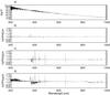 |
Fig. 10 Same as Fig. 9, but now for the emerging flux of radiation near the Balmer series of H I. |
| In the text | |
|
Fig. 11 OP monochromatic cross-sections (in atomic units) of H, He, C, N, O and Fe elements for lgT = 4.35 K and lgNe = 15.0 corrected for abundance parameters of the elements, σkfk. Panel a) shows the cross-sections for H (thick line) and He (dashed line). Panel b) shows data for C, N and O elements in comparison with the dominant absorber of H. Panel c) shows the same as panel b), but for Fe. |
| In the text | |
|
Fig. 12 Emerging flux of radiation, H [erg cm-2 s-1 nm-1] , near the Lyman series of H I for ATLAS/OP models shown in panels a) − d) for (Teff,lgg) = (20 000, 4.5), (28 000, 4.5), (250 000, 4.0), (25 000, 5.0), respectively. |
| In the text | |
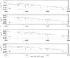 |
Fig. 13 Same as Fig. 12, but near the Balmer limit of H I. |
| In the text | |
|
Fig. 14 Panel a) Emerging flux of radiation, lgH, near the Lyman series of H I for the ATLAS12/MHD-Q and BG25000g400v2.uv.7 models, respectively. Panel b) The same as panel a), but near the Balmer limit of H I. |
| In the text | |
|
Fig. 15 Same as Fig. 14, but near the line series of He I, He II and the Paschen limit of H I (panel b)). |
| In the text | |
|
Fig. 16 Rosseland-mean opacities, κR [cm2 g-1], vs. lgT for LTE (dotted lines) and non-LTE (dashed lines) models calculated with the TLUSTY200 computing code for Teff = 25 000 K and lgg = 4.0 with different mixtures of elements compared with the ATLAS12/MHD-Q models (thick lines). The chemical compositions of elements are the following: H+He (panels a) and b)), H–Ca (panels c) and d)), H+He+Fe (panels e) and f)) and all elements considered in the codes (panels g) and h)). The right-hand side panels display the same models as the left-hand side ones, but only the outermost layers are shown. |
| In the text | |
|
Fig. 17 Panel a) Emerging fluxes of radiation, lgH, near the Lyman limit of H I from LTE (dashed line) and non-LTE (continuous line) models calculated with the TLUSTY200 computing code including H–Fe species. Panels b) The ratio of the spectra shown in panel a). |
| In the text | |
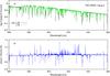 |
Fig. 18 Same as Fig. 17, but near the limit of the Balmer series of H I. |
| In the text | |
Current usage metrics show cumulative count of Article Views (full-text article views including HTML views, PDF and ePub downloads, according to the available data) and Abstracts Views on Vision4Press platform.
Data correspond to usage on the plateform after 2015. The current usage metrics is available 48-96 hours after online publication and is updated daily on week days.
Initial download of the metrics may take a while.