| Issue |
A&A
Volume 547, November 2012
|
|
|---|---|---|
| Article Number | A13 | |
| Number of page(s) | 15 | |
| Section | Stellar atmospheres | |
| DOI | https://doi.org/10.1051/0004-6361/201117506 | |
| Published online | 19 October 2012 | |
Chemically tagging the Hyades Supercluster
A homogeneous sample of F6-K4 kinematically selected northern stars⋆,⋆⋆,⋆⋆⋆
1
Dpto. Astrofísica, Facultad de CC. Físicas, Universidad Complutense de
Madrid,
28040
Madrid,
Spain
e-mail: This email address is being protected from spambots. You need JavaScript enabled to view it.
2
Instituto de Astrofísica de Canarias, C via Lactea s/n, 38200 La Laguna,
Tenerife,
Spain
3
Dept. Astrofísica, Universidad de La Laguna (ULL),
38206 La Laguna, Tenerife, Spain
Received: 17 June 2011
Accepted: 17 April 2012
Abstract
Stellar kinematic groups are kinematical coherent groups of stars that might have a common origin. These groups are dispersed throughout the Galaxy over time by the tidal effects of both Galactic rotation and disc heating, although their chemical content remains unchanged. The aim of chemical tagging is to establish that the abundances of every element in the analysis are homogeneus among the members. We study the case of the Hyades Supercluster to compile a reliable list of members (FGK stars) based on our chemical tagging analysis. For a total of 61 stars from the Hyades Supercluster, stellar atmospheric parameters (Teff, log g, ξ, and [Fe/H]) are determined using our code called StePar, which is based on the sensitivity to the stellar atmospheric parameters of the iron EWs measured in the spectra. We derive the chemical abundances of 20 elements and find that their [X/Fe] ratios are consistent with Galactic abundance trends reported in previous studies. The chemical tagging method is applied with a carefully developed differential abundance analysis of each candidate member of the Hyades Supercluster, using a well-known member of the Hyades cluster as a reference (vB 153). We find that only 28 stars (26 dwarfs and 2 giants) are members, i.e. that 46% of our candidates are members based on the differential abundance analysis. This result confirms that the Hyades Supercluster cannot originate solely from the Hyades cluster.
Key words: open clusters and associations: individual: Hyades Supercluster / open clusters and associations: individual: Hyades / stars: abundances / stars: kinematics and dynamics / stars: late-type / stars: fundamental parameters
Based on observations made with the Mercator Telescope, operated on the island of La Palma by the Flemish Community, at the Spanish Observatorio del Roque de los Muchachos of the Instituto de Astrofísica de Canarias.
Figures A.1–A.6 are available in electronic form at http://www.aanda.org
Tables A.1–A.9 and the line list and EW measurements are only available at the CDS via anonymous ftp to cdsarc.u-strasbg.fr (130.79.128.5) or via http://cdsarc.u-strasbg.fr/viz-bin/qcat?J/A+A/547/A13
© ESO, 2012
1. Introduction
Stellar kinematic groups (SKGs) – superclusters (SCs) and moving groups (MGs) – are kinematic coherent groups of stars (Eggen 1994) that could have a common origin. The youngest and most well-studied SKGs are: the Hyades SC (600 Myr), the Ursa Major MG (Sirius SC, 300 Myr), the Local Association or Pleiades MG (20 to 150 Myr), the IC 2391 SC (35–55 Myr), and the Castor MG (200 Myr) (Montes et al. 2001a). Since Olin Eggen introduced the concept of a MG and the idea that stars can maintain a kinematic signature over long periods of time, their existence (mainly in the case of the old MGs) has been disputed. There are two factors that can disrupt a MG: the Galactic differential rotation which tends to disperse the stars, and the disc heating, which causes velocity the dispersion of the disc stars to increase with age.
The overdensity of stars in some regions of the Galactic velocity UV-plane may also be the result of global dynamical mechanisms linked with the non-axisymmetry of the Galaxy (Famaey et al. 2005), namely the presence of a rotating central bar (e.g. Dehnen 1998; Fux 2001; Minchev et al. 2010) and spiral arms (e.g. Quillen & Minchev 2005; Antoja et al. 2009, 2011), or both (see Quillen 2003; Minchev & Famaey 2010). However, several works have shown that different age subgroups are situated in the same region of the Galactic velocity plane as the classical MGs (Asiain et al. 1999) suggesting that both field-like stars and young coeval ones can coexist in MGs (Famaey et al. 2007, 2008; Antoja et al. 2008; Klement et al. 2008; De Silva et al. 2008; Francis & Anderson 2009a,b; Zhao et al. 2009).
Using different age indicators such as the lithium line at 6707.8 Å, the chromospheric activity level, and the X-ray emission, it is possible to quantify the contamination by younger or older field stars among late-type candidate members of a SKG (e.g. Montes et al. 2001b; Martínez-Arnáiz et al. 2010; López-Santiago et al. 2006, 2009; López-Santiago et al. 2010; Maldonado et al. 2010). However, the detailed analysis of the chemical content (chemical tagging) is another powerful method that provide clear constraints on the membership to these structures (Freeman & Bland-Hawthorn 2002). Studies of open clusters such as the Hyades and Collinder 261 (Paulson et al. 2003; De Silva et al. 2006, 2007a, 2009) have found high levels of chemical homogeneity, showing that chemical information is preserved within the stars and that the possible effects of any external sources of pollution are negligible. This chemical tagging method has so far only been used in the three old SKGs: The Hercules stream (Bensby et al. 2007) whose stars have different ages and chemistry (associated with dynamical resonances namely a bar or spiral structure), HR 1614 (De Silva et al. 2007b, 2009), and Wolf 630 (Bubar & King 2010) the last two appear to be true MGs (debris of star-forming aggregates in the disc). In addition, Soderblom & Mayor (1993), King et al. (2003), King & Schuler (2005), and Ammler-von Eiff & Guenther (2009) studied the Ursa Major MG and demonstrated, in terms of chemical abundances and spectroscopic age determinations, that some of the candidates are consistent with being members of a MG with a mean [Fe/H] = −0.085.
The chemical tagging method has been applied to some smaller samples of possible Hyades SC members. Pompéia et al. (2011) studied a sample of 21 kinematically selected stars and identified two candidate members of the Hyades SC, whereas De Silva et al. (2011) analysed 26 southern giant candidates finding also four candidate members. These results show that the Hyades Supercluster may not originate uniquely from the Hyades cluster. In this paper, we apply the chemical tagging method to a homogeneous sample of 61 F6-K4 northern kinematically selected Hyades Supercluster (Hyades stream, or Hyades moving group) candidates most of whom are main sequence stars, although some are giant stars. In Sect. 2, we give details of our sample selection. Our observations and data reduction methodology are described in Sect. 3. Descriptions of our codes to determine the stellar parameters and chemical abundances are provided in Sect. 4. Our measurements of absolute and differential abundances are given in Sect. 5. Finally in Sect. 6, we summarize our results for the membership of the Hyades Supercluster derived from the chemical tagging method.
Identification of a significant number of late-type members of these young MGs would be extremely important for a study of their chromospheric and coronal activity and their age evolution, and could lead to a clearer understanding of the star formation history in the solar neighborhood. In addition, these stars can also be selected as targets for direct imaging campaigns to detect of sub-stellar companions (brown dwarfs and exoplanets).
2. Sample selection
The sample analyzed in this paper (see Table A.1) was selected using kinematical criteria based on the U, V and W Galactic velocities of a chosen target being within approximately 10 km s-1 of the mean velocity of the group (Montes et al. 2001a).
We also selected additional candidates and spectroscopic information about some of these stars from López-Santiago et al. (2010), Martínez-Arnáiz et al. (2010), and Maldonado et al. (2010). Some exoplanet-host star candidates were also taken from Montes et al. (2010).
After the first stage of selection based on kinematical criteria, we then eliminated stars that were unsuitable for our particular abundance analysis, namely stars cooler than K4 and hotter than F6, because for these stars we would have been unable to measure the spectral lines required for our particular abundance analysis. We also discarded stars with high rotational velocities, as well as those known to be spectroscopical binaries to avoid contamination from the companion star during the analysis.
We recalculated the Galactic velocities of our selected targets by employing the radial velocities and uncertainties derived by the HERMES spectrograph automated pipeline (Raskin et al. 2011). However, some spectra were taken when the automated radial velocity was not available, in these cases, we applied the cross-correlation method using the routine fxcor in IRAF1, by adopting a spectrum of the asteroid Vesta (as a solar reference) that had been previously corrected for Doppler shift with the Kurucz solar ATLAS (Kurucz et al. 1984). The radial velocities were derived after applying the heliocentric correction to the observed velocity. Radial velocity errors were computed by fxcor based on the fitted peak height and the antisymmetric noise, as described by Tonry & Davis (1979). The obtained radial velocities and their associated errors are given in Table A.1. Proper motions and parallaxes were taken from the Hipparcos and Tycho catalogues (ESA 1997), the Tycho-2 catalogue (Høg et al. 2000), and the new reduction of the Hipparcos catalogue (van Leeuwen 2007).
The method employed in the determination of the U, V, and W velocities is the same as that used in Montes et al. (2001a). The Galactic velocities are in a right-handed coordinated system (positive in the directions of the Galactic center, Galactic rotation, and the north Galactic pole, respectively). Montes et al. (2001a) modified the procedures of Johnson & Soderblom (1987) to perform the velocity calculation and associated errors. This modified program uses coordinates adapted to the epoch J2000 in the International Celestial Reference System (ICRS). The recalculted velocities are given in Table A.1 and plotted in the U, V, and W diagram in Fig. 1.
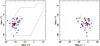 |
Fig. 1 U, V, and W recalculated velocities for the possible members of the Hyades Supercluster. Blue squares represent stars selected as members by the chemical tagging approach, red diamonds represent stars that have similar Fe abundances, but not for all the elements. Orange circles represent three Hyades cluster stars (BZ Cet, V683 Per, and ϵ Tau). Green triangles represent stars that do have similar Fe abundances (as well as similar values of other elements). The big black cross indicate the U, V, and W central location of the Hyades Supercluster (see Montes et al. 2001a). Dashed lines show the region where the majority of the young disk stars tend to be according to Eggen (1984, 1989). |
3. Observations
Spectroscopic observations (see Fig. 2) were obtained at the 1.2 m Mercator Telescope at the Observatorio del Roque de los Muchachos (La Palma, Spain) in January, May, and November 2010 with HERMES (High Efficiency and Resolution Mercator Echelle Spectrograph, Raskin et al. 2011). Using the high resolution mode (HRF), the spectral resolution is 85 000 and the wavelength range is from λ3800 Å to λ8750 Å approximately. Our signal-to-noise ratio (S/N) ranges from 70 to 300 (160 on average) in the V band. A total of 92 stars were observed. We analyzed single main-sequence and giant stars (from F6 to K4), including 61 candidates in total (including the Hyades cluster members BZ Cet, V683 Per, and ϵ Tau, see Perryman et al. 1998) and the reference used in the differential abundance analysis (vB 153). All the obtained echelle spectra were reduced with the automatic pipeline (Raskin et al. 2011) for HERMES. We later used several IRAF tasks to normalize the spectra order by order, using a low-order polynomial fit to the observed continuum, merging the orders into a unique one-dimensional spectrum and applying the Doppler correction required for its observed radial velocity. When several exposures had been performed for the same star we combined all of the individual spectra to obtain a unique spectrum with higher S/N.
4. Spectroscopic analysis
4.1. Stellar parameters
Stellar atmospheric parameters and abundances were computed using the 2002 version of the MOOG code (Sneden 1973) and a grid of Kurucz ATLAS9 plane-parallel model atmospheres (Kurucz 1993). As damping prescription, we used the Unsöld approximation multiplied by a factor recommended by the Blackwell group (option 2 within MOOG). The atmospheric parameters were inferred from 263 Fe i and 36 Fe ii lines (the iron lines and their atomic parameters were obtained from Sousa et al. 2008) iterating until the slopes of χ versus (vs.) log ϵ(Fe i) and log (EW/λ) vs. log ϵ(Fe i) were zero (excitation equilibrium) and imposing ionization equilibrium, such that log ϵ(Fe i) = log ϵ(Fe ii). However, we attempted to ensure that the [Fe/H] obtained from the iron lines matched the model metallicity. To simplify the iterative procedure, we built an automatic code called StePar that employs a Downhill Simplex Method (Press et al. 1992). The function to minimize is a quadratic form composed of the excitation and ionization equilibrium conditions. The code performs a new simplex optimization until the model’s metallicity and the iron abundance are the same. The StePar code finds the best solution in the paramater space within minutes. The obtained solution for a given star is independent of the initial set of parameters employed, hence we used the canonical solar values as initial input values (Teff = 5777 K, log g = 4.44 dex, ξ = 1 km s-1).
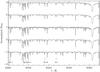 |
Fig. 2 High resolution spectra for some representative stars from our sample (from top to bottom): HD 27285 (G4 V), HD 53532 (G3 V), HD 98356 (K0 V), these three stars satisfy chemical tagging membership conditions, vB 153 (a K0 V reference star used in the differential abundances analysis) and BZ Cet (a K2 V, also member of the Hyades cluster). Lines used in the abundance analysis are highlighted on bottom. |
The uncertainties in the stellar parameters were determined as follows: for the microturbulence, we changed ξ until the slope of log ϵ(Fe i) vs. log (EW/λ) varied by an amount equal to its uncertainty (divided by the square root of the number of Fe i lines). We varied the effective temperature until the slope log ϵ(Fe i) vs. χ increased up to its own error (divided by the square root of the number of Fe i lines). By increasing ξ on its error, we recomputed the effective temperature, these two sources of error are added in quadrature.
We varied the surface gravity until the Fe ii abundance increases by a quantity equal to the standard deviation divided by the square root of the number of Fe ii lines. We also took into account the previous errors in ξ and Teff by varying these quantities separately, thus recomputing the gravity. These differences were later added in quadrature. Finally, to determine the error in the Fe abundance, we varied the stellar atmospheric parameters within their respective uncertainities, which enabled us to add all the Fe i,ii variations due to the stellar parameters uncertainities and the standard deviations of the Fe i, ii abundances in quadrature.
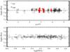 |
Fig. 3 log ϵ(Fe i,ii) versus the excitation potential, χ, and the reduced equivalent width, log (EW/λ), for the Sun (spectrum of the asteroid Vesta). The dashed lines represent the least squares fit to the data points, which are very close to a constant fit as expected from the iterative procedure of the stellar parameter determination. |
The EW determination of the Fe lines was carried out with the ARES2 code (Sousa et al. 2007). We followed the approach of Sousa et al. (2008) to adjust the rejt parameter of ARES according to the S/N of each spectrum. The other ARES parameters we employed were smoother = 4, space = 3, lineresol = 0.07, and miniline = 2.
In addition, we performed a 2-σ rejection of the Fe i and Fe ii lines after a first determination of the stellar parameters, therefore we re-run the StePar program again without the rejected lines.
As a test, we performed the parameter determination in the case of the Sun. Employing a HERMES spectrum of the asteroid Vesta with the same instrumental configuration as the other stars. In this case, we obtained: Teff = 5775 ± 15 (K), log g = 4.48 ± 0.04 (dex), ξ = 0.965 ± 0.020 (km s-1), and log ϵ(Fe i) = 7.46 ± 0.01 (dex), which are very close to the canonical solar values of the atmospheric parameters. We ended up with 220 Fe i and 27 Fe ii spectral lines for this solar reference. To illustrate this iterative procedure we present in Fig. 3 a representation of both log ϵ(Fe i,ii) vs. χ and log ϵ(Fe i) vs. log (EW/λ). In both panels of Fig. 3 the null slope is indistinguisable from the mean. In the case of Fe ii, we are only interested in its mean abundance value, which is the same as the mean abundance value obtained from the Fe i lines.
The derived stellar parameters for our solar reference are used as a zero-point. The determined abundances are presented with respect to our solar values in a self-consistent manner.
The obtained stellar parameters Teff, log g, ξ, log ϵ(Fe i), log ϵ(Fe ii), and [Fe/H] (using our solar reference) are given in Table A.2, together with the internal uncertainties in the stellar parameters. In Fig. 4, we show the histrogram distribution of Teff and log g which is also available in tabular form in the online version. The effective temperature ranges approximately from 4500 K to 6300 K. The surface gravities of most stars in the sample are those typical main sequence stars (52 out of 61), and the rest are low gravity stars.
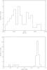 |
Fig. 4 Histograms for the determined Teff and log g of the candidate stars. |
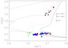 |
Fig. 5 Spectroscopic log Teff vs. log g for the candidate stars. We have employed the Yonsei-Yale ischrones (Demarque et al. 2004) for Z = 0.025 and 0.1, 0.7, 4, and 13 Gyr (from left to right). Mean error bars are represented at the middle right. Blue squares represent stars selected as members by the chemical tagging approach, red diamonds represent those stars that have similar Fe abundances, but different values of other elements. Orange circles represent three Hyades cluster stars (BZ Cet, V683 Per and ϵ Tau). Green triangles represent those stars that do not have similar Fe abundances (as well as dissimilar values of other elements). |
Elemental abundances for our solar reference (spectrum of the asteroid Vesta).
As a complementary stellar parameter test, we compiled a log g − log Teff diagram by employing the determined stellar parameters in Fig. 5. Most of the giants and the solar-like stars tend to fit within the depicted isochrones, being consisent with the isochrone for 0.7 Gyr (the accepted Hyades age, see Perryman et al. 1998). In constrast, some cooler stars tend to deviate 0.1 dex from the ischrones, particulary at the lowest temperatures. However, the mean gravity error for these cooler stars is about 0.1 dex, being compatible with the Hyades isochrone within their error bars. On the other hand, the error may be systematic, the EWs of the Fe ii lines having larger systematic errors, since they get weaker as Teff drops. This may in turn lead to an underestimation of the gravity derived assuming excitation equilibrium. The effect on the Fe ii lines may propagate as an increasing understimation of log g.
4.2. Chemical abundances
The selection of the chemical elements that we considered in this study includes those in the line list of Neves et al. (2009), which also provides the atomic parameters for each line. In addition, we considered some lines from González Hernández et al. (2010) and Pompéia et al. (2011) of some neutron-capture elements (their atomic parameters are given in Table A.9).
Chemical abundances were calculated using the equivalent width (EW) method. The EWs were determined with the ARES code (Sousa et al. 2007) following the approach described in Sect. 4.1.
Once the EWs had been measured, the analysis was carried out with the LTE MOOG code (Sneden 1973) using the ATLAS model corresponding to the derived atmospheric parameters. We determined the elemental abundances (see Tables A.3 and A.4) relative to solar values using the spectrum of the asteroid Vesta (with the same instrumental configuration) as the solar reference. These were determined by computing the mean of the line-by-line differences of each chemical element and candidate star with respect to our solar reference (see Table 1 for the solar reference elemental abundances).
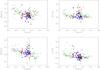 |
Fig. 6 [X/Fe] vs. [Fe/H] for the α-elements Mg, Si, Ca, and Ti: open diamonds represent the thin disc data (González Hernández et al. 2010), black upward-pointing filled triangles represent Hyades cluster data (Paulson et al. 2003), red diamonds are our stars compatible to within 1-rms with the Fe abundance but not for all elements, blue squares and blue starred symbols are the candidates selected to become members of the Hyades Supercluster (see Figs. 8, A.4, A.5, and A.6). Green downward-pointing triangles show no compatible stars. BZ Cet, V683 Per, and ϵ Tau Hyades cluster members stars are marked with orange circles. Starred points represent the giant stars. Black asterisks are the candidates selected by De Silva et al. (2011) and black crosses represent the members selected by Pompéia et al. (2011). |
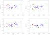 |
Fig. 8 Δ[X/H] differential abundances (for the α-elements Mg, Si, Ca, and Ti vs. Teff). Dashed-dotted lines represent 1-rms over and below the median for our sample, whereas dotted lines represent the 1.5-rms level. Dashed lines represent the mean differential abundance. Red diamonds are stars compatible within 1-rms with the Fe abundance but not for all elements, blue squares are the candidates selected to become members of the Hyades Supercluster, while green triangles are rejected candidates and starred points are the giants. Blue squares and starred points are the final selected candidates to become members of the Hyades Supercluster. BZ Cet, V683 Per, and ϵ Tau are indicated by orange circles. |
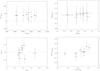 |
Fig. 10 Comparison of the stellar parameters determined with the Sousa et al. (2008) Fe i-Fe ii line list versus the list from Hekker & Meléndez (2007). |
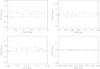 |
Fig. 11 Comparison of [X/Fe] derived with the stellar paramaters determined with the Sousa et al. (2008) Fe i-Fe ii line list versus the list from Hekker & Meléndez (2007). Dashed line represents the mean value for the differences. Dashed-dotted lines represent one standard deviation over the mean value. |
A total of 20 elements were analyzed: Fe, the α-elements (Mg, Si, Ca, and Ti), the Fe-peak elements (Cr, Mn, Co, and Ni), the odd-Z elements (Na, Al, Sc, and V) and the s-process elements (Cu, Zn, Y, Zr, Ba, Ce and Nd), see Tables A.3 and A.4. The spectral lines used and their atomic parameters were taken from Neves et al. (2009). However, to avoid incorrect EW measurements (e.g. caused by an incorrect continuum placement), we rejected lines that were separated by more than a factor two of the standard deviation (σ) from the median differential abundance derived for each line.
The differential abundances (see Tables A.5 and A.6) were also determined to establish mermbership of each candidate using a Hyades cluster member. For this purpose, we have obtained a HERMES spectrum of a well-known member of the Hyades cluster (vB 153), which is the same reference star employed in Paulson et al. (2003) and De Silva et al. (2006) in their differential analysis of the Hyades cluster. This differential treatment minimizes errors due to the uncertainities in the oscillator strengths (log gf) of each line treated in the analysis. We also computed the abundance sensitivities to changes in the stellar atmospheric parameters (see Tables A.7 and A.8). These sensitivities due to the internal uncertainties in the stellar parameters are small for all the elements (about a few hundredths of a dex) except for titanium, vanadium, barium, and zirconium, whose sensitivities to variations in the parameters is quite high (tenths of a dex).
5. Discussion
We compare our derived element abundances with those of thin disc stars (González Hernández et al. 2010) to determine whether our values follow Galactic trends. We also verify the chemical homogeneity of the Hyades Supercluster and whether some of the stars indeed have homogeneus values of all the considered elements.
5.1. Element abundances
The element abundances were determined in a fully differential way by comparing them with those derived for a solar spectrum (as stated in Sect. 4.1). The choice of elements is taken from González Hernández et al. (2010), which we also compared (see Figs. 6, 7, A.1, A.2, and A.3) with the data from Paulson et al. (2003) for the elements in common (Na, Mg, Si, Ca, Ti, and Zn). Data for those elements in common with De Silva et al. (2011) (Na, Mg, Al, Si, Ca, Sc, Ti, Cr, Mn, Co ,Ni, Zn, Ba, and Ce) and Pompéia et al. (2011) (Na, Mg, Zr, Ba, Ce, and Nd) were also added to these figures.
The α-elements (Mg, Si, Ca, and Ti) seem to follow the Galactic trends (see Bensby et al. 2005; Reddy et al. 2006; González Hernández et al. 2010), although we note that giant stars deviate in the case of Si. There is a noticable scatter in Ti and Mg, but the Ti scatter tends to increase as the [Fe/H] decreases.
For the Iron-peak elements (Cr, Mn, Co, and Ni), we find a small scatter in Ni and Cr, although the scatter in Cr increases at the lowest metallicities in this relatively narrow metallicity range as observed for Ti. For Cr, we note that most of the stars lie above the Galactic trend, and that Co has a larger scatter, and the giants tending to deviate more than the main sequence stars. In the case of Mn, there is a smaller scatter for the main sequence stars but the giants tend to deviate away from the Galactic trend. Ti may be affected by NLTE effects but as reported in (Bensby et al. 2003, and references therein) the deviations from LTE might be small if the atomic parameters are adecuate.
For the odd-Z elements (Na, Al, Sc, and V), the giant stars deviate from the Galactic trend, except for Sc. A high dispersion towards low metallicity is observed for Sc, as well as for Ti and Cr. We confirm a large dispersion for V, which some authors interpret as a NLTE effect (e.g. Bodaghee et al. 2003; Gilli et al. 2006; Neves et al. 2009). Vanadium lines are indeed difficult to measure and may require high signal-to-noise data.
The neutron capture elements (Cu, Zn, Ba, Ce, Y, Zr, and Nd) follow similar trends to those seen in solar analogs (González Hernández et al. 2010). We find some enhancement for Ba above the solar level as observed in the Hyades cluster (De Silva et al. 2006), although the scatter in the data is relatively large. This enhancement is mostly observed around Hyades-like metallicity ([Fe/H]) values. Stars of lower than solar metallicity are also enhanced in Ba, although the Galactic abundance distribution has a larger scatter below solar metallicity. Ce and Y match the Galactic pattern but at lower metallicities the stars of our sample tend to have a larger dispersion. We note here that the dispersion seen in our data is reasonable according to the quality of the data. The Zr abundance values are consistent with the abundance Galactic pattern, but those of the giants are found to deviate from the main Galactic trend. This slight deviation seen for the giants is also observed for Cu and Zn, although the dwarf stars match the Galactic trend, with the exception of Nd, which is enhanced for almost all the sample stars.
When we compare the element abundance data from Paulson et al. (2003) with our derived [X/Fe] abundances, we find that for the case of Na, Mg, Ti, and Zn some of the sample stars are consistent with the Hyades cluster abundances. However, there is an small difference for Si and a larger scatter than for Ca. These differences might be caused by the use of different line lists for these elements and the solar reference they used. Candidates obtained by Pompéia et al. (2011) are displaced about 0.10 dex in metallicity from the Hyades cluster mean value. This offset is probably caused by their different line lists and their log gf choices.
Giant stars tend to deviate from the Galactic trend in certain elements. The method presented in the present study does not seem to work for giants as well as for main sequence stars. For consistency purposes, we verified our derived stellar parameters for the giant stars. In the first place, we recomputed the stellar parameters described in Sect. 4 by using instead the iron line list of Hekker & Meléndez (2007) to investigate the origin of any possible differences. This comparison can be seen in Fig. 10, where we find an offset of ≈ 70 K compared with the results from the list of Sousa et al. (2008). The next step was to check whether the effect on the parameter determination was sufficient to explain this deviation. For this purpose, we rederived the [X/Fe] abundances making use of the set of parameters derived with the Hekker & Meléndez (2007) line list and compared them with the original [X/Fe] (see Fig. 11). As one would expect, we find systematic differences but in most cases these differences are at the level of hundreths of dex. The worst case is that of Si where the differences show an even higher [Si/Fe] abundance derived using the new set of stellar parameters. In other cases such as Mg and Ni, we find no systematic differences with a dispersion of 0.03 dex and 0.01 dex, respectively. Comparison stars from De Silva et al. (2011) (all of them are giants) also deviate from the Galactic trends in some cases and for some elements. In that article, the other metallicities of the stars considered also deviate from the Galactic trends (when compared with Bensby et al. 2005). De Silva et al. (2011) argue that Na is higher than the Galactic trend when comparing with dwarfs from the Galactic disk, perhaps owing to the internal mixing in some of the giant stars. Systematically higher Na abundances were also found for giants belonging to the Hyades cluster by Smiljanic (2012) and attributed to the internal processes operating in giant stars. This enhancement in [Na/Fe] ratio is similar to the one we found for some supercluster candidates (of about 0.30 dex) as shown in Fig. A.1. Since this effect has been observed by other authors and given the consistency tests, we can assume that the deviations from the Galactic trend for some elements may be real.
5.2. Differential abundances
We determined differential abundances Δ[X/H] by comparing our measured abundances with those of a reference star known to be a member of the Hyades cluster (vB 153) on a line-by-line basis. There are additional dwarf Hyades cluster members in our sample, V683 Per, and BZ Cet. Although we chose an identical reference star to the one used in Paulson et al. (2003) and De Silva et al. (2006), these studies showed that the Hyades cluster have a high degree of homogeneity. We also expect to find certain degree of pollution due to field stars that have to be identified and discarded as members. As stated in Sect. 5.1, giants might have systematically higher abundances than dwarfs. For this purpose, we chose a giant star as a reference for the giants instead of a dwarf star (vB 153). The chosen star was ϵ Tau (also discussed in Smiljanic 2012) since it is known to belong to the original cluster. We find no significant differences in membership numbers when analyzing differential abundances using this second reference star. We therefore prefer to be consistent and only use as a reference the dwarf star vB 153.
The candidate selection within the sample was determined by applying a one root-mean-squared (rms, thereafter) rejection over the median for almost every chemical element treated in the analysis. The rejection process considers the rms in the abundances of the sample for each element. At first, we rejected every star that deviated by more than 1-rms from the median abundance denoted by the dashed-dotted lines in Figs. 8, 9, A.4, A.5, and A.6. The initial rms values considered during the candidate selection are given in Table 3. The initial 1-rms rejections led to the identification of 15 candidate members. We subsequently applied a more flexible criteria allowing stars to become members when their abundances were within the 1-rms interval for 90% of the elements considered and the remaining 10% within the 1.5-rms interval (18 elements and 2 elements respectively). The final rms is the one applied to the final selected candidates being members of the Hyades Supercluster. The error analysis considers only the standard deviation in the line-by-line differences. We also made a previous selection of candidates more likely to contain members based on their differential Fe abundances (see Table A.2), since these selected stars tend to maintain their abundance coherence between elements, as shown in Figs. 8, 9, A.4, A.5, and A.6.
Percentage analysis based on the rejection level of the differential abundances.
This more flexible rms-based analysis was made in order to see to which degree the sample is homogeneous, and to take care of the likely contamination of the sample by field stars. Therefore, to assess this degree of homogeneity one must take into account the number of stars that lie within 1-rms, 1.5-rms, 2-rms, and 3-rms intervals (see Table 2). In a pure 1-rms rejection, we find that 15 stars (25%) as possible members. Hence, allowing two elements (maximum) to satisfy the 1.5-rms criteria results in 28 candidate members (46%). The last three columns of Table A.2 give information about membership based on the differential abundances of Fe and the other elements following these criteria. The preliminary study of Tabernero et al. (2011) found that a 64% of the candidates are members, although the sample in this study is larger than that previous one, hence our results here are more reliable. Adopting these criteria, we conclude that the membership of the Hyades Supercluster ranges from 25 to 46%.
In this differential abundance discussion, we have only taken into account the neutral elements when there are lines available to measure. We also determined the abundances of Cr ii, Ti ii, Sc ii, and Zr ii, which are typically consistent with those abundances obtained for the neutral species. However, we made this choice because the Galactic abundances for the neutral elements have a smaller dispersion than for the ionized one. Vanadium is considered as a reliable element in the differential analysis, despite the NLTE effects (e.g. Bodaghee et al. 2003; Gilli et al. 2006; Neves et al. 2009): when vanadium is compared with the neutron-capture elements, the differential treatment seems to work well given the large dispersion and sensitivities intrinsic to these other elements.
As a first consistency test, we scrutinized at the differential abundances in Figs. 8, 9, A.4, A.5, and A.6. The dwarf stars known to belong to the Hyades cluster within our sample (V683 Per and BZ Cet) occupy the 1-rms interval for all the considered abundances, which also agrees with the conclusions for them of Paulson et al. (2003) and De Silva et al. (2006). These stars were also assumed to be cluster members by Pompéia et al. (2011).
Median abundance, and both initial and final rms values for all considered elements.
The determined rms for the selected stars is shown in Table 3: we found that Na and Mn have larger dispersions than the other elements used in the differential analysis. In addition, Sc, Al, Mg, Y, and Ce show intermediate values of dispersion that are not as large as those for Na, Mn, and Ba. Zn and Zr have an even larger values of rms (of about 0.20 dex). The rest of the elements have an rms equal to or larger than 0.06 dex. The element abundances, relative to those also studied by De Silva et al. (2011) also have large dispersion levels, such as those for Na and Sc, although our rms is smaller in the case of Co.
From the chemical tagging analysis, we found that 15–28 of the 61 stars analyzed have homogeneous abundances for all the elements we considered (25–46% of the studied stars). This membership percentage implies that our selected sample contains a mixture of field stars and stars that have been evaporated from the Hyades cluster. Our sample is not as homogeneous as the moving group HR 1614 (De Silva et al. 2007b), but not similar to the Arcturus moving group (Williams et al. 2009), which does not correspond to an evaporated cluster. In contrast, Famaey et al. (2007) argued that only 15% of the Hyades Supercluster candidates originate from the cluster itself. However, Famaey et al. (2008) reported a cluster membership percentage of 52% (as an upper limit). Pompéia et al. (2011) and De Silva et al. (2011) found 10% and 15% membership fractions, respectively, their samples being composed of 21 and 26 stars. However, we analyzed a larger sample (61 stars) than these two previous studies, and confirm that the Hyades Supercluster is not composed entirely of Hyades cluster evaporated stars. In Pompéia et al. (2011), the sample selection is based on the Geneva-Copenhagen survey (Nordström et al. 2004) and the mean velocity of the Hyades overdensity studied by Holmberg et al. (2009). In contrast, De Silva et al. (2011) considered some stars with velocities in the expected direction of dispersion from the Hyades cluster.
Our analysis does not recover the same number of members as the two previous studies of Pompéia et al. (2011) and De Silva et al. (2011). The abundance selection in the case of (Pompéia et al. 2011) is based on a statistical constrast based on a χ2 test that employs a few Hyades Cluster stars. This χ2 approach treats all the abundances as whole, thus does not concentrate on the individual elements one by one. On the other hand, De Silva et al. (2011) discard the stars for which the Fe abundances are lower than the solar value. They identified a few stars that might have originated from the original cluster based on this Fe preselection. Later on, they analyzed the trends of other elements to determine whether these stars have the same abundance as the Hyades Cluster. All these samples are incomplete but no robust assesment of the contamination levels of the Hyades Supercluster can be made. The method used in the present study (as in Pompéia et al. 2011; De Silva et al. 2011) can only ascertain the origin of the Hyades Supercluster but cannot measure the contamination levels by field stars. The common conclusion of this work and Pompéia et al. (2011), De Silva et al. (2011) is that the Hyades Supercluster cannot originate entirely from the Hyades Cluster. However, we can still identify candidates that once belonged to the Hyades cluster.
6. Conclusions
We have computed the stellar parameters and their uncertainties for 61 Hyades Supercluster candidate stars, after which we have obtained their chemical abundances for 20 elements (Fe, Na, Mg, Al, Si, Ca, Ti, V, Cr, Mn, Co, Fe, Ni, Cu, Zn, Y, Zr, Ba, Ce, and Nd). All the abundances are obtained in a fully differential way employing a solar reference and a well-known member of the Hyades cluster.
We have derived the Galactic space-velocity components for each star and used them to check the original selection based on Galactic velocities (Montes et al. 2001a; López-Santiago et al. 2010), which were then improved using the radial velocities derived from our data. We have employed the new Hipparcos proper motions and parallaxes (Høg et al. 2000; van Leeuwen 2007) employing the procedures described in Montes et al. (2001a). To perform a preliminary consistency test, we have analyzed the U, V, and W Galactic velocities of the final selected stars tend to diminish their dispersion in V to values closer to those expected for a spread cluster (see Eggen 1994; Skuljan et al. 1997).
As a second test of the stellar parameters, we have compiled a log g vs. log Teff diagram to verify the consistency of the method employed to determine the stellar parameters. This diagram shows that most of the stars fall on the isochrone for the Hyades age (0.7 Gyr). This is an important but insufficient condition to ascertain that they have a common origin. Therefore, the abundance analysis must also be used to help stablish which stars share a common origin with those in the Hyades cluster. The abundance analysis shows that the final 28 selected stars are compatible with the Hyades isochrone, as expected if they have evaporated from the Hyades cluster. The membership percentage that we find in this work (46%) compared with those of other authors demonstrates the importance of the sample selection and a detailed chemical analysis.
A yet more detailed analysis of different age indicators and chemical homogeneity is in progress and will be presented in future publications. This analysis will lead to a more consistent means of confirming a list of candidate members from the abundance analysis.
Online material
Appendix A
IRAF is distributed by the National Optical Observatory, which is operated by the Association of Universities for Research in Astronomy, Inc., under contract with the National Science Foundation.
The ARES code can be downloaded at http://www.astro.up.pt/
Acknowledgments
This work was supported by the Universidad Complutense de Madrid (UCM), the Spanish Ministerio de Ciencia e Innovación (MCINN) under grants BES-2009-012182, and AYA2011-30147-C03-02, and The Comunidad de Madrid under PRICIT project S2009/ESP-1496 (AstroMadrid). We would like to thank the anonymous referee for helpful comments and corrections.
References
- Ammler-von Eiff, M., & Guenther, E. W. 2009, A&A, 508, 677 [NASA ADS] [CrossRef] [EDP Sciences] [Google Scholar]
- Antoja, T., Figueras, F., Fernández, D., & Torra, J. 2008, A&A, 490, 135 [NASA ADS] [CrossRef] [EDP Sciences] [Google Scholar]
- Antoja, T., Valenzuela, O., Pichardo, B., et al. 2009, ApJ, 700, L78 [NASA ADS] [CrossRef] [Google Scholar]
- Antoja, T., Figueras, F., Romero-Gómez, M., et al. 2011, MNRAS, 418, 1423 [NASA ADS] [CrossRef] [Google Scholar]
- Asiain, R., Figueras, F., Torra, J., & Chen, B. 1999, A&A, 341, 427 [NASA ADS] [Google Scholar]
- Bensby, T., Feltzing, S., & Lundström, I. 2003, A&A, 410, 527 [NASA ADS] [CrossRef] [EDP Sciences] [Google Scholar]
- Bensby, T., Feltzing, S., Lundström, I., & Ilyin, I. 2005, A&A, 433, 185 [NASA ADS] [CrossRef] [EDP Sciences] [Google Scholar]
- Bensby, T., Oey, M. S., Feltzing, S., & Gustafsson, B. 2007, ApJ, 655, L89 [NASA ADS] [CrossRef] [Google Scholar]
- Bodaghee, A., Santos, N. C., Israelian, G., & Mayor, M. 2003, A&A, 404, 715 [NASA ADS] [CrossRef] [EDP Sciences] [Google Scholar]
- Bubar, E. J., & King, J. R. 2010, AJ, 140, 293 [NASA ADS] [CrossRef] [Google Scholar]
- Dehnen, W. 1998, AJ, 115, 2384 [NASA ADS] [CrossRef] [Google Scholar]
- Demarque, P., Woo, J.-H., Kim, Y.-C., & Yi, S. K. 2004, ApJS, 155, 667 [NASA ADS] [CrossRef] [Google Scholar]
- De Silva, G. M., Sneden, C., Paulson, D. B., et al. 2006, AJ, 131, 455 [NASA ADS] [CrossRef] [Google Scholar]
- De Silva, G. M., Freeman, K. C., Asplund, M., et al. 2007a, AJ, 133, 1161 [NASA ADS] [CrossRef] [Google Scholar]
- De Silva, G. M., Freeman, K. C., Bland-Hawthorn, J., Asplund, M., & Bessell, M. S. 2007b, AJ, 133, 694 [NASA ADS] [CrossRef] [Google Scholar]
- De Silva, G. M., Freeman, K. C., Bland-Hawthorn, J., & Asplund, M. 2008, ASP Conf. Ser. 396, eds. J. G. Funes, S. J., & E. M. Corsini, 59 [Google Scholar]
- De Silva, G. M., Freeman, K. C., & Bland-Hawthorn, J. 2009, PASA, 26, 11 [NASA ADS] [CrossRef] [Google Scholar]
- De Silva, G. M., Freeman, K. C., Bland-Hawthorn, J., et al. 2011, MNRAS, 415, 563 [NASA ADS] [CrossRef] [Google Scholar]
- Eggen, O. J. 1984, ApJS, 55, 597 [NASA ADS] [CrossRef] [Google Scholar]
- Eggen, O. J. 1989, PASP, 101, 366 [NASA ADS] [CrossRef] [Google Scholar]
- Eggen, O. J. 1994, Galactic and Solar System Optical Astrometry (Cambridge Univ. Press) [Google Scholar]
- ESA, 1997, The Hipparcos and Tycho Catalogues, ESA SP-1200 [Google Scholar]
- Famaey, B., Jorissen, A., Luri, X., et al. 2005, A&A, 430, 165 [NASA ADS] [CrossRef] [EDP Sciences] [Google Scholar]
- Famaey, B., Pont, F., Luri, X., et al. 2007, A&A, 461, 957 [NASA ADS] [CrossRef] [EDP Sciences] [Google Scholar]
- Famaey, B., Siebert, A., & Jorissen, A. 2008, A&A, 483, 453 [NASA ADS] [CrossRef] [EDP Sciences] [Google Scholar]
- Francis, C., & Anderson, E. 2009a, Proc. Roy. Soc. Lond. A, 465, 3425 [Google Scholar]
- Francis, C., & Anderson, E. 2009b, New A, 14, 615 [NASA ADS] [CrossRef] [Google Scholar]
- Freeman, K., & Bland-Hawthorn, J. 2002, ARA&A, 40, 487 [NASA ADS] [CrossRef] [Google Scholar]
- Fux, R. 2001, A&A, 373, 511 [NASA ADS] [CrossRef] [EDP Sciences] [Google Scholar]
- Gilli, G., Israelian, G., Ecuvillon, A., Santos, N. C., & Mayor, M. 2006, A&A, 449, 723 [NASA ADS] [CrossRef] [EDP Sciences] [Google Scholar]
- González Hernández, J. I., Israelian, G., Santos, N. C., et al. 2010, ApJ, 720, 1592 [NASA ADS] [CrossRef] [Google Scholar]
- Hekker, S., & Meléndez, J. 2007, A&A, 475, 1003 [NASA ADS] [CrossRef] [EDP Sciences] [Google Scholar]
- Høg, E., Fabricius, C., Makarov, V. V., et al. 2000, A&A, 355, L27 [NASA ADS] [Google Scholar]
- Holmberg, J., Nordström, B., & Andersen, J. 2009, A&A, 501, 941 [NASA ADS] [CrossRef] [EDP Sciences] [Google Scholar]
- Johnson, D. R. H., & Soderblom, D. R. 1987, AJ, 93, 864 [NASA ADS] [CrossRef] [Google Scholar]
- King, J. R., & Schuler, S. C. 2005, PASP, 117, 911 [NASA ADS] [CrossRef] [Google Scholar]
- King, J. R., Villarreal, A. R., Soderblom, D. R., Gulliver, A. F., & Adelman, S. J. 2003, AJ, 125, 1980 [NASA ADS] [CrossRef] [Google Scholar]
- Klement, R., Fuchs, B., & Rix, H.-W. 2008, ApJ, 685, 261 [NASA ADS] [CrossRef] [Google Scholar]
- Kurucz, R. L. 1993, ATLAS9 Stellar Atmosphere Programs and 2 km s-1 grid, Kurucz CD-ROM No. 13 (Cambridge, Mass.: Smithsonian Astrophysical Observatory) [Google Scholar]
- Kurucz, R. L., Furenlid, I., Brault, J., & Testerman, L. 1984, National Solar Observatory Atlas, Sunspot (New Mexico: National Solar Observatory) [Google Scholar]
- López-Santiago, J., Montes, D., Crespo-Chacón, I., & Fernández-Figueroa, M. J. 2006, ApJ, 643, 1160 [NASA ADS] [CrossRef] [Google Scholar]
- López-Santiago, J., Micela, G., & Montes, D. 2009, A&A, 499, 129 [NASA ADS] [CrossRef] [EDP Sciences] [Google Scholar]
- López-Santiago, J., Montes, D., Gálvez-Ortiz, M. C., et al. 2010, A&A, 514, A97 [NASA ADS] [CrossRef] [EDP Sciences] [Google Scholar]
- Maldonado, J., Martínez-Arnáiz, R. M., Eiroa, C., Montes, D., & Montesinos, B. 2010, A&A, 521, A12 [NASA ADS] [CrossRef] [EDP Sciences] [Google Scholar]
- Martínez-Arnáiz, R., Maldonado, J., Montes, D., Eiroa, C., & Montesinos, B. 2010, A&A, 520, A79 [NASA ADS] [CrossRef] [EDP Sciences] [Google Scholar]
- Minchev, I., & Famaey, B. 2010, ApJ, 722, 112 [NASA ADS] [CrossRef] [Google Scholar]
- Minchev, I., Boily, C., Siebert, A., & Bienayme, O. 2010, MNRAS, 407, 2122 [NASA ADS] [CrossRef] [MathSciNet] [Google Scholar]
- Montes, D., López-Santiago, J., Gálvez, M. C., et al. 2001a, MNRAS, 328, 45 [NASA ADS] [CrossRef] [MathSciNet] [Google Scholar]
- Montes, D., López-Santiago, J., Fernández-Figueroa, M. J., & Gálvez, M. C. 2001b, A&A, 379, 976 [NASA ADS] [CrossRef] [EDP Sciences] [Google Scholar]
- Montes, D., Caballero, J. A., Fernanández-Rodrídiguez, C. J., et al. 2010, in Pathways Towards Habitable Planets, eds. V. Coudé du Foresto, D. M. Gelino, & I. Ribas, ASP Conf. Ser., 430, 507 [Google Scholar]
- Neves, V., Santos, N. C., Sousa, S. G., Correia, A. C. M., & Israelian, G. 2009, A&A, 497, 563 [NASA ADS] [CrossRef] [EDP Sciences] [Google Scholar]
- Nordström, B., Mayor, M., Andersen, J., et al. 2004, A&A, 418, 989 [NASA ADS] [CrossRef] [EDP Sciences] [Google Scholar]
- Paulson, D. B., Sneden, C., & Cochran, W. D. 2003, AJ, 125, 3185 [NASA ADS] [CrossRef] [Google Scholar]
- Perryman, M. A. C., Brown, A. G. A., Lebreton, Y., et al. 1998, A&A, 331, 81 [NASA ADS] [Google Scholar]
- Pompéia, L., Masseron, T., Famaey, B., et al. 2011, MNRAS, 415, 1138 [NASA ADS] [CrossRef] [Google Scholar]
- Press, W. H., Teukolsky, S. A., Vetterling, W. T., & Flannery, B. P. 1992 (Cambridge: University Press), 2nd edn. [Google Scholar]
- Quillen, A. C. 2003, AJ, 125, 785 [Google Scholar]
- Quillen, A. C., & Minchev, I. 2005, AJ, 130, 576 [NASA ADS] [CrossRef] [Google Scholar]
- Raskin, G., van Winckel, H., Hensberge, H., et al. 2011, A&A, 526, A69 [NASA ADS] [CrossRef] [EDP Sciences] [Google Scholar]
- Reddy, B. E., Lambert, D. L., & Allen de Prieto, C. 2006, MNRAS, 367, 1329 [NASA ADS] [CrossRef] [Google Scholar]
- Skuljan, J., Cottrell, P. L., & Hearnshaw, J. B. 1997, in Hipparcos – Venice 97, ESA Symp., 402, 525 [NASA ADS] [Google Scholar]
- Smiljanic, R. 2012, MNRAS, 422, 1562 [NASA ADS] [CrossRef] [Google Scholar]
- Sneden, C. A. 1973, Ph.D. Thesis [Google Scholar]
- Soderblom, D. R., & Clements, S. D. 1987, AJ, 93, 920 [NASA ADS] [CrossRef] [Google Scholar]
- Soderblom, D. R., & Mayor, M. 1993, AJ, 105, 226 [NASA ADS] [CrossRef] [EDP Sciences] [Google Scholar]
- Sousa, S. G., Santos, N. C., Israelian, G., Mayor, M., & Monteiro, M. J. P. F. G. 2007, A&A, 469, 783 [NASA ADS] [CrossRef] [EDP Sciences] [Google Scholar]
- Sousa, S. G., Santos, N. C., Mayor, M., et al. 2008, A&A, 487, 373 [NASA ADS] [CrossRef] [EDP Sciences] [MathSciNet] [Google Scholar]
- Tabernero, H. M., Montes, D., & González Hernández, J. I. 2010, Proc. Cool Stars 16 Workshop, Seattle 2010, eds. C. Johns-Krull, M. Browning, & A. West, ASP Conf. Ser., 448, 953 [Google Scholar]
- Tonry, J., & Davis, M. 1979, AJ, 84, 1511 [NASA ADS] [CrossRef] [Google Scholar]
- van Leeuwen, F. 2007, A&A, 474, 653 [NASA ADS] [CrossRef] [EDP Sciences] [Google Scholar]
- Williams, M. E. K., Freeman, K. C., Helmi, A., & the RAVE Collaboration 2009, IAU Symp., 254, 139 [Google Scholar]
- Zhao, J., Zhao, G., & Chen, Y. 2009, ApJ, 692, L113 [NASA ADS] [CrossRef] [Google Scholar]
All Tables
Median abundance, and both initial and final rms values for all considered elements.
All Figures
|
Fig. 1 U, V, and W recalculated velocities for the possible members of the Hyades Supercluster. Blue squares represent stars selected as members by the chemical tagging approach, red diamonds represent stars that have similar Fe abundances, but not for all the elements. Orange circles represent three Hyades cluster stars (BZ Cet, V683 Per, and ϵ Tau). Green triangles represent stars that do have similar Fe abundances (as well as similar values of other elements). The big black cross indicate the U, V, and W central location of the Hyades Supercluster (see Montes et al. 2001a). Dashed lines show the region where the majority of the young disk stars tend to be according to Eggen (1984, 1989). |
| In the text | |
|
Fig. 2 High resolution spectra for some representative stars from our sample (from top to bottom): HD 27285 (G4 V), HD 53532 (G3 V), HD 98356 (K0 V), these three stars satisfy chemical tagging membership conditions, vB 153 (a K0 V reference star used in the differential abundances analysis) and BZ Cet (a K2 V, also member of the Hyades cluster). Lines used in the abundance analysis are highlighted on bottom. |
| In the text | |
|
Fig. 3 log ϵ(Fe i,ii) versus the excitation potential, χ, and the reduced equivalent width, log (EW/λ), for the Sun (spectrum of the asteroid Vesta). The dashed lines represent the least squares fit to the data points, which are very close to a constant fit as expected from the iterative procedure of the stellar parameter determination. |
| In the text | |
|
Fig. 4 Histograms for the determined Teff and log g of the candidate stars. |
| In the text | |
|
Fig. 5 Spectroscopic log Teff vs. log g for the candidate stars. We have employed the Yonsei-Yale ischrones (Demarque et al. 2004) for Z = 0.025 and 0.1, 0.7, 4, and 13 Gyr (from left to right). Mean error bars are represented at the middle right. Blue squares represent stars selected as members by the chemical tagging approach, red diamonds represent those stars that have similar Fe abundances, but different values of other elements. Orange circles represent three Hyades cluster stars (BZ Cet, V683 Per and ϵ Tau). Green triangles represent those stars that do not have similar Fe abundances (as well as dissimilar values of other elements). |
| In the text | |
|
Fig. 6 [X/Fe] vs. [Fe/H] for the α-elements Mg, Si, Ca, and Ti: open diamonds represent the thin disc data (González Hernández et al. 2010), black upward-pointing filled triangles represent Hyades cluster data (Paulson et al. 2003), red diamonds are our stars compatible to within 1-rms with the Fe abundance but not for all elements, blue squares and blue starred symbols are the candidates selected to become members of the Hyades Supercluster (see Figs. 8, A.4, A.5, and A.6). Green downward-pointing triangles show no compatible stars. BZ Cet, V683 Per, and ϵ Tau Hyades cluster members stars are marked with orange circles. Starred points represent the giant stars. Black asterisks are the candidates selected by De Silva et al. (2011) and black crosses represent the members selected by Pompéia et al. (2011). |
| In the text | |
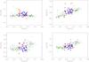 |
Fig. 7 Same as Fig. 6 but for the Fe-peak elements Cr, Mn, Co, and Ni. |
| In the text | |
|
Fig. 8 Δ[X/H] differential abundances (for the α-elements Mg, Si, Ca, and Ti vs. Teff). Dashed-dotted lines represent 1-rms over and below the median for our sample, whereas dotted lines represent the 1.5-rms level. Dashed lines represent the mean differential abundance. Red diamonds are stars compatible within 1-rms with the Fe abundance but not for all elements, blue squares are the candidates selected to become members of the Hyades Supercluster, while green triangles are rejected candidates and starred points are the giants. Blue squares and starred points are the final selected candidates to become members of the Hyades Supercluster. BZ Cet, V683 Per, and ϵ Tau are indicated by orange circles. |
| In the text | |
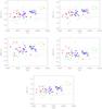 |
Fig. 9 Same as Fig. 8 but for the Fe-peak elements Cr, Mn, Co, and Ni. |
| In the text | |
|
Fig. 10 Comparison of the stellar parameters determined with the Sousa et al. (2008) Fe i-Fe ii line list versus the list from Hekker & Meléndez (2007). |
| In the text | |
|
Fig. 11 Comparison of [X/Fe] derived with the stellar paramaters determined with the Sousa et al. (2008) Fe i-Fe ii line list versus the list from Hekker & Meléndez (2007). Dashed line represents the mean value for the differences. Dashed-dotted lines represent one standard deviation over the mean value. |
| In the text | |
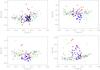 |
Fig. A.1 Same as Fig. 6 but for the odd-Z elements Na, Al, Sc, and V. |
| In the text | |
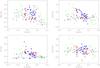 |
Fig. A.2 Same as Fig. 6 but for the s-process elements Ba, Ce, Y, and Zr. |
| In the text | |
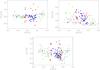 |
Fig. A.3 Same as Fig. 6 but for the s-process elements Cu, Nd, and Zn. |
| In the text | |
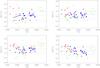 |
Fig. A.4 Same as Fig. 8 but for the odd-Z elements Na, Al, Sc, and V. |
| In the text | |
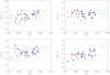 |
Fig. A.5 Same as Fig. 8 but for the s-process elements Ba, Ce, Y, and Zr. |
| In the text | |
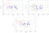 |
Fig. A.6 Same as Fig. 8 but for the s-process elements Cu, Nd, and Zn. |
| In the text | |
Current usage metrics show cumulative count of Article Views (full-text article views including HTML views, PDF and ePub downloads, according to the available data) and Abstracts Views on Vision4Press platform.
Data correspond to usage on the plateform after 2015. The current usage metrics is available 48-96 hours after online publication and is updated daily on week days.
Initial download of the metrics may take a while.