| Issue |
A&A
Volume 547, November 2012
|
|
|---|---|---|
| Article Number | A45 | |
| Number of page(s) | 6 | |
| Section | Stellar structure and evolution | |
| DOI | https://doi.org/10.1051/0004-6361/201117393 | |
| Published online | 24 October 2012 | |
Measuring the orbital inclination of Z Andromedae from Rayleigh scattering
Astronomical Institute, Slovak Academy of Sciences,
059 60
Tatranská Lomnica,
Slovakia
e-mail: This email address is being protected from spambots. You need JavaScript enabled to view it.
Received: 2 June 2011
Accepted: 10 September 2012
Abstract
Context. The orbital inclination of the symbiotic prototype Z And has not been established yet. At present, two very different values are considered, i ~ 44° and i ≳ 73°. The correct value of i is a key parameter in, for example, modeling the highly-collimated jets of Z And.
Aims. To measure the orbital inclination of Z And.
Methods. First, we derive the hydrogen column density (nH), which causes the Rayleigh scattering of the far-UV spectrum at the orbital phase φ = 0.961 ± 0.018. Second, we calculate nH as a function of i and φ for the ionization structure during the quiescent phase. Third, we compare the nH(i,φ) models with the observed value.
Results. The most probable shaping of the H i/H ii boundaries and the uncertainties in the orbital phase limit i of Z And to 59°−2°/+3°. Systematic errors given by using different wind velocity laws can increase i up to ~74°. A high value of i is supported independently by the orbitally related variation in the far-UV continuum and the obscuration of the O i] λ1641 Å emission line around the inferior conjunction of the giant.
Conclusions. The derived value of the inclination of the Z And orbital plane allows treating satellite components of Hα and Hβ emission lines as highly-collimated jets.
Key words: binaries: symbiotic / scattering / stars: individual: Z And
© ESO, 2012
1. Introduction
Symbiotic stars are long-period interacting binaries comprising a cool giant as the donor star and a compact star, most often a white dwarf (WD), as the accretor. This composition requires large orbital periods, which are typically of a few years.
The circumstellar environment of symbiotic stars, which consists of energetic photons from the hot star and neutral particles from the cool giant, represents an ideal medium for the effects of Rayleigh and Raman scattering on neutral hydrogen atoms (e.g., Nussbaumer et al. 1989). The Rayleigh scattering produces a strong attenuation of the continuum around the Ly-α line in systems with a high orbital inclination at positions with the giant in front during quiescent phases (Isliker et al. 1989). The strength of this attenuation is thus determined by nH between the hot star and the observer. Its quantity is a function of the binary position and the orbital inclination, depending on the ionization structure of the binary. For the steady state situation and the quiescent phase, the H i/H ii boundaries were first described by Seaquist et al. (1984; hereafter STB). In the model, the neutral zone is located symmetrically around the binary axis and is usually cone-shaped with the giant at its top facing the ionizing source (e.g., Fig. 7 of Fernández-Castro et al. 1988).
Z And is the prototype of the symbiotic stars class. The binary consists of a late-type, M4.5 III giant and a WD accreting from the giant’s wind on the 759-day orbit (e.g., Nussbaumer & Vogel 1989; Fekel et al. 2000b). Z And was considered to be a non-eclipsing binary. Based on optical observations, Mikołajewska & Kenyon (1996) suggested the orbital inclination i ≈ 50°−70°. Based on polarimetric measurements of the Raman scattered λ6830 line, Schmid & Schild (1997a) and Isogai et al. (2010) determined that i = 47° ± 12° and 41° ± 8°, respectively. On the other hand, a high orbital inclination was supported by (i) the eclipse-like effect measured in the light curve at the position of the inferior conjunction of the giant, which suggested i > 76° (Skopal 2003), (ii) the polarimetric measurements in the continuum, whose modulation along the orbit corresponds to i = 73° ± 14° (Isogai et al. 2010), (iii) the two-temperature type of the ultraviolet (UV) spectrum that develops during active phases of systems with a high orbital inclination (Skopal 2005), and (iv) the presence of the Rayleigh attenuated far-UV continuum measured around the inferior conjunction of the giant during the quiescent phase (e.g. Skopal 2003).
Knowledge of the correct value of i is a key parameter in, for example, modeling the enhanced bipolar mass outflow, launched recently by Z And (Skopal & Pribulla 2006). If i < 55°, this outflow can be treated as a radiatively accelerated wind (Tomov et al. 2010; Kilpio et al. 2011). Otherwise, this type of mass outflow represents highly collimated jets (e.g., Skopal et al. 2009).
In this paper, we model the effect of the Rayleigh scattering measured in the spectrum of Z And from the quiescent phase to derive i. In Sect. 2, we introduce observations and derive the nH parameter, which causes the attenuation effect. In Sect. 3, we introduce the ionization structure of the binary and calculate nH as a function of the orbital phase and the inclination. In Sect. 4, we compare the nH(i,φ) models with the measured value and in this way derive the range of i from Rayleigh scattering. The conclusions are found in Sect. 5.
2. Observations
There are two pairs of UV spectra of Z And in the International Ultraviolet Explorer (IUE) archive taken close to the position of the inferior conjunction of the giant during the quiescent phase: SWP07410 + LWR06393, from December 15th 1979, and SWP32845 + LWP12624, from February 3rd 1988. Both spectra display signatures of the Rayleigh scattering attenuation in the continuum around the Ly-α line. However, the former has underexposed the far-UV continuum and is affected by a strong geocoronal Ly-α emission. Therefore, we treated only the latter spectrum. According to the orbital elements of Fekel et al. (2000b), the spectrum was obtained at the orbital phase φ = 0.961 ± 0.018. Its spectral energy distribution (SED) in the continuum was modeled in the same way as by Skopal (2005). Here, we simplified the model by using only one nebula and adopting zero He++ abundance (Fig. 1). The strong depression of the continuum around Ly-α is caused by the Rayleigh scattering of the continuum photons on the neutral atoms of hydrogen (e.g., Isliker et al. 1989; Vogel 1991; Dumm et al. 1999). In our case, the depression corresponds to nH = (3.9 ± 0.5) × 1022 cm-2.
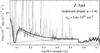 |
Fig. 1 UV observations of Z And carried out close to the inferior conjunction of the giant during its quiescent phase (on February 3rd 1988). Compared is the model SED (heavy solid line) with its components from the nebula (dashed line) and the hot star (thin solid line). The strong attenuation of the continuum around the Ly-α line is caused by the Rayleigh scattering process. Dotted line represents the non-attenuated light (see text for details). |
Having the quantity of nH from observations at the given orbital phase, we can calculate its dependence on the orbital inclination, i, for the ionization structure during the quiescent phase. We introduce the model in the following section.
3. The model
Here, we determine the ionization structure of a symbiotic binary and calculate the column density of neutral hydrogen on the line of sight as a function of φ and i. Comparing theoretical values of nH(i,φ) with those derived independently from observations allows us to estimate the inclination of the orbital plane.
3.1. nH as a function of the orbital inclination
Assuming that the wind from the red giant is spherically symmetric and neutral, the continuity equation determines the particle concentration of hydrogen as 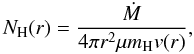 (1)where Ṁ is the mass-loss rate from the giant, r is the distance from its center, μ the mean molecular weight, mH the mass of the hydrogen atom, and v(r) velocity of the wind. Accordingly, we obtain the hydrogen column density, nH, by integrating Eq. (1)along the line of sight, l, from the observer (− ∞) to the ionization boundary as
 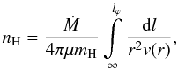 (2)where lϕ is a segment of the line of sight calculated from the intersection of its normal, which connects the giant’s center, to the boundary (Fig. 2). To determine nH we need to know the radius-vector r at each point of the line of sight, which is a function of i and the phase angle, ϕ (ϕ = 0 at the giant’s inferior conjunction). Furthermore, we introduce a parameter b as
 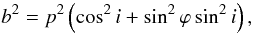 (3)which represents projection of the separation p between the binary components into the plane perpendicular to the line of sight (Fig. 2). Equation (2)may now be expressed as
 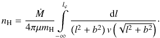 (4)Then, knowing the value of lϕ for a given direction to the ionizing source and the velocity v(r), we can solve Eq. (4)for nH. Figure 2 shows that
 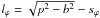 , where sϕ is the distance from the hot star to the H I/H II boundary on the line of sight. Its value is given by the ionization structure during the quiescent phase (Sect. 3.3), which requires knowledge of the velocity v(r) of the giant’s wind, which we introduce below.
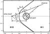 |
Fig. 2 A scheme of a symbiotic binary to calculate nH along the line of sight, l, throughout the neutral H i region (Eq. (4)). The thick solid line represents the H i/H ii boundary (Sect. 3.3) and ϑ is the angle between l and the binary axis. Other auxiliary parameters are introduced in Sect. 3.1. Distances are in units of the binary components separation, p. |
3.2. Velocity profile of the wind from the giant
Vogel (1991) recognized that the column densities nH that he measured from the spectra of EG And cannot be explained by a standard β-law wind (see, e.g., his Eq. (6)). The observed rapid increase of nH values prior to the total eclipse requires a lower velocity in the vicinity of the cool giant (r ≈ Rg) and a much steeper velocity profile for 0.09 ≳ φ ≲ 0.14 (r ≈ 3 Rg with respect to that given by the β-law wind (see Figs. 4 and 7 of Vogel 1991). Therefore, Vogel (1991) employed Eq. (4) to reconstruct a more appropriate velocity field of the wind from cool giants.
Having many more observations covering the eclipse profile of SY Mus due to the Rayleigh scattering, Pereira et al. (1999) and Dumm et al. (1999) solved Eq. (4) for the velocity law v(r) by expanding the function nH(b) into a Taylor series. To match the nH values measured around the eclipse, both groups of authors confirmed independently the claim of a significantly faster acceleration of the wind particles from the giant in comparison with the β-law.
Re-analyzing the wind acceleration zone for the giant in EG And by using a series of FUSE and HST/STIS observations, Crowley et al. (2005) recently confirmed that the wind acceleration region extends only to ~2.5 Rg from the limb of the giant. The corresponding wind velocity profile was very similar to that derived by Dumm et al. (1999) for SY Mus (see their Fig. 7). Therefore, for the purpose of this paper, we use the wind velocity law as derived by Dumm et al. (1999). We note that cool giants in both SY Mus and Z And have the same spectral type (M 4.5, Mürset & Schmid 1999) and similar other fundamental parameters (see Table 2 of Skopal 2005), which also supports adoption of the wind law (7) for the case of Z And.
According to Dumm et al. (1999), it was sufficient to approximate the nH(b) function by two terms of the Taylor expansion (k = 1 and k ≈ 20), which allows expressing the velocity law in a form 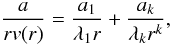 (5)where a = 2Ṁ/4πμmHv∞Rg, a1, ak and k are parameters, and λk is defined recursively as
 ![Mathematical equation: \begin{equation} \lambda_1 = \pi/2, \hskip 1cm \lambda_k= \pi/\left[\left(2k-2\right)\lambda_{k-1}\right]. \label{lambda} \end{equation}](/articles/aa/full_html/2012/11/aa17393-11/aa17393-11-eq58.png) (6)Fitting the observed nH as a function of the impact parameter b, Dumm et al. (1999) derived a1 ≈ 4.5 × 1023 cm-2, a ≈ 3 × 1023 cm-2, k ≈ 20 and a20 ≈ 1 × 1031 cm-2. Using these values we can rewrite Eq. (5)in the form
(6)Fitting the observed nH as a function of the impact parameter b, Dumm et al. (1999) derived a1 ≈ 4.5 × 1023 cm-2, a ≈ 3 × 1023 cm-2, k ≈ 20 and a20 ≈ 1 × 1031 cm-2. Using these values we can rewrite Eq. (5)in the form  (7)where r is the distance from the center of the giant in units of its radius. According to this law, the main acceleration zone of the wind is located between the giant’s photosphere and r = 3 (v(3)/v∞ ~ 0.9, λ20 = 0.2838).
 |
Fig. 3 H i/H ii boundaries in a symbiotic binary given by solution of Eq. (9)for the velocity law (7)of the giant wind. This represents basic ionization structure of the circumstellar matter in symbiotic binaries during quiescent phases as originally outlined by STB (Sect. 1). |
3.3. Ionization structure
The distance sϕ from the ionization boundary to the WD (Fig. 2) is determined by a balance between the ionizing photons emitted in a small angle around the direction ϑ and recombinations in this angle. According to Nussbaumer & Vogel (1987), the equilibrium condition can be expressed as  (8)where Lph is the number of photons capable of ionizing hydrogen that are emitted spherically-symmetrically from the hot star per second, s is the distance from the hot star, NH+ and Ne are concentrations of protons and electrons, respectively, and αB is the total hydrogen recombination coefficient for recombinations other than to the ground state. In the H+ region, we consider that Ne = NH = NH+. Then, assuming that Te is constant throughout the nebula and thus also αB, condition (8)can be expressed as
  (9)where XH+ is the ionization parameter (STB),
 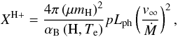 (10)and
 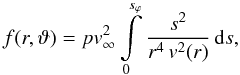 (11)where we used the particle concentration in the giant’s wind as given by Eq. (1), and
 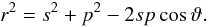 (12)Examples of H i/H ii boundaries are depicted in Fig. 3.
4. Orbital inclination of Z And
Having defined ionization structure, we can solve Eq. (9)for sϕ, which determines lϕ and thus nH (see Fig. 2, Eq. (4)) for the ionization parameter XH+. Its value is given by the binary parameters. Therefore, first we find a possible range of XH+.
For Porb = 759 days (Fekel et al. 2000b) and the total mass of the binary, 2.6 M⊙ (Mikołajewska & Kenyon 1996), we get the separation of the stars, p = 480 R⊙. Furthermore, we adopt αB(H,Te) = 1.43 × 10⁻¹³ cm3 s-1 for Te = 20 000 K (Nussbaumer & Vogel 1987) and Ṁ ~ 7 × 10⁻⁷ M⊙ yr-1, derived from the total emission measure during quiescence (Skopal 2005). This value of Ṁ represents an upper limit because of the presence of other sources of the nebular radiation, e.g., the hot star wind. The hot star luminosity Lh ~ 2300(d/1.5 kpc)2 L⊙ and a temperature of ~120 000 K (Table 3 of Skopal 2005) yield Lph ~ 1.5 × 1047(d/1.5 kpc)2 s-1. Assuming a typical value for the terminal velocity for the giant wind, v∞ ≈ 40 km s-1 (Reimers 1981), we obtain XH+ ≈ 20. We note that Fernández-Castro et al. (1988) derived XH+ ≈ 14. However, there are more sources of uncertainties in determining the parameter XH+: (i) terminal velocity for the massive slow wind from the giant was also assumed to be of 20 km s-1 only (e.g., Dumm et al. 1999). This value scales the above derived XH+ with a factor of 0.25; (ii) a smaller distance to Z And of 1.12 kpc and 1.2 kpc (Fernández-Castro et al. 1988; Sokoloski et al. 2006) reduces the luminosity and thus the value of XH+ with a factor of 0.55 and 0.64, respectively; (iii) a maximum Zanstra temperature of 130 000 K (Mürset et al. 1991) gives Lh = 3400(d/1.5 kpc)2 L⊙, i.e. Lph = 2.2 × 1047(d/1.5 kpc)2 s-1, which enlarges the above value of XH+ = 20 with a factor of ~1.5. According to these possibilities we consider a range of the ionization parameter as 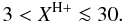 (13)In the following subsection, we explore the nH(i,φ) function at the position of φ = 0.961 ± 0.018, when the IUE observations were exposed.
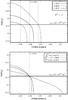 |
Fig. 4 Top: calculated column densities (Eq. (4)) as a function of the orbital phase for the H i zone defined by the mean value of XH+ = 17 (relations (10) and (13)). Particle concentration along the line of sight (Eq. (1)) was calculated for v∞ = 40 km s-1. Solutions giving nH = 3.9 × 1022 cm-2 at the orbital phases φ = 0.961 ± 0.018 (dotted lines) are plotted. Bottom: as in the top, but for 3 ≲ XH+ ≲ 30 and φ = 0.961. |
4.1. Modeling the column density at φ = 0.961
The top panel of Fig. 4 shows the resulting column densities as a function of the orbital phase, calculated for the average value of XH+ = 17, for which nH(i,φ = 0.961 ± 0.018) = 3.9 × 1022 cm-2. The range of possible orbital phases limits the inclination angle to i = 59°−2°/+3°. In the bottom panel of Fig. 4, the nH(i,φ) function was calculated for the range of possible XH+ (Eq. (13)). Here, the models for different values of XH+, satisfying nH(i,0.961) = 3.9 × 1022 cm-2, restrict the orbital inclination to i = 59°−2°/+1°. Small uncertainties reflect small differences between opening angles of H i zones for larger values of XH+ (see Fig. 3). Figure 5 illustrates the calculated nH(i,0.961) as a function of i for the range of the parameter XH+. From the figure, we can see that the uncertainty in the measured value of nH can enlarge the resulting uncertainty in i by a few degrees. However, systematic errors can result from using a different wind velocity law. Although the used v(r) satisfies best the measured nH as a function of the parameter b (Sect. 3.2), its high values ≳1024 cm-2 in the vicinity of the stellar disk of the giant cannot be measured accurately (see Fig. 5 of Dumm et al. 1999). This precludes a correct determination of the wind law. The nH(b) values, as measured prior to and after the inferior conjunction of the giant, also reflect an asymmetry of the neutral wind zone with respect to the binary axis (see Fig. 4 of Dumm et al. 1999). The used wind law (7) was derived from the egress data. Thus, the steeper ingress data will correspond to a steeper v(r). Therefore, we also investigated a limiting case for a maximum steepness of v(r) = v∞. This approach yielded  /
/ . From this point of view, the orbital inclination of Z And can be expected to be in the range of ~59°−74°.
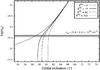 |
Fig. 5 As in the bottom panel of Fig. 4, but for nH(i,φ = 0.961) as a function of i. Solution for XH+ = 100 was added to demonstrate the small change of i for very high XH+ (Sect. 4.1). Intersections of the model curves with the horizontal line at the observed value of nH = 3.9 × 1022 cm-2 correspond to i = 57, 59, 59.5, and 60 |
Finally, the dependence of i on Ṁ follows that on XH+, because XH+ ∝ Ṁ-2 (Eq. (10)). This implies that Ṁ < upper limit of 7 × 10⁻⁷ M⊙ yr-1 (see above) yields higher XH+, which, however, has no significant effect on the corresponding value of i, because the opening angle of the neutral zone, ϑ∞, decreases very slowly for XH+ > 10 (see Fig. 3). For example, the lower value of Ṁ = 3.1 × 10⁻⁷(d/1.5 kpc)3/2 M⊙ yr-1, derived by Fernández-Castro et al. (1988) from radio observations, enlarges the range of XH+ (13) by a factor of ~5, i.e. 15 < XH+ ≲ 150. Figure 5 also shows the model nH(i,0.961) for XH+ = 100, which demonstrates only a small increase of i to 60 7.
7.
4.2. The far-UV light curve
The high orbital inclination of Z And is also supported by a large variation in the far-UV continuum along the orbit as measured on IUE spectra. Figure 6 shows examples of fluxes measured around λ1280 Å, which is relatively free of emission/absorption features. Similar variations are indicated also at longer wavelengths, where the influence of the Rayleigh scattering is negligible. For example, we selected fluxes at ~λ1600 Å, where instead the iron curtain absorption could be pronounced (see Shore & Aufdenberg 1993). The variation here has a smaller amplitude with a shallow minimum with respect to that at ~λ1280 Å. Generally, the UV continuum peaks around the superior conjunction of the giant, while at the opposite site the fluxes are significantly fainter. This variability reflects the presence of an additional source of extinction, which attenuates more the short wavelength part of the UV spectra. This effect is known for eclipsing symbiotic binaries RW Hya, SY Mus, and EG And (Dumm et al. 1999; Crowley et al. 2008). The influence of the absorbing medium was modeled by Horne et al. (1994), who found that the absorbing gas produces a modest optical depth in the Balmer and Pashen continuum, which can make it significantly lower in the UV (see their Fig. 8). As the absorbing material is concentrated more on the orbital plane and enhanced at positions with the giant in front, the large amplitude of the far-UV continuum can be attributed to a high orbital inclination of Z And. In contrast, the non-eclipsing symbiotic binary AG Dra (i ≈ 30−45° or i ~ 60°, Mikołajewska et al. 1995; Schmid & Schild 1997b) does not show such variability in the UV spectrum (Fig. 6).
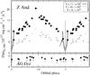 |
Fig. 6 Variation in the far-UV, 1280 Å (•) and 1600 Å (+ ) fluxes of Z And and AG Dra along their orbits as measured on the IUE spectra during their quiescent phases. The arrow points the flux from the spectrum in Fig. 1. The lines around φ = 0 and 1 represent Rayleigh attenuated light curves for models in keys. Orbital elements of Fekel et al. (2000b) were used. |
Finally, we calculated the Rayleigh scattered light curves for the nH(i,φ) functions depicted in the bottom panel of Fig. 4, scaled to the observed flux at φ = 0.961 (see Fig. 6). The aim here is to model the expected Rayleigh attenuation as a function of φ and to check how it is connected with the neighboring measurements. Assuming that the Rayleigh scattering is the only process attenuating the far-UV continuum, we can write the observed flux as 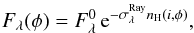 (14)where
  is the original flux and
  is the Rayleigh scattering cross section. For F1280(0.961) = 6.5 × 10⁻¹³ erg cm-2 s-1 Å-1 (Fig. 6), nH(0.961) = 3.9 × 1022 cm-2 (Fig. 1) and
  cm2 (Nussbaumer et al. 1989) we get the unscattered flux
  erg cm-2 s-1 Å-1. Then, according to Eq. (14), we calculated the light curve F1280(φ) for the three models nH(i,φ) plotted in Fig. 4. The result is shown in Fig. 6. The rather narrow (≲ 0.1 Porb) and deep model light curves reflect a close cut of the H i region for the resulting inclinations and the strong dependence of the Rayleigh attenuation on nH. In other words, due to a small opening angle of the neutral zone (ϑ∞ ~ 35° and 34° for X = 17 and X = 30, respectively), their cut with the line connecting the hot star and the observer along the orbit covers only a small segment of the orbital period. Overall, the Rayleigh scattering light curves, calculated according to our resulting nH(i,φ) models, seem to be consistent with the fluxes measured around the inferior conjunction of the giant.
4.3. A probe of a high inclination with the O I] 1641 Å line
Shore & Wahlgren (2010) investigated observational properties of the intercombination transition O i] 1641 Å to a metastable state in the spectra of some symbiotic stars with the aim of diagnosing the neutral red giant wind. Their idea is based on the following: (i) the ionization potential of both oxygen and hydrogen is comparable, (ii) the oxygen resonance multiplet (1302, 1304, 1305 Å) is, in addition to the ground state, connected to two metastable states through emission at 1641 Å and 2324 Å (see Fig. 1 of Shore & Wahlgren 2010), and (iii) the intercombination transition at λ1641 Å can be stimulated by absorption from the ground state of the O i 1302 Å resonance line in the surrounding neutral gas. This implies that the O i 1302 Å emission line, which is formed by recombinations within the extended H ii region, surrounds closely the neutral H i region during quiescent phases of symbiotic stars and thus gives rise to the measurable O i] 1641 Å emission within the neutral wind from the cool giant. Shore & Wahlgren (2010) found that the O i] variations are strongly correlated with the optical light curves and also with the O vi Raman emission at λ6825, 7082 Å. Both the O i] 1641 Å and the Raman lines are optically thin; the transitions are not repeatable: once they happen, their photons escape the medium. As a result, the transitions arise in the red giant wind close to the H i/H ii interface, preferentially between the binary components with the highest density of the giant’s wind (in contrast to the Rayleigh scattering, which is a repeatable process and thus measures the total thickness of the neutral wind). Shore & Wahlgren (2010) confirmed this view for the eclipsing system EG And, where the O i] line was obscured around the inferior conjunctions of the giant. For low-inclination systems, the authors suggested that these lines should always be visible.
Accordingly, to probe the orbital inclination of Z And, we plotted the O i] 1641 Å line fluxes of Z And from its quiescent phase together with those of the eclipsing symbiotic binary EG And in the phase diagram (Fig. 7). The figure demonstrates that around the inferior conjunction of the giant (φ = 0 or 1), the O i] fluxes are very weak (EG And) or not measurable (Z And). Maximum values were measured when the line of sight does not intersect the neutral hydrogen zone (the light gray belts in Fig. 7). For EG And, the extent of the H i region in the phase diagram (Δφ = ± 0.16) was determined for i = 90° (Vogel et al. 1992) and the position of the H i/H ii boundary at b ≈ 3.5 Rg (see Fig. 7 of Crowley et al. 2005, and Eq. (3) here). In the case of Z And, the range of intersections of the line of sight with the neutral zone in the phase diagram (Δφ = ± 0.11, 0.048, 0.044; dotted lines in Fig. 7) corresponds to our models for X = 3, 17, 30 from the bottom panel of Fig. 4. The results are consistent with the properties and the formation region of the O i] 1641 Å line during quiescent phases, as described above. Thus, the occultation of the O i] fluxes of Z And during its quiescent phase independently supports a higher inclination of its orbit.
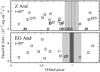 |
Fig. 7 Variations of the O i] 1641 Å line fluxes during quiescent phases of Z And and EG And as a function of the orbital phase according to the ephemeris of Fekel et al. (2000a) and Fekel et al. (2000b), respectively. The light gray belts correspond to the intersection of the H i zone with the line of sight along the orbit (see Sect. 4.3). The dark belt reflects a time interval of the total eclipse of the point source by the giant in EG And (Δφ = ± 0.038; see Table 1 of Crowley et al. 2008). Fluxes were taken from Figs. 4 and 8 of Shore & Wahlgren (2010). |
5. Conclusion
We used IUE observations of the symbiotic star Z And, which were taken during its quiescent phase around the inferior conjunction of the giant, to determine the inclination of its orbital plane.
First, we derived nH = 3.9 ± 0.5 × 1022 cm-2 (Fig. 1) on the line of sight, which passes throughout the neutral zone of the giant’s wind toward the hot star at the time of the observation (at φ = 0.961 ± 0.018), by modeling the Rayleigh scattering of the far-UV continuum (Sect. 2). Second, we determined the STB ionization structure for the velocity profile of the giant’s wind as derived by Dumm et al. (1999, Fig. 3), and calculated nH(i,φ) as a function of the orbital inclination and the phase (Figs. 4 and 5). Third, comparing the nH(i,φ) function with the observed value of 3.9 × 1022 cm-2, we estimated the range of orbital inclinations as follows: (i) for the average value of the parameter XH+ = 17, i = 59°−2°/ +3°, where the uncertainties reflect those in the binary position, and (ii) for the most probable position of the binary at φ = 0.961, the range of 3 ≲ XH+ ≲ 30 restricts the orbital inclination to i = 59°−2°/ +1°. Systematic errors given
by using different wind velocity laws can increase i up to ~74° (Sect. 4.1). Fluxes, that are measured around the inferior conjunction of the giant are consistent with the Rayleigh scattering light curves (Eq. (14)) calculated for our resulting nH(i,φ) models (Fig. 6).
The high value of the orbital inclination is also supported by the large amplitude of the orbitally related variation in the far-UV continuum (Sect. 4.2, Fig. 6) and by the obscuration of the O i] 1641 Å fluxes around the inferior conjunctions of the giant during the quiescent phase of Z And (Sect. 4.3, Fig. 7).
Finally, the higher value of the inclination of the Z And orbital plane allows us to interpret the satellite components of Hα and Hβ emission lines, which appeared during active phases from 2006 as highly collimated jets rather than as a special type of radiatively accelerated wind.
Acknowledgments
We thank the anonymous referee for constructive comments. This research was supported by a grant of the Slovak Academy of Sciences, VEGA No. 2/0038/10. This article was also supported by the realization of the Project ITMS No. 26220120029, based on the supporting operational Research and development program financed from the European Regional Development Fund.
References
- Crowley, C., Espey, B. R., & McCandliss, S. R. 2005, in Proc. 13th Cambridge Workshop on Cool Stars, Stellar Systems and the Sun, eds. F. Favata, G. Hussain, & B. Battrick, ESA SP, 560, 343 [Google Scholar]
- Crowley, C., Espey, B. R., & McCandliss, S. R. 2008, ApJ, 675, 711 [NASA ADS] [CrossRef] [Google Scholar]
- Dumm, T., Schmutz, W., Schild, H., & Nussbaumer, H. 1999, A&A, 349, 169 [NASA ADS] [Google Scholar]
- Fekel, F. C., Joyce, R. R., Hinkle, K. H., & Skrutskie, M. 2000a, AJ, 119, 1375 [NASA ADS] [CrossRef] [Google Scholar]
- Fekel, F. C., Hinkle, K. H., Joyce, R. R., & Skrutskie, M. 2000b, AJ, 120, 3255 [NASA ADS] [CrossRef] [Google Scholar]
- Fernández-Castro, T., Cassatella, A., Giménez, A., & Viotti, R. 1988, ApJ, 324, 1016 [NASA ADS] [CrossRef] [Google Scholar]
- Horne, K., Marsh, T. R., Cheng, F. H., Hubený, I., & Lanz, T. 1994, ApJ, 426, 294 [NASA ADS] [CrossRef] [Google Scholar]
- Isliker, H., Nussbaumer, H., & Vogel, M. 1989, A&A, 219, 271 [NASA ADS] [Google Scholar]
- Isogai, M., Seki, M., Ykeda, Y., Akitaya, H., & Kawabata, K.S. 2010, AJ, 140, 235 [NASA ADS] [CrossRef] [Google Scholar]
- Kilpio, E., Bisikalo, D., Tomov, N., & Tomova, M. 2011, Ap&SS, 335, 155 [NASA ADS] [CrossRef] [Google Scholar]
- Mikołajewska, J., & Kenyon, S. J. 1996, AJ, 112, 1659 [NASA ADS] [CrossRef] [Google Scholar]
- Mikołajewska, J., Kenyon, S. J., Mikołajewski, M., Garcia, M. R., & Polidan, R. S. 1995, AJ, 109, 1289 [NASA ADS] [CrossRef] [Google Scholar]
- Mürset, U., & Schmid, H. M. 1999, A&AS, 137, 473 [NASA ADS] [CrossRef] [EDP Sciences] [Google Scholar]
- Mürset, U., Nussbaumer, H., Schmid, H. M., & Vogel, M. 1991, A&A, 248, 458 [NASA ADS] [Google Scholar]
- Nussbaumer, H., & Vogel, M. 1987, A&A, 182, 51 [NASA ADS] [Google Scholar]
- Nussbaumer, H., & Vogel, M. 1989, A&A, 213, 137 [NASA ADS] [Google Scholar]
- Nussbaumer, H., Schmid, H. M., & Vogel, M. 1989, A&A, 211, L27 [NASA ADS] [Google Scholar]
- Pereira, C. B., Ortega, V. G., & Monte-Lima, I. 1999, A&A, 344, 607 [NASA ADS] [Google Scholar]
- Reimers, D. 1981, in Physical Processes in Red Giants, eds. I. Iben, & A. Renzini (Dordrecht: Reidel), 269 [Google Scholar]
- Schmid, H. M., & Schild, H. 1997a, A&A, 327, 219 [NASA ADS] [Google Scholar]
- Schmid, H. M., & Schild, H. 1997b, A&A, 321, 791 [NASA ADS] [Google Scholar]
- Seaquist, E. R., Taylor, A. R., & Button, S. 1984, ApJ, 284, 202 (STB) [NASA ADS] [CrossRef] [Google Scholar]
- Shore, S. N., & Aufdenberg, J. P. 1993, ApJ, 416, 355 [NASA ADS] [CrossRef] [Google Scholar]
- Shore, S. N., & Wahlgren, G. M. 2010, A&A, 515, A108 [NASA ADS] [CrossRef] [EDP Sciences] [Google Scholar]
- Skopal, A. 2003, A&A, 401, L17 [NASA ADS] [CrossRef] [EDP Sciences] [Google Scholar]
- Skopal, A. 2005, A&A 440, 995 [NASA ADS] [CrossRef] [EDP Sciences] [Google Scholar]
- Skopal, A., & Pribulla, T. 2006, ATel. No. 882 [Google Scholar]
- Skopal, A., Pribulla, T., Budaj, J., et al. 2009, ApJ, 690, 1222 [NASA ADS] [CrossRef] [Google Scholar]
- Sokoloski, J. L., Kenyon, S. J., Espey, B. R., et al. 2006, ApJ, 636, 1002 [NASA ADS] [CrossRef] [Google Scholar]
- Tomov, N. A., Bisikalo, D. V., Tomova, M. T., & Kil’pio, E. Yu. 2010, Astron. Rep., 54, 628 [NASA ADS] [CrossRef] [Google Scholar]
- Vogel, M. 1991, A&A, 249, 173 [NASA ADS] [Google Scholar]
- Vogel, M., Nussbaumer, H., & Monier, R. 1992, A&A, 260, 156 [NASA ADS] [Google Scholar]
All Figures
|
Fig. 1 UV observations of Z And carried out close to the inferior conjunction of the giant during its quiescent phase (on February 3rd 1988). Compared is the model SED (heavy solid line) with its components from the nebula (dashed line) and the hot star (thin solid line). The strong attenuation of the continuum around the Ly-α line is caused by the Rayleigh scattering process. Dotted line represents the non-attenuated light (see text for details). |
| In the text | |
|
Fig. 2 A scheme of a symbiotic binary to calculate nH along the line of sight, l, throughout the neutral H i region (Eq. (4)). The thick solid line represents the H i/H ii boundary (Sect. 3.3) and ϑ is the angle between l and the binary axis. Other auxiliary parameters are introduced in Sect. 3.1. Distances are in units of the binary components separation, p. |
| In the text | |
|
Fig. 3 H i/H ii boundaries in a symbiotic binary given by solution of Eq. (9)for the velocity law (7)of the giant wind. This represents basic ionization structure of the circumstellar matter in symbiotic binaries during quiescent phases as originally outlined by STB (Sect. 1). |
| In the text | |
|
Fig. 4 Top: calculated column densities (Eq. (4)) as a function of the orbital phase for the H i zone defined by the mean value of XH+ = 17 (relations (10) and (13)). Particle concentration along the line of sight (Eq. (1)) was calculated for v∞ = 40 km s-1. Solutions giving nH = 3.9 × 1022 cm-2 at the orbital phases φ = 0.961 ± 0.018 (dotted lines) are plotted. Bottom: as in the top, but for 3 ≲ XH+ ≲ 30 and φ = 0.961. |
| In the text | |
|
Fig. 5 As in the bottom panel of Fig. 4, but for nH(i,φ = 0.961) as a function of i. Solution for XH+ = 100 was added to demonstrate the small change of i for very high XH+ (Sect. 4.1). Intersections of the model curves with the horizontal line at the observed value of nH = 3.9 × 1022 cm-2 correspond to i = 57, 59, 59.5, and 60 |
| In the text | |
|
Fig. 6 Variation in the far-UV, 1280 Å (•) and 1600 Å (+ ) fluxes of Z And and AG Dra along their orbits as measured on the IUE spectra during their quiescent phases. The arrow points the flux from the spectrum in Fig. 1. The lines around φ = 0 and 1 represent Rayleigh attenuated light curves for models in keys. Orbital elements of Fekel et al. (2000b) were used. |
| In the text | |
|
Fig. 7 Variations of the O i] 1641 Å line fluxes during quiescent phases of Z And and EG And as a function of the orbital phase according to the ephemeris of Fekel et al. (2000a) and Fekel et al. (2000b), respectively. The light gray belts correspond to the intersection of the H i zone with the line of sight along the orbit (see Sect. 4.3). The dark belt reflects a time interval of the total eclipse of the point source by the giant in EG And (Δφ = ± 0.038; see Table 1 of Crowley et al. 2008). Fluxes were taken from Figs. 4 and 8 of Shore & Wahlgren (2010). |
| In the text | |
Current usage metrics show cumulative count of Article Views (full-text article views including HTML views, PDF and ePub downloads, according to the available data) and Abstracts Views on Vision4Press platform.
Data correspond to usage on the plateform after 2015. The current usage metrics is available 48-96 hours after online publication and is updated daily on week days.
Initial download of the metrics may take a while.