| Issue |
A&A
Volume 546, October 2012
|
|
|---|---|---|
| Article Number | A73 | |
| Number of page(s) | 20 | |
| Section | Galactic structure, stellar clusters and populations | |
| DOI | https://doi.org/10.1051/0004-6361/201219471 | |
| Published online | 09 October 2012 | |
The VLT-FLAMES Tarantula Survey⋆,⋆⋆
VII. A low velocity dispersion for the young massive cluster R136
1
Scottish Universities Physics Alliance (SUPA), Institute for Astronomy,
University of Edinburgh, Blackford
Hill, Edinburgh
EH9 3HJ, UK
e-mail: vhb@roe.ac.uk
2
UK Astronomy Technology Centre, Royal Observatory
Edinburgh, Blackford
Hill, Edinburgh,
EH9 3HJ,
UK
3
Astronomical Institute “Anton Pannekoek”, University of
Amsterdam, Postbus
94249, 1090 GE,
Amsterdam, The
Netherlands
4
Institute of Astronomy, University of Cambridge,
Madingley Road, Cambridge, CB3 0HA, UK
5
Excellence Cluster Universe, Technische Universität
München, Boltzmannstr.
2, 85748
Garching,
Germany
6
Instituto de Astrofísica de Andalucía-CSIC,
Glorieta de la Astronomía s/n,
18008
Granada,
Spain
7
Institute of Astronomy with NAO, Bulgarian Academy of
Sciences, PO Box
136, 4700
Smoljan,
Bulgaria
8
School of Physics, University of Exeter,
Stocker Road, Exeter
EX4 4QL,
UK
9
European Southern Observatory, Karl-Schwarzschild-Strasse 2, 87548
Garching bei München,
Germany
10
Harvard-Smithsonian CfA, 60 Garden Street, Cambridge, MA
02138,
USA
11 Dept. of Physics & Astronomy,
Hounsfield Road, University of Sheffield, S3 7RH, UK
12
Astrophysics Group, Lennard-Jones Laboratories, Keele
University, Staffordshire
ST5 5BG,
UK
Received:
24
April
2012
Accepted:
3
August
2012
Detailed studies of resolved young massive star clusters are necessary to determine their dynamical state and evaluate the importance of gas expulsion and early cluster evolution. In an effort to gain insight into the dynamical state of the young massive cluster R136 and obtain the first measurement of its velocity dispersion, we analyse multi-epoch spectroscopic data of the inner regions of 30 Doradus in the Large Magellanic Cloud obtained as part of the VLT-FLAMES Tarantula Survey. Following a quantitative assessment of the variability, we use the radial velocities of non-variable sources to place an upper limit of 6 km s-1 on the line-of-sight velocity dispersion of stars within a projected distance of 5 pc from the centre of the cluster. After accounting for the contributions of undetected binaries and measurement errors through Monte Carlo simulations, we conclude that the true velocity dispersion is likely between 4 and 5 km s-1 given a range of standard assumptions about the binary distribution. This result is consistent with what is expected if the cluster is in virial equilibrium, suggesting that gas expulsion has not altered its dynamics. We find that the velocity dispersion would be ~25 km s-1 if binaries were not identified and rejected, confirming the importance of the multi-epoch strategy and the risk of interpreting velocity dispersion measurements of unresolved extragalactic young massive clusters.
Key words: binaries: spectroscopic / galaxies: star clusters: individual R136 / Magellanic Clouds / stars: early-type / stars: kinematics and dynamics
Appendices A and B are available in electronic form at http://www.aanda.org
© ESO, 2012
1. Introduction
The expression “infant mortality” of star clusters was initially coined by Lada & Lada (2003) to describe the discrepancy between the number of observed open clusters and the number of embedded clusters. These authors argued that there are about ten times fewer open clusters than expected if all embedded clusters evolve into open clusters. The rapid removal of gas left-over from star formation was suggested to explain the apparent disruption of such a large fraction of clusters (e.g. Geyer & Burkert 2001; Kroupa & Boily 2002; Bastian & Goodwin 2006). The importance of the infant mortality scenario however depends on the definition adopted for embedded clusters (Bressert et al. 2010; Bastian 2011), with more conservative criteria requiring less than 50% of clusters to be destroyed to match the observed number of open clusters. But no matter which definition is adopted, the question of whether or not gas expulsion plays a significant role in the early evolution/disruption of star clusters still needs to be addressed.
Star clusters have been observed to expand in their first 100 Myr (Mackey & Gilmore 2003; Bastian et al. 2008; Portegies Zwart et al. 2010), but this expansion is not direct evidence for the importance of gas expulsion. There are two ways for clusters to expand as a response to mass loss (e.g. Hills 1980): (i) expansion following impulsive mass loss, e.g. change of potential due to removal of mass faster than the crossing time of the cluster, leaving the cluster in a super-virial state for a few crossing times, or (ii) adiabatic expansion, e.g. driven by stellar evolution on a slow timescale compared to the crossing time of the cluster (~10 Myr for young massive clusters, e.g. Portegies Zwart et al. 2010), in which case the cluster remains in virial equilibrium. Thus, the best way to evaluate the importance of rapid gas expulsion (case i) and the implications for the formation and early evolution of star clusters is to determine the dynamical state of young clusters. In particular, it is important to verify if clusters are in virial equilibrium from a young age.
Attempts to determine the dynamical state of young clusters have been made by comparing dynamical masses (obtained through measuring the velocity dispersion and size of a cluster) and photometric masses (estimated from the age and integrated luminosity). For several unresolved extragalactic star clusters with ages of less than ~10 Myr, the dynamical mass has been found to be up to ten times larger than the photometric mass (e.g. Bastian et al. 2006). This led to the suggestion that these clusters might be super-virial and expanding following gas expulsion (Goodwin & Bastian 2006). However, Gieles et al. (2010b) showed that the increase in the measured line-of-sight velocity dispersion in these young clusters could be produced by the orbital motions of massive binaries. Massive stars indeed dominate the light of young massive clusters and their binary fraction is high (e.g. Mason et al. 2009; Barbá et al. 2010; Sana & Evans 2011; Sana et al. 2012b – hereafter Paper VIII). Therefore, the role of gas expulsion cannot be investigated through observations of unresolved extragalactic clusters.
Detailed dynamical studies of individual resolved clusters (i.e. in the Galaxy, Small Magellanic Cloud – SMC – or Large Magellanic Cloud – LMC) are necessary to make progress. In the case of radial velocity (RV) surveys, multi-epoch observations are needed to detect binaries, which can then be removed and allow a cleaner estimate of the velocity dispersion (unless the orbital solution is known, in which case the centre-of-mass velocity can be included in the dispersion calculation). The young massive cluster R136 (M ~ 105 M⊙, Andersen et al. 2009), in the 30 Doradus region of the LMC, is an ideal target to test the impact of gas expulsion given its young age of less than 2 Myr (de Koter et al. 1998; Massey & Hunter 1998; Crowther et al. 2010).
The identification of binaries was central to the study of stellar dynamics in 30 Doradus with the Gemini Multi-Object Spectrograph by Bosch et al. (2009), who found that the velocity dispersion of NGC 2070 went from ~30 km s-1 to 8.3 km s-1 after correcting for orbital motions, confirming their prediction (Bosch et al. 2001) that the high velocity dispersion of NGC 2070 could be due to undetected binaries. In order to perform a similar study for the dense surroundings of R136, a different observational approach was required because this region is too crowded for fibre spectroscopy. A key component of the VLT-FLAMES Tarantula Survey (VFTS; Evans et al. 2011, hereafter Paper I) is multi-epoch spectroscopy in the inner part of 30 Dor with the FLAMES-ARGUS integral-field unit (IFU), which we use here to obtain an estimate of the velocity dispersion of “single” stars in R136. The central velocity dispersion is an important proxy for the dynamical state of the cluster and is required to estimate, for example, the central potential and relaxation time-scale, both of which are required for detailed numerical (N-body) calculations of R136-like objects (e.g. Portegies Zwart et al. 1999; Gieles et al. 2010a). As a result of the same study, the identification of massive binaries could provide important clues to the star-formation process and the subsequent dynamical evolution of R136, in which binaries can be formed, ejected and destroyed. Our measurements will also serve as useful empirical input for the modelling of stellar interactions in dense clusters, such as the recent studies of Fujii & Portegies Zwart (2011) and Banerjee et al. (2012).
We report here on a velocity dispersion estimate for the young massive cluster R136. We describe the FLAMES-ARGUS IFU data in Sect. 2. In Sect. 3, we present our RV and variability analysis of the stars observed with ARGUS. In Sect. 4, we discuss the spectral classification of the non-variable ARGUS sources. In Sect. 5, we briefly introduce the VFTS Medusa data complementing the ARGUS data. We calculate the velocity dispersion from the stars showing no variability and also estimate the contribution of errors and undetected binaries in Sect. 6. The implications of the measured velocity dispersion for the dynamical state of R136 are discussed in Sect. 7. Finally, we present our conclusions in Sect. 8.
2. ARGUS data
The main data used in this paper consist of five ARGUS IFU pointings in the central arcminute of 30 Dor (see Fig. 2 of Paper I), for which at least five epochs were obtained. This central region is relatively gas free, so the nebular contamination in the spectra is not as important as in other regions of 30 Dor. Spectra of 41 different sources, corrected to the heliocentric frame, were extracted from the data cubes. To probe the stellar dynamics of R136, the LR02 setting of the Giraffe spectrograph was used (λ = 3960–4570 Å, Δλ = 0.40 Å, R ≡ λ/Δλ ~ 10 500). This setting gives access to several stellar absorption lines suitable for RV analysis (see Sect. 3) at the typical signal-to-noise ratio (S/N) of ~85 of our single-epoch spectra. To optimise the detection of binaries, the first two epochs were observed without time restrictions, and the third and fourth were observed with a minimum interval of 28 days between both the second and third, and third and fourth epochs. The fifth epoch was observed at least one year after the first epoch. Some observations were repeated due to changes in conditions and other operational issues, providing additional epochs for three of the five pointings. Note that expanding the time baseline of the observations enhances the chances of detecting long-period binaries, but these binaries are the ones that have a smaller impact on the velocity dispersion enhancement. Further details on the ARGUS data, the reduction and the extraction procedure can be found in Paper I.
For the analysis presented in this paper, individual exposures were considered to belong to the same epoch if their start time was separated by less than one hour. The multiple exposures composing a single epoch were then averaged using the errors (propagated throughout the reduction process) as weights and performing a 5σ clip around the median to remove remaining cosmic features. The spectra from individual exposures had already been normalised as part of the extraction procedure. The resulting epochs, their modified Julian date, and the corresponding ARGUS pointings and exposures are listed in Table A.1.
An effort was made to extract spectra preferably for sources that appeared single by comparing the ARGUS data cubes with an archival HST Wide-Field Camera Three (WFC3) F555W image (De Marchi et al. 2011) and identifying matching sources (see Paper I). Out of 41 ARGUS sources, 23 are dominated by one bright source from the WFC3 image. For these 23 ARGUS sources, only stars at least a factor of ten fainter (in data counts) are visible in the WFC3 image within the region covered by the ARGUS spatial pixels from which the spectrum was extracted. Even if those fainter stars were contaminating the ARGUS spectrum, it is doubtful that they would contribute significantly to the helium absorption lines used for our RV analysis (Sect. 3.2). The ARGUS spatial elements for a further 11 extracted sources are dominated by one bright object from the WFC3 image, but could suffer from more significant contamination from nearby stars (typically at a level of ~20%). The remaining seven ARGUS sources appear multiple in the WFC3 F555W image, with two or more densely-packed bright stars contributing at a comparable level to the flux in the region of the ARGUS source. These seven ARGUS sources were retained because they could still prove useful to our analysis (see below).
Note that even the spectrum of apparently single ARGUS sources (based on the WFC3 image) could contain contributions from multiple stars. The inner part of R136 is densely populated with stars. Two stars could be several thousand AU apart and, given the distance to the LMC, still appear as a single source in the WFC3 image. We would not expect to detect the motion of unresolved binaries with such large separations given our spectral resolution and time coverage. These considerations are however not real concerns for our study because we can identify shorter period binaries from RV variations (Sect. 3.2) and estimate the residual contribution of undetected binaries to the velocity dispersion using Monte Carlo simulations (Sect. 6.5). Stars showing double/asymmetric line profiles or inconsistent absolute RVs between different lines can also be flagged as multiple (either true binaries or a chance alignment of stars along the line of sight). On the other hand, we can still use the sources which appear multiple in the WFC3 image if they show none of the above spectroscopic signs of binarity/multiplicity. In that case, one star could be dominating the spectrum, or several stars could be contributing without showing any apparent RV difference, and the source would still be valid to study the dynamics of the cluster.
3. Radial velocity and variability analysis
3.1. Zero-point errors
To check that zero-point errors do not affect our multi-epoch RV measurements significantly, we first cross-correlated the ARGUS calibration arc spectra of each epoch/exposure with the arc spectrum of the corresponding fibre from the first exposure of the first epoch. We then determined the zero-point velocity shifts from the peak of the resulting cross-correlation functions. The corresponding distribution of zero-point errors for over 20 000 such measurements is shown in Fig. 1 (top panel). The vast majority of the measurements lie between −0.5 and 0.5 km s-1 with a peak at ~0 km s-1, suggesting that the instrument wavelength calibration is remarkably stable and does not introduce spurious variations of stellar radial velocity between the different epochs. To investigate possible issues with the telescope and/or instrument not accounted for in the arc spectra, we also performed a similar analysis on the nebular lines (Hγ and Hδ) from selected spaxels with minimum stellar contamination. The resulting distribution of velocity shifts for over 500 measurements peaks near 0 km s-1 and has a small standard deviation of ~1 km s-1 (Fig. 1, bottom panel), which again suggests that there are no significant systematic shifts between epochs.
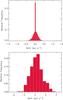 |
Fig. 1 Distribution of velocity shifts from the cross-correlation of ARGUS calibration arc spectra (top) and from the cross-correlation of nebular lines (bottom) between different epochs/exposures. |
3.2. Variability criteria
In order to exclude the stars exhibiting RV variations from our calculation of the velocity dispersion, we implemented the following quantitative assessment of the variability.
For each star and epoch, we started by fitting Gaussian profiles to individual stellar absorption lines (He ii λ4200, He ii λ4542, He i+He ii λ4026, He i λ4143, He i λ4388 and He i λ4471, or a subset when some of these lines were too weak or the S/N too low). In principle, the profiles of the He lines are not Gaussian, particularly in the wings. However, given the moderate S/N of our spectra and the noise in the line wings, the use of Gaussians provided good fits to the line profiles (see Fig. 2) and did not affect the results. We used the MPFIT idl least-squares fitting routine (Markwardt 2009) and Gaussian profiles defined by their central radial velocity, width, depth, and continuum value. An example fit is shown in Fig. 2 for the ARGUS source VFTS 1026. The resulting 1σ error on the measured RV in this case is ± 2.1 km s-1, illustrating the precision that can be achieved for a single epoch with a good quality spectrum. To check if errors in the normalisation of the continuum could influence the RV measurements, we also performed the fits allowing for a linear component instead of a constant continuum, but this did not affect the results. We chose the Gaussian fitting approach (as opposed to cross-correlation for example) because it can provide reliable error estimates on the velocities and directly yields absolute RVs, which we need to compute the velocity dispersion if different lines are used for different stars (see Sect. 3.3). This method is also well suited to our data set, for which the quality of spectra varies significantly between stars and even from one epoch to the next.
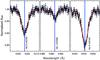 |
Fig. 2 Example of a simultaneous Gaussian fit (i.e. same RV for all lines) to the He ii λ4200, He i λ4388, and He ii λ4542 absorption lines for an individual epoch of the ARGUS source VFTS 1026 (O2-4.5 + mid/late O, see Sect. 4). |
The lines listed above are characteristic of the O-type stars composing the vast majority of our sample (see Sect. 4 and Table 1). They were the only lines generally strong enough to perform satisfying RV measurements on the spectra of individual epochs. Metallic lines were not considered because they were generally too weak, and Balmer lines were ignored because their profiles and apparent RVs can be affected by stellar winds or strong/variable nebular contamination. When one of the fitted lines appeared significantly contaminated by nebular emission it was also rejected, unless the nebular component could be clearly identified and the fit could be performed on the wings of the line only. The most affected line was He i λ4471, but it was also occasionally a problem for the other He i lines.
From close inspection of all the fitted profiles, we first identified the stars showing double-lined spectroscopic binary (SB2) profiles. Four of the 41 ARGUS sources show SB2 profiles (VFTS 1016, 1019, 1031 and 1033), and none of them had a primary component with a constant RV throughout all epochs (based on the criteria below), suggesting that they are genuine multiple systems and not just the result of the alignment of two stars with different RVs along the line of sight. The epochs at which SB2 profiles are observed in these sources are indicated in Table A.2.
We considered a star as a radial velocity variable if the series of RV measurements of any of the fitted lines of that star contained at least one strongly deviant point, which we defined as
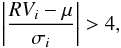 (1)where
RVi and
σi are the radial velocity and its
1σ error at epoch i, and μ is the
weighted mean RV over all the epochs. If the above condition was fulfilled for at least
one individual line, then the null hypothesis of constant RV was rejected.
(1)where
RVi and
σi are the radial velocity and its
1σ error at epoch i, and μ is the
weighted mean RV over all the epochs. If the above condition was fulfilled for at least
one individual line, then the null hypothesis of constant RV was rejected.
For each star and each line, we also computed the value of χ2
assuming a constant RV, i.e. 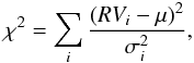 (2)and rejected the constant RV hypothesis when
the goodness of fit of a constant RV model to the data was poor, which we defined as
(2)and rejected the constant RV hypothesis when
the goodness of fit of a constant RV model to the data was poor, which we defined as
 (3)where
P(χ2,ν) is the probability
that, in a χ2 distribution with ν degrees of
freedom (ν = # of epochs − 1), the value of
χ2 is less than or equal to the value computed in Eq. (2). The thresholds adopted in Eqs. (1) and (3) were chosen so that the probability of a false variability detection in our
sample (given the sampling and accuracy of our measurements) remained negligible. In their
analysis of the multiplicity properties of the O-type stars in VFTS, Sana et al. (Paper
VIII) adopted slightly different variability criteria, but mention that their results are
generally equivalent to those of a variability test based on the goodness of fit of a
constant RV model like that of Eqs. (2) and
(3).
(3)where
P(χ2,ν) is the probability
that, in a χ2 distribution with ν degrees of
freedom (ν = # of epochs − 1), the value of
χ2 is less than or equal to the value computed in Eq. (2). The thresholds adopted in Eqs. (1) and (3) were chosen so that the probability of a false variability detection in our
sample (given the sampling and accuracy of our measurements) remained negligible. In their
analysis of the multiplicity properties of the O-type stars in VFTS, Sana et al. (Paper
VIII) adopted slightly different variability criteria, but mention that their results are
generally equivalent to those of a variability test based on the goodness of fit of a
constant RV model like that of Eqs. (2) and
(3).
As a further check, we investigated line profile variations (LPV) by computing Time Variance Spectra (TVS; Fullerton et al. 1996). The only difference with the method of Fullerton et al. (1996) is that we used the known error bars at each pixel to define a wavelength-dependent threshold instead of using a flat threshold based on continuum noise. This has the advantage of taking into account the varying S/N as a function of wavelength. The TVS at wavelength λ is given by
 (4)where N is the number of
spectra in the time series,
fi(λ) and
σi(λ) are the flux and
1σ error at wavelength λ for epoch i,
and ⟨f(λ) ⟩ is the weighted average flux of all
epochs at wavelength λ. The threshold for variability at a confidence
level of 99% is
(4)where N is the number of
spectra in the time series,
fi(λ) and
σi(λ) are the flux and
1σ error at wavelength λ for epoch i,
and ⟨f(λ) ⟩ is the weighted average flux of all
epochs at wavelength λ. The threshold for variability at a confidence
level of 99% is 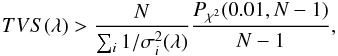 (5)where
Pχ2(0.01,
N − 1) is the cutoff value in a χ2 distribution with
N − 1 degrees of freedom such that the probability that a random
variable is greater than this cutoff value is equal to 0.01. The cases for which
significant variability is inferred from the TVS are indicated in Table A.2. These results generally confirm those obtained
from the other variability tests, and in two cases help to establish significant
variability in emission-line stars with no or only weak absorption lines. Figure 3 shows examples of TVS for two stars of our ARGUS
sample, one revealing no variability and the other showing significant LPV. Note that the
TVS often shows variability in nebular emission lines due to changes in conditions
affecting the sky subtraction, but we ignore these spectral regions when assessing the
variability of a star. The quantity TVS1/2 is plotted in Fig. 3 because it scales linearly with the size of the
spectral flux deviations and gives a direct estimate of the amplitude of the variations.
(5)where
Pχ2(0.01,
N − 1) is the cutoff value in a χ2 distribution with
N − 1 degrees of freedom such that the probability that a random
variable is greater than this cutoff value is equal to 0.01. The cases for which
significant variability is inferred from the TVS are indicated in Table A.2. These results generally confirm those obtained
from the other variability tests, and in two cases help to establish significant
variability in emission-line stars with no or only weak absorption lines. Figure 3 shows examples of TVS for two stars of our ARGUS
sample, one revealing no variability and the other showing significant LPV. Note that the
TVS often shows variability in nebular emission lines due to changes in conditions
affecting the sky subtraction, but we ignore these spectral regions when assessing the
variability of a star. The quantity TVS1/2 is plotted in Fig. 3 because it scales linearly with the size of the
spectral flux deviations and gives a direct estimate of the amplitude of the variations.
If none of the three tests above (Eq. (1), Eq. (3), TVS) revealed variability in individual lines, we performed simultaneous Gaussian fits of He ii λ4200, He ii λ4542 and He i λ4388 (or a subset of these lines when one of them was too weak or simply not present) by forcing their central RV to be the same (see Fig. 2 for an example). These three lines were adopted because they give reliable absolute RVs (see Sect. 3.3). We can therefore fit them together to obtain more precise RV measurements. The series of RV measurements resulting from these simultaneous fits were then tested for variability using Eqs. (1) and (3) again (see results in Table A.2). Stars still showing no sign of variability were then considered as suitable to study the dynamics of the cluster. The RVs of the ARGUS sources for all individual epochs are presented in Table A.3.
Out of 41 ARGUS sources, 16 are not detected as variable, 17 are variable (four SB2, 11 SB1, two emission-line stars with variability determined from the TVS), seven have a too low S/N
for a meaningful variability analysis, and another one is an emission-line star with no suitable absorption line for RV analysis and for which no significant variability was detected from the TVS.
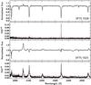 |
Fig. 3 Weighted mean spectrum (first and third panels from the top) and Temporal Variance Spectrum (TVS1/2; second and fourth panels from the top) for the ARGUS sources VFTS 1028 and VFTS 1025. The red dashed curves indicate the 99% confidence level for variability. Significant variability is only seen in the nebular emission lines of VFTS 1028, but it is detected in several stellar lines in VFTS 1025. |
3.3. Absolute radial velocities
We want to use as many lines as possible to increase the precision of RV measurements, but at the same time we need to make sure that the selected lines give accurate results. In particular, all the lines fitted simultaneously to measure the RV of a given star should give consistent results when fitted individually, and the selected lines should provide consistent absolute RVs if different subsets of lines are used for different stars (e.g. He i lines for late O-type stars and He ii lines for early O-type stars).
Our choice of suitable lines for absolute RV measurements (He i λ4388, He ii λ4200, and He ii λ4542) is supported by the RV analysis performed in Paper VIII on the large sample of O-type stars observed with Medusa (see Sect. 5). The final RVs adopted for the non-variable ARGUS stars are obtained from simultaneous fits of these three lines or a subset of them.
In stars with strong winds, wind infilling of photospheric lines can modify the RV measured by Gaussian fitting for lines like He ii λ4200 and He ii λ4542 and also result in RV shifts between these lines. Comparison of Gaussian fitting measurements and values determined from CMFGEN models shows good consistency for O-type dwarfs and giants, but small shifts of a few tens of km s-1 for supergiants (P. Crowther, priv. comm.). In our calculation of the velocity dispersion (Sect. 6.1), we therefore payed particular attention to the stars that are identified as possible supergiants (Sect. 4).
4. Spectral classification of ARGUS non-variable sources
 |
Fig. 4 Distribution of ARGUS and Medusa sources used in this work overlaid on an F555W HST-WFC3 image. ARGUS stars in which no variability was detected are shown with blue circles, ARGUS variable stars are represented by red squares, and ARGUS stars with too low S/N for RV analysis or no suitable absorption lines are indicated by red crosses. The ARGUS IFU pointings (A1 to A5) are also shown as grey transparent rectangles. Medusa non-variable stars added to the sample are represented by green diamonds. The dashed circles indicate projected radial distances of 2, 4, 6, and 8 pc from the centre of R136. |
RVs of ARGUS and MEDUSA sources showing no significant variability.
To get a general idea of the spectral content of our ARGUS sample, we classified the non-variable and presumably single stars. We did not attempt the complex task of classifying the binaries/variable stars, partly because the limited wavelength coverage of the ARGUS spectra makes it even more difficult.
To assign spectral types (SPT), we visually inspected the ARGUS spectra degraded to an effective resolving power of 4000 and, following the premises of Sota et al. (2011), we performed a morphological classification. In particular, for stars at intermediate and late subtypes, we used the eye-estimated line ratios of He i+ii λ4026 to He ii λ4200, He i λ4471 to He ii λ4542, He i λ4388 to He ii λ4542, He i λ4143 to He ii λ4200 and Si iii λ4552 to He ii λ4542 in order to assign the spectral subtype. For the hottest stars, on the other hand, we were not able to exploit the primary criteria based on the Nitrogen ionization equilibrium because our ARGUS spectra do not cover wavelengths beyond ~4570 Å. We thus concentrated on criteria related to the initial appearance of certain He i lines (such as He i λ4471, He i λ4143, and He i λ4388), and the presence and strength of N iv λ4058 and the Si iv doublet in emission. The morphological classification of our targets was furthermore constrained by comparing the degraded spectra to the spectra of O-type standards of solar metallicity compiled for the Tarantula Survey (Sana et al., in prep.) as well as to the spectra of VFTS targets obtained with Medusa-Giraffe which have already been classified.
Assigning a luminosity class to the ARGUS targets was more difficult because we could not exploit the selective emission effects in He ii λ4686 and N iii λλ4634–4640–4642 (at subtypes earlier than O8), and the value of the He ii λ4686/He i λ4713 ratio (at subtypes O9-9.7). While at late-O types one could still rely on secondary criteria, such as the ratio of Si iv λ4089 to He i λ4026, no alternative luminosity diagnostics exist at early- and mid-O types. Given this situation, we decided to follow Conti & Alschuler (1971) and exploit the increasing intensity of Si iv λ4089 relative to the nearby He i λ4143 (at subtypes later than O5 only).
The classification of the non-variable ARGUS targets, derived as outlined above, is presented in Table 1. In Sect. B of the appendix, we comment on specific sources, in particular those that have revised spectral types and the three that appear to have composite spectra. The accuracy of the spectral types reported in Table 1 for the ARGUS sources is typically between one and one and a half subtypes, with uncertainties caused by the effects of nebular emission, rotation (Markova et al. 2011), and metallicity (Markova et al. 2009). The uncertainty on the luminosity class is significantly larger as we were only able to separate the stars into two broad categories: high luminosity objects (luminosity class I/II) and low luminosity objects (luminosity class III/V). For completeness, we also include previously published spectral types in Table 1.
5. Supplementary Medusa data
To complement our RV measurements of the ARGUS sources, we also include the RV measurements of the non-variable O-type stars observed with Medusa-Giraffe (Paper VIII) in the inner 10 pc of R136. This gives us 22 additional stars, 20 of which are located between 5 and 10 pc from the centre of the cluster. We do not consider stars beyond 10 pc from the centre in our analysis of R136. Although somewhat arbitrary, this cutoff at 10 pc is a reasonable trade-off between increasing the number of stars in our sample and limiting the possible contamination from nearby clusters or other star formation events in the surroundings of R136.
The Medusa observations (see Paper I) were performed using three of the standard Medusa-Giraffe settings (LR02: λ = 3960–4564 Å, Δλ = 0.61 Å, R ~ 7000; LR03: λ = 4499–5071 Å, Δλ = 0.56 Å, R ~ 8500; HR15N: λ = 6442–6817 Å, Δλ = 0.41 Å, R ~ 16 000). To detect RV variables, six epochs were observed for the LR02 setting with time constraints similar to those of the ARGUS observations (Sect. 2 and Table A.1).
The RV and variability analysis of these stars is presented in Paper VIII in the context of a study of the multiplicity of O-type stars in 30 Dor. The method is similar to the one we applied in Sect. 3.2. As a consistency check, we applied our method on the LR02 Medusa spectra of several O-type stars and found absolute RVs and 1σ uncertainties fully consistent with the results from Paper VIII. Thus, we do not repeat all the RV measurements of the Medusa stars, but adopt the values of Paper VIII instead. For two of those additional Medusa stars, the luminosity class could not be constrained, but none of the others is classified as a supergiant (Walborn et al., in prep.). The RVs of these stars, obtained from Gaussian fitting, should therefore be reliable as discussed in Sect. 3.3. The spectral types of the non-variable Medusa O-type stars, determined by Walborn et al. (in prep.), are listed in Table 1.
Note that in parallel to the ARGUS observations, a few stars were also observed in the inner 10 pc of R136 with the Ultraviolet and Visual Echelle Spectrograph (UVES), providing a greater resolving power than the Giraffe spectrograph. All the UVES targets but one in this region were also observed with ARGUS or Medusa, and these were already shown to be binaries/variable based on the ARGUS or Medusa observations alone. One star was observed only with UVES; Mk 39, an O2.5 If*/WN6 star (Crowther & Walborn 2011), which is not suitable for our RV analysis because the He ii lines are wind contaminated.
Our final sample of apparently single ARGUS and Medusa stars within 10 pc from the centre of R136 is presented in Table 1. These are all the stars that we use for the analysis of the dynamics in the following sections. Their absolute RVs and their projected distance from the centre of the cluster (which we adopt to be the position R136-a1) are also listed. The projected distances are for an adopted distance modulus of 18.5 mag (see Paper I). The absolute RV adopted for a given star is the weighted mean RV of all epochs. The spatial distribution of variable and non-variable ARGUS sources is shown in Fig. 4, along with the positions of the non-variable Medusa O-type stars added to our sample.
6. Velocity dispersion
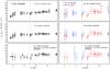 |
Fig. 5 Observed line-of-sight velocity dispersion, as a function of R, for the stars within a projected radial distance R from the centre of R136. In the left panels, stars of all subtypes are included, while in the right panels, we divide them into two subsamples: O7 and earlier (blue triangles), O8 and later (red squares). In the top panels, all the non-variable stars (see Table 1) are included. In the middle panels, two stars with a radial velocity more than 3σ away from the mean RV are excluded. In the bottom panel, supergiant and SB2 candidates are also excluded. In each panel (and subsample), the first point from the left is the velocity dispersion of the four stars (of that subsample) closest to the centre, the second point is the velocity dispersion of the innermost five stars, and so on. |
6.1. Velocity dispersion upper limit
We can now determine the observed line-of-sight velocity dispersion (σ1D) from the RV measurements of the non-variable stars. Because any effect not yet taken into account (e.g. undetected binaries, intrinsic errors) would tend to increase the inferred σ1D, we can consider that the results shown in this subsection represent an upper limit to the actual line-of-sight velocity dispersion of the cluster.
In what follows, σ1D is determined by computing the standard
deviation, i.e. (Bevington 1969) 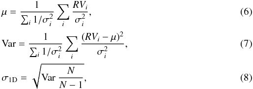 where
σi is the uncertainty on the RV
measurement RVi,
μ is the weighted mean RV, Var is the variance, and N
is the number of measurements.
where
σi is the uncertainty on the RV
measurement RVi,
μ is the weighted mean RV, Var is the variance, and N
is the number of measurements.
In the upper left panel of Fig. 5, we present, as a function of projected radial distance from the centre of R136, the σ1D of all the non-variable stars within that radius. Apart from an apparent increase in σ1D in the inner region (most likely due to the low number of stars and associated large uncertainty on σ1D and its error), the velocity dispersion profile is relatively flat. For the stars within 5 pc from the centre, we find σ1D ≲ 6 km s-1. Two stars dominate the increase in σ1D between 5 and 10 pc: VFTS 536 (rd = 7.2 pc; RV = 248.4 ± 1.4 km s-1) and VFTS 540 (rd = 8.3 pc; RV = 242.7 ± 1.1 km s-1).
As a next step, to see the effect of possible outliers (slow runaways or massive stars along the line of sight but not members of R136), we exclude the stars with an RV more than 3σ away from the (weighted) mean RV of our sample (267.7 km s-1). We choose σ to be 6 km s-1, the observed dispersion of the stars within 5 pc from the centre. VFTS 536 and VFTS 540 are indeed >3σ outliers, and excluding them results in an even flatter profile (Fig. 5, middle left panel).
When also excluding possible supergiants (I/II or no luminosity class attributed in Table 1), for which the RVs obtained from Gaussian fits could be problematic (see Sect. 3.3), and SB2 candidates (composite spectra, see Table 1), the results do not change significantly, although more fluctuations are seen in the profile and the error bars are larger due to the smaller number of stars (Fig. 5, bottom left panel). The apparent increase in the inner 2–3 pc also disappears when these supergiant and SB2 candidates are excluded.
In Sect. 6.5, we estimate the contribution of errors and undetected binaries to σ1D and attempt to reproduce the observed velocity dispersion for the stars within 5 pc (in projection) from the centre, i.e. σ1D = 6 km s-1. We could choose a different radius, but because the velocity dispersion profile appears remarkably flat in the inner 10 pc, this would not change the results significantly. There is also a natural cut at ~5 pc if we consider the definition of a cluster proposed by Gieles & Portegies Zwart (2011), which states that stellar agglomerates for which the age of the stars exceeds the crossing time are bound and thus referred to as star clusters. The crossing time (i.e. the distance for a star to travel from one side of the cluster to the other; 2r) is roughly σ1D × age. Given an age of ~2 Myr and σ1D ~ 6 km s-1, we can conclude that the stars that are physically within ~6 pc from the centre are part of the cluster following the above definition.
6.2. Contamination by “halo” stars
The light profile of R136 suggests that it is not a single-component cluster but the composite of a real cluster and a “halo”, i.e. an OB association, with the latter contributing to more than 50% and possibly as much as 90% of its total integrated light (Maíz-Apellániz 2001; Mackey & Gilmore 2003). It is therefore worth asking how much could the OB association contaminate our velocity dispersion measurement for the cluster. In the double-component EFF fit (Elson et al. 1987) to the light profile of R136 by Mackey & Gilmore (2003), the projected radius where the two components contribute equally is at about 5 pc. If we consider the inner profile as the cluster and the outer profile as the halo, we can conclude from this fit that the contribution of halo stars projected on the cluster is negligible (≲ 5%) in the inner 1.25 pc, but it could be significant beyond 5 pc.
We might expect the OB association to have a low velocity dispersion, as is observed in Galactic cases once binaries and runaways are excluded (e.g. de Bruijne 1999). However, the latter are hard to identify if there is a massive cluster with a higher velocity dispersion embedded in the OB association. To explore the cluster/halo dichotomy, we divided our sample into two subtype groups such that they had roughly the same number of stars, which resulted in these two subsamples: earlier than O7 and later than O8. We then computed the velocity dispersion as in Sect. 6.1 for the stars that could be placed in one of these groups (Fig. 5, right panels). We would expect the earlier type stars to be more concentrated towards the centre as a result of mass segregation or due to an overall age difference between the cluster and halo populations. Figure 5 indeed suggest a higher concentration of early-types towards the core, but this could well be due to the increasing crowding effects in the innermost regions favouring the detection of the brightest (most probably earliest) stars. In any case, there is no obvious difference in velocity dispersion between the two subsamples, and the contribution of halo stars to the velocity dispersion remains very difficult to identify.
6.3. The contribution of cluster rotation
In an accompanying letter (Hénault-Brunet et al. 2012), we present evidence for rotation of R136. From comparison of our RV measurements with different simple rotating models, we infer a rotational amplitude of ~3 km s-1 and an optimal position angle for the rotation axis at an angle of ~45° east of north. To remove the anisotropy due to the suggested rotation and its contribution to the computed velocity dispersion, we subtracted from our measured RVs the rotation curve from these simple models. We find that the velocity dispersion obtained after this correction is typically 0.5 km s-1 lower than the values presented in Sect. 6.1. Thus, a small component of the observed line-of-sight velocity dispersion could be attributed to cluster rotation.
6.4. The velocity dispersion when including binaries/variable stars
It is interesting to see what the computed σ1D would have been if we had not been careful about identifying and rejecting binaries and variable stars, or if we were not dealing with multi-epoch observations.
We randomly selected one epoch for each ARGUS source on which the RV analysis was performed (variable and non-variable sources), and repeated the process for 10 000 combinations of epochs. A median σ1D of 25.0 km s-1 was obtained from all these combinations of single-epoch RV measurements, with a standard deviation of 5.9 km s-1 and values of σ1D ranging from 12.9 to 48.0 km s-1. If we do a similar test but limit ourselves to the non-variable ARGUS sources (Table 1), we find a median σ1D of 6.2 km s-1 (in good agreement with the results of Sect. 6.1), with a standard deviation of 0.7 km s-1.
Note however that the velocity dispersion obtained when including all the RV variables cannot be directly compared with the velocity dispersion one would obtain from the integrated light of a distant star cluster, as a few outliers could increase the velocity dispersion significantly without contributing much to the integrated light.
6.5. The contribution of errors and undetected binaries
To estimate the contribution of measurement errors and undetected binaries to the observed velocity dispersion, we performed a series of Monte Carlo simulations. These are adapted from the method presented by Sana et al. (2009) and refined in Paper VIII to estimate the probability to detect binary systems. Bosch & Meza (2001) have also previously performed similar Monte Carlo simulations testing intrinsic and observed properties of binary stars. Our simulations mimic the process that we have been going through, i.e. identify variables from series of RV measurements and then compute the velocity dispersion from the remaining non-variable stars.
The general procedure goes as follows. We first adopt reasonable orbital parameter distributions (period, mass ratio, eccentricity) and an intrinsic binary fraction. Then, for 10 000 populations of N stars (where N is the size of the sample, i.e. all the ARGUS sources plus Medusa O-type stars within 5 pc from the centre of R136 on which the RV variability analysis was performed), we randomly draw which are binaries and which are single, and also randomly draw the parameters for the binaries from the adopted distributions. From these, we compute the orbital velocity at each epoch (based on the time sampling of the observations) for all the binaries assuming random orientations of the orbital planes and uncorrelated random time of periastron passage. We then add the measurement noise (based on the RV uncertainties of our sample) to the computed RVs of binaries and single stars. By applying the RV variability criteria of Sect. 3.2, we can then eliminate the stars that we would have flagged as variable, compute the line-of-sight velocity dispersion of the apparently non-variable stars, and estimate the contribution from the orbital motion of binaries that were not detected. This procedure has the advantage that we not only take into account the long period binaries (i.e. too long a period to be detected with the VFTS), but also all the shorter binary systems missed by our time sampling, with a statistical weight exactly defined by the incompleteness.
Before performing the full procedure outlined above, we estimated the contribution of measurement errors by taking a population with no binaries. For each star, we drew the RV at each epoch from a Gaussian distribution centred on zero and a sigma corresponding to the RV error at the corresponding epoch. We then applied the RV variability criteria of Sect. 3.2 to make sure that our adopted thresholds do not lead to false detections (the false detection rate was indeed found to be negligible). We finally computed the velocity dispersion of the population and repeated this for 10 000 populations. The resulting velocity dispersion distribution is represented by the blue dotted curve in Fig. 6. The peak of this blue curve is at 0.80 (km s-1)-1, out of the graph. It shows that, given the precision of our RV measurements, the intrinsic contribution of errors to the observed velocity dispersion is small. Note that we performed two tests on the population size: (i) we first used N stars, the full population size; and (ii) we randomly picked stars from the initial population following the results of a binomial test with a success rate of 50%, mimicking the fact that the dispersion is usually computed using an effective population of about half the original one because of binary rejection. The two approaches made no difference on the resulting contribution of measurement errors.
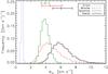 |
Fig. 6 Estimate of the line-of-sight velocity dispersion distribution for massive stars in the inner 5 pc of R136. The blue dotted curve shows the contribution of measurement errors. The red dashed curve is the distribution from binaries undetected after applying our variability criteria (the initial input population has a binary fraction of 100%, and an Öpik-law distribution of the periods is adopted with period range of 0.15−6.85 in log P with P in units of days). The green solid curve is the dynamical velocity dispersion which best reproduces the observed velocity dispersion. The black solid curve takes into account measurement errors, undetected binaries, and the dynamical velocity dispersion. The median (central tick) and 68% confidence interval (equivalent to ± 1 σ for Gaussian distributions) of the distributions are indicated on the upper part of the graph. |
The contribution of undetected binaries depends on what is assumed for the input distributions. We focus here on the distribution of orbital periods, because the distributions of mass ratios and eccentricities have a limited impact (see Paper VIII). In what follows we adopt a flat distribution of mass ratios, as motivated by the recent results of Sana & Evans (2011), Sana et al. (2012a), and Kiminki & Kobulnicky (2012).
As a first test to estimate the intrinsic contribution of undetected binaries, we adopted
a conservative binary fraction of 100% and a standard Öpik-law distribution for the period
(i.e. flat distribution of log P) with a period range of 0.15−6.85 (in
log P, where P is in units of days). The maximum
period adopted corresponds to the extrapolation of the Öpik law until a 100% binary
fraction is reached when considering the observed binary fraction and the overall
detection rate of VFTS (Paper VIII). We ran the full procedure outlined above, but without
adding the measurement noise to the extracted orbital velocities. The resulting velocity
dispersion distribution (from the stars that are not identified as RV variable) is shown
with the red dashed curve in Fig. 6. Under these
assumptions, the velocity dispersion from undetected binaries is
 km s-1. The quoted value is
the median of 10 000 populations, and uncertainties correspond to the 68% confidence
interval (equivalent to ± 1σ for Gaussian distributions). Note that
within uncertainties, the undetected binaries alone can produce the observed velocity
dispersion of 6 km s-1.
km s-1. The quoted value is
the median of 10 000 populations, and uncertainties correspond to the 68% confidence
interval (equivalent to ± 1σ for Gaussian distributions). Note that
within uncertainties, the undetected binaries alone can produce the observed velocity
dispersion of 6 km s-1.
To recover the true velocity dispersion of the cluster, we repeated the simulation, this
time adding the measurement noise to the orbital RVs. We also included a contribution from
the dynamical velocity dispersion that was varied until the most probable velocity
dispersion matched the observed velocity dispersion. For simplicity, we assumed that this
dynamical contribution to the velocity dispersion did not vary as a function of radius. We
estimate that the line-of-sight velocity dispersion attributable to the cluster dynamics
is  km s-1. The errors on this
value correspond to changes in the input dynamical velocity dispersion that result in
median values of the output velocity dispersion distribution at percentiles 0.16 and 0.84
of the optimal output distribution (i.e. the “overall” simulated distribution for which
the median is the observed velocity dispersion). Note that we obtain a velocity dispersion
of 26 ± 9 km s-1 from these simulations for a single epoch when including
all binaries (i.e. without applying our variability criteria and thus without rejecting
the binaries that would be detected), in keeping with the value of
~25 km s-1 that we found in Sect. 6.4 from the single-epoch RV measurements of all ARGUS sources (variable and
non-variable).
km s-1. The errors on this
value correspond to changes in the input dynamical velocity dispersion that result in
median values of the output velocity dispersion distribution at percentiles 0.16 and 0.84
of the optimal output distribution (i.e. the “overall” simulated distribution for which
the median is the observed velocity dispersion). Note that we obtain a velocity dispersion
of 26 ± 9 km s-1 from these simulations for a single epoch when including
all binaries (i.e. without applying our variability criteria and thus without rejecting
the binaries that would be detected), in keeping with the value of
~25 km s-1 that we found in Sect. 6.4 from the single-epoch RV measurements of all ARGUS sources (variable and
non-variable).
We also ran simulations using different binary fractions and period distributions. We first considered only periods shorter than 103.5 days, i.e. the ones that could be detected by VFTS (Paper VIII). Assuming a 50% binary fraction and a standard Öpik law for the period distribution, the estimated velocity dispersion from the undetected shorter period binaries alone is 2.4 + 1.5-1.0 km s-1. If instead of the Öpik law we adopt the distribution measured in Paper VIII for the VFTS O-type binaries (f(log P) ∝ (log P)-0.45), we obtain a velocity dispersion from the undetected shorter period binaries of 2.0 + 1.4-0.9 km s-1. This is the minimal contribution of undetected binaries. These values (to be compared with the red dashed curve in Fig. 6) indicate that the contribution of undetected binaries is dominated by long period systems outside the sensitivity range of the VFTS.
Recall that the velocity dispersion from undetected binaries when including very long
period systems as well (i.e. binary fraction 100%, Öpik-law distribution of periods
ranging from 0.15 to 6.85 in log P) is
km s-1. If we adopt the
distribution with
f(log P) ∝ (log P)-0.45
instead, the velocity dispersion from both short and long period undetected binary systems
is  km s-1. In that case, the
dynamical velocity dispersion that best reproduces the observed velocity dispersion would
be 5 km s-1. The Öpik law might therefore overestimate the contribution of
binaries by ~1 km s-1 compared to the period distribution measured in
VFTS O-type binaries (Paper VIII), but we should bear in mind that the extrapolation of
the period distribution to long periods is very uncertain.
km s-1. In that case, the
dynamical velocity dispersion that best reproduces the observed velocity dispersion would
be 5 km s-1. The Öpik law might therefore overestimate the contribution of
binaries by ~1 km s-1 compared to the period distribution measured in
VFTS O-type binaries (Paper VIII), but we should bear in mind that the extrapolation of
the period distribution to long periods is very uncertain.
In summary, we estimate that the velocity dispersion due to cluster dynamics alone (i.e. removing the effect of binarity but still including a small contribution from rotation) is likely somewhere between 4 and 5 km s-1, with a contribution of ~0.5 km s-1 from rotation (see Sect. 6.3).
7. Discussion
Now that we have our measurement of the velocity dispersion at hand we can test the
hypothesis that the cluster is in virial equilibrium. This is often done by deriving a
dynamical, or virial mass, from the velocity dispersion which is then compared to the
photometrically determined mass. To be able to derive the former we require knowledge about
the mass distribution of the stars. For equilibrium models with an isotropic velocity
dispersion the one-dimensional velocity dispersion, σ1D, relates
to the mass, M, and the virial radius, rv, as
 . The virial radius is defined as
rv ≡ GM2/(2W),
with W the potential energy of the system. This relation is often expressed
in terms of the radius containing half the light in projection, or effective radius
(reff), as
. The virial radius is defined as
rv ≡ GM2/(2W),
with W the potential energy of the system. This relation is often expressed
in terms of the radius containing half the light in projection, or effective radius
(reff), as  , with η ≈ 10. This is under
the assumption that light traces mass, that the half-mass radius
(rh) in projection is 3/4 times the 3D half-mass radius (Spitzer 1987) and that the ratio
rv/rh ≈ 5/4. The first two
assumptions are not valid when a cluster is mass segregated (Fleck et al. 2006) as the 2D light radius can be twice as small
as the 3D mass radius (Gaburov & Gieles
2008; Hurley 2007). For models with very
flat density profiles, it is difficult to estimate the half-light radius. The surface
brightness profiles of young clusters are often approximated by cored templates with a
power-law decline of the form
, with η ≈ 10. This is under
the assumption that light traces mass, that the half-mass radius
(rh) in projection is 3/4 times the 3D half-mass radius (Spitzer 1987) and that the ratio
rv/rh ≈ 5/4. The first two
assumptions are not valid when a cluster is mass segregated (Fleck et al. 2006) as the 2D light radius can be twice as small
as the 3D mass radius (Gaburov & Gieles
2008; Hurley 2007). For models with very
flat density profiles, it is difficult to estimate the half-light radius. The surface
brightness profiles of young clusters are often approximated by cored templates with a
power-law decline of the form  , where r0 is a
scale radius. These profiles are often referred to as EFF profiles (Elson et al. 1987). For γ > 2 these models contain a
finite amount of light, but diverge to infinite luminosity when γ ≤ 2. The
boundary at γ = 2 corresponds to 3D light profiles that decline as
r-3. For γ larger than, but close to 2, the
ratio rv/rh becomes very sensitive
to the exact value of γ (Portegies Zwart
et al. 2010). Additionally, determining reff becomes
difficult as this quantity, and the total luminosity, can become unrealistically large when
extrapolating to infinity.
, where r0 is a
scale radius. These profiles are often referred to as EFF profiles (Elson et al. 1987). For γ > 2 these models contain a
finite amount of light, but diverge to infinite luminosity when γ ≤ 2. The
boundary at γ = 2 corresponds to 3D light profiles that decline as
r-3. For γ larger than, but close to 2, the
ratio rv/rh becomes very sensitive
to the exact value of γ (Portegies Zwart
et al. 2010). Additionally, determining reff becomes
difficult as this quantity, and the total luminosity, can become unrealistically large when
extrapolating to infinity.
The light profile of R136 has a profile close to γ = 2 (McLaughlin & van der Marel 2005), with indications for a “bump” in the optical light profile at about 10 pc (Hunter et al. 1995; Maíz-Apellániz 2001; Mackey & Gilmore 2003). The presence of an additional component from the larger scale and near-constant-density OB association in which R136 is located (see Sect. 6.2) has been interpreted as the reason for this relatively flat profile. In the near-infrared (NIR), the profiles are even flatter than the critical value (Andersen et al. 2009; Campbell et al. 2010) and the halo structure is not that obvious, but the NIR data did not extend very far into the OB association. Mass segregation, age differences between the core and halo, and differential extinction (which becomes important ~10 pc away from the centre of R136) could explain the flatter profile in the NIR compared to the optical.
With the above caveats in mind, it is still interesting to see what dynamical mass we obtain for R136. If we assume η ≈ 10, 3.4 ≲ σ1D ≲ 6.0 km s-1 (Sect. 6), and adopt a half-light radius of reff = 1.7 pc (Hunter et al. 1995) which is consistent with the half-light radius obtained for the inner component of the double EFF fit discussed in Sect. 6.2, we get M = 4.6−14.2 × 10⁴ M⊙. This is consistent with the estimated photometric mass of ~105 M⊙ by Andersen et al. (2009), for which the cluster mass of ~5 × 10⁴ M⊙ (computed for stellar masses between 25 M⊙ and down to 2.1 M⊙) was extrapolated assuming a Salpeter slope down to 0.5 M⊙.
However, because of the difficulties outlined above, we decide to address whether R136 is
in virial equilibrium by exploring an alternative method for which we do not need to know
the total mass. This relies on estimating the central velocity dispersion by following a
very similar method to that presented by Richstone &
Tremaine (1986). From the observations we find that the velocity dispersion is
roughly constant with radius (Sect. 6.1). We can
express the expected central dispersion σ1D(0) of
(self-consistent and isotropic) models with isothermal inner parts in terms of observed
properties of the cluster  (9)where
  is the gravitational constant,
ΥV the mass-to-light ratio in
M⊙/L⊙ in the
V-band and α depends on the model.
is the gravitational constant,
ΥV the mass-to-light ratio in
M⊙/L⊙ in the
V-band and α depends on the model.
We first consider the modified Hubble profile (Rood et al.
1972), which is an EFF profile with γ = 2, very close to the best
fit to the surface brightness profile in the optical. From solving Jeans’ equations assuming
hydrostatic equilibrium and isotropic velocities we find that
α = 3−4ln(2) ≈ 0.227. Secondly, we look at the Plummer (1911) model for which α = 1/6 ≈ 0.167. Finally,
we can consider the isothermal sphere, which cannot be expressed in an EFF profile. For this
model r0 is defined as1![\hbox{$\rs^2=9\dispsq/[4\pi G\rho(0)]$}](/articles/aa/full_html/2012/10/aa19471-12/aa19471-12-eq113.png) , where ρ(0) is the central
density. For the isothermal sphere
I(0) ≈ 2ρ(0)r0/ΥV
(Binney & Tremaine 1987) and we thus have
α ≈ 2/9 ≈ 0.222. In conclusion, α ≈ 0.2 and the value is
relatively insensitive to the choice of model (compared to η).
, where ρ(0) is the central
density. For the isothermal sphere
I(0) ≈ 2ρ(0)r0/ΥV
(Binney & Tremaine 1987) and we thus have
α ≈ 2/9 ≈ 0.222. In conclusion, α ≈ 0.2 and the value is
relatively insensitive to the choice of model (compared to η).
The central surface brightness in the V-band is about I(0) ≈ 2.5 × 10⁶ L⊙ pc-2 (McLaughlin & van der Marel 2005) and together with r0 ≈ 0.3 pc and ΥV ≈ 0.014 (Mackey & Gilmore 2003; McLaughlin & van der Marel 2005) we find a predicted central velocity dispersion of σ1D ≈ 5.3 km s-1. Our measured dispersion is consistent with this value and we conclude that R136 is in virial equilibrium in the inner 5 pc. This is also consistent with a normal stellar initial mass function (IMF) for R136 (Andersen et al. 2009), as the expected velocity dispersion would be a factor of a few lower, for example, if the IMF was truncated at the low-mass end (the mass-to-light ratio would be lower in that case).
The expected velocity dispersion should actually be corrected for the fact that our stars are not at the centre of the cluster, unless we consider the cluster as an isothermal sphere in which case the dispersion is the same everywhere. For the Plummer model and the modified Hubble profile, the velocity dispersion for an isotropic model decreases with radius. For example, in the modified Hubble profile, the velocity dispersion at 5 pc should be ~40% lower than at the centre for a core size of 0.3 pc, so in virial equilibrium we would expect to measure a dispersion of ~3 km s-1 at 5 pc, which is still in relatively good agreement with our measured dispersion.
Other effects that we have not taken into account could also influence our estimate of the expected velocity dispersion in virial equilibrium. Mass segregation, for example, would result in a higher central surface brightness, a smaller core size, and a lower mass-to-light ratio. It is however not clear what would be the net effect on the velocity dispersion. Radial anisotropy would make the (projected) velocity dispersion profile decline more at larger radii with respect to an isotropic model with the same density profile (Clarkson et al. 2012; Wilkinson et al. 2004). On the other hand, tangential anisotropy could flatten the profile by reducing σ1D in the core and increasing it in the outer parts, which is an interesting perspective considering the evidence for rotation (Hénault-Brunet et al. 2012) and the relatively flat velocity dispersion profile that we obtained for R136. A similarly flat profile was also found for the Arches cluster albeit within a much smaller radial extent (Clarkson et al. 2012). Detailed numerical modelling of R136 is required for a meaningful quantitative discussion of the complicated effects outlined above, but this is beyond the scope of the present paper.
Other young massive clusters have recently been found to have a low velocity dispersion, suggesting that they are virial or even subvirial. Velocity dispersions of 4.5 ± 0.8 km s-1 and 5.4 ± 0.4 km s-1 were reported, respectively, for NGC 3603 (Rochau et al. 2010) and the Arches cluster (Clarkson et al. 2012) using proper motion measurements. From RV measurements of five yellow hypergiants and one luminous blue variable in Westerlund 1 showing little RV variations over 2 to 3 epochs, Cottaar et al. (2012) estimated the velocity dispersion of this cluster to be 2.1 + 3.3-2.1 km s-1. From single-epoch near-infrared spectroscopy, Mengel & Tacconi-Garman (2007) found 5.8 ± 2.1 km s-1 for the same cluster from the RVs of four red supergiants, 8.4 km s-1 from ten post-main-sequence stars (Mengel & Tacconi-Garman 2008), and finally 9.2 km s-1 from a sample of four red supergiants, five yellow hypergiants, and one B-type emission-line star (Mengel & Tacconi-Garman 2009). Note that these studies of Westerlund 1 use stars of spectral types and luminosity classes that are known to be pulsators or intrinsic RV variables (e.g. Ritchie et al. 2009; Clark et al. 2010), which along with the small number statistics (both in terms of number of stars and number of epochs) might explain the range of values obtained for the velocity dispersion.
Given the young age of these clusters for which low velocity dispersions were found, including R136, this might look somewhat surprising if we expect the clusters to be expanding following gas expulsion. However, if the age of a cluster is at least few crossing times it might have had time to re-virialize, in which case the low velocity dispersions measured are not so surprising. A consequence of these results is that these young massive clusters are certainly not being disrupted by gas expulsion, and in fact appear to be stable from a very young age. From now on, gas expulsion will not have a large effect on the dynamical evolution of the cluster. A gas-free cluster in virial equilibrium is therefore a reasonable initial condition for dynamical simulations. The gas expulsion scenario would also predict strong radial orbits in the outer parts of the cluster, which would result in a steep decline in σ1D (Clarkson et al. 2012; Wilkinson et al. 2004), and this is not observed. Several factors could potentially explain this apparent unimportance of gas expulsion in early cluster evolution, including a high star-formation efficiency (e.g. Goodwin & Bastian 2006), the formation of these clusters from the merging of dynamically cool (subvirial) substructures (e.g. Allison et al. 2009), and/or a cluster formation process resulting in a de-coupled distribution of gas and stars that offsets the disruptive effect of gas expulsion (e.g. Fellhauer et al. 2009; Moeckel & Clarke 2011; Kruijssen et al. 2012). Another consequence of these results is that even if it were true that gas expulsion had a significant effect ~1 Myr ago, then R136 would have had to be incredibly dense in the past.
R136 is often considered as an extremely dense cluster, but it is interesting to compare the low velocity dispersion that we found to the much larger line-of-sight velocity dispersion of a globular cluster like 47 Tucanae (11.6 km s-1; McLaughlin et al. 2006). R136 is still very young, and it will loose mass and expand due to stellar evolution. For an adiabatic mass loss, the radius will grow as 1/M, so the velocity dispersion will go down by at least a factor of two (σ1D ∝ (M/r)1/2 ∝ M), but in reality there is going to be even more significant expansion (Gieles et al. 2010a) which will reduce the velocity dispersion even more by the time R136 is as old as 47 Tucanae.
8. Conclusions
In an effort to determine the dynamical state of the young massive cluster R136, we used multi-epoch spectroscopy of stars in the inner regions of 30 Dor. We measured RVs with a Gaussian fitting procedure on selected key helium lines and performed a quantitative assessment of the variability. Out of 41 sources for which spectra were extracted from the ARGUS IFU data cubes, 16 were identified as non-variable. All of these were classified as O-type stars, three of which were also revealed to have composite spectra. To this sample of 16 ARGUS sources, we added measurements from 22 apparently single stars observed in the surrounding regions with Medusa-Giraffe, also as part of VFTS.
Using this sample of 38 non-variable massive stars within 10 pc from the centre of R136, we computed the velocity dispersion of the cluster. For the stars within 5 pc, we place an upper limit of 6 km s-1 on the line-of-sight velocity dispersion. This result does not change significantly if we exclude the few 3σ outliers, supergiant candidates, and stars having composite spectra. We also noted that the measured velocity dispersion of the cluster includes a small contribution of ~0.5 km s-1 from rotation.
From Monte Carlo simulations, we established that the contribution of measurement errors to the observed velocity dispersion is almost negligible. We also estimated the contribution of undetected binaries, which is relatively small and dominated by long period systems beyond the detectability range of VFTS. When taking errors and undetected binaries into account, we estimate that the true velocity dispersion of the cluster (i.e. attributable only to cluster dynamics) is between 4 and 5 km s-1 for the stars within 5 pc from the centre.
Under basic assumptions, the expected central velocity dispersion in virial equilibrium was found to be ≈ 5.3 km s-1, in good agreement with our measurement, and we conclude that R136 is in virial equilibrium. Combined with the low velocity dispersions found in a few other young massive clusters, our results suggest that gas expulsion does not significantly alter the dynamics of these clusters.
We would have obtained a velocity dispersion of ~25 km s-1 if binaries had not been identified and rejected, which supports the suggestion that the alleged super-virial state of young star clusters can be explained by the orbital motions of binary stars (Gieles et al. 2010b).
Online material
Appendix A: Individual epochs and summary of radial velocity/variability analysis
Individual epochs of the ARGUS observations.
Results of the variability tests for the ARGUS sources.
RVs (in km s-1) for individual epochs for all the ARGUS sources suitable for RV analysis.
Appendix B: Notes on individual ARGUS sources
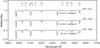 |
Fig. B.1 Non-variable ARGUS sources displaying composite spectra. Emission lines labelled are N iv λ4058 and Si iv λλ4089, 4116. Absorption lines labelled are He i λ4026, He i λ4143, He ii λ4200, He i λ4388, He i λ4471, He ii λ4542 and a diffuse interstellar band at 4428 Å. |
We comment here on selected individual sources, paying particular attention to sources with previous identifications, composite spectra, and also to those which appear multiple in the WFC3 image.
-
VFTS 542: this star is identified as a definite variable with a largeamplitude from both ARGUS and Medusa observations. ItsHe ii λ4200 and He ii λ4542 lines show a weak P Cygni component and it is classified as O2 If*/WN5 (Paper I), so even if it was not variable, its absolute RV could not be trusted. RV discrepancies as large as ~40 km s-1 are found at some epochs between He ii λ4200 and He ii λ4542.
-
VFTS 545: it is also known as Mk35 (Melnick 1985) and classified as O2 If*/WN5 (Paper I). There is a discrepancy of ~20 km s-1 between He ii λ4200 and He ii λ4542, and its absolute RV also cannot be trusted. Low-amplitude variability is only detected in He ii λ4542, which is stronger and has smaller RV uncertainties compared to He ii λ4200.
-
VFTS 570: the ARGUS spectra of this source were not analysed for RV variability because their S/N was too low, but from the Medusa spectra it was found to be a definite RV variable with a large amplitude (Paper VIII). Two stars appear to contribute significantly to the ARGUS source when comparing with the WFC3 image.
-
VFTS 585: this source was also found to be variable from the Medusa spectra (Paper VIII). Significant RV variability was detected from the relatively low S/N ARGUS spectra only once He ii λ4200 and He ii λ4542 were fitted simultaneously.
-
VFTS 1001: this source corresponds to a known Wolf-Rayet star, R134 (Feast et al. 1960), classified as WN6(h) (e.g. Massey & Hunter 1998). Although it was detected as an X-ray source and suggested as a possible colliding-wind binary by Portegies Zwart et al. (2002), it is not known to be a binary. Interestingly, our TVS analysis reveals significant variability in the He ii λ4542 emission, but it is unclear if this is due to a normalisation problem in a spectral range dominated by several emission lines, where the continuum is harder to define.
-
VFTS 1003: this source was found to be a new B[e]-type star in Paper I. The TVS analysis performed in the present work did not reveal any significant variability other than in the nebular emission lines (due to sky subtraction).
-
VFTS 1004: the WFC3 image suggests that two sources are contributing to VFTS 1004, but it does not display a composite spectrum, it is not found to be variable, and the He i λ4388, He ii λ4200 and He ii λ4542 lines all have consistent absolute RVs.
-
VFTS 1007: similarly to VFTS 1004, VFTS 1007 appears multiple when inspecting the WFC3 image, but it is not variable, it does not have a composite spectrum, and He i λ4388, He ii λ4200 and He ii λ4542 all have consistent absolute RVs.
-
VFTS 1014: the presence of N iv λ4058 and Si iv λ4089/4116 emission together with weak but well developed He i singlet lines at 4121, 4143 and 4388 Å suggests a composite spectrum (see Fig. B.1). Based on the helium line diagnostics and the absence of Si iii λ4552, the later component is identified as a mid/late O-type star. From the relative strength of N iv and Si iv, the other component is O2-4.5 (we cannot be more precise because our the ARGUS spectrum does not include the N v absorption region), in agreement with the O3 V classification of Massey & Hunter (1998). Even though its spectrum appears composite, this source did not show significant variability. The He i λ4388, He ii λ4200 and He ii λ4542 lines all have consistent absolute RVs.
-
VFTS 1015: this source is clearly multiple by comparison with the WFC3 image and significant RV variability is found in He ii λ4542. For some epochs, the RV of the He i λ4388 line is clearly different from that of He ii λ4200 and He ii λ4542 lines.
-
VFTS 1017: this source is variable. Its He ii λ4200 and He ii λ4542 lines have a weak P Cygni component. A discrepancy of up to ~30 km s-1 is found in the RVs of He ii λ4200 and He ii λ4542 at different epochs.
-
VFTS 1018: the presence of weak N iv λ4058 and Si iv λ4116 emission in combination with weak but well developed He i singlet lines suggests a composite spectrum (see Fig. B.1). Based on the helium line diagnostics and the absence of Si iii λ4552, the later component is identified as a mid/late O-type star. From the relative strength of the N iv and Si iv emission, the other component is classified as O2-4.5, in relatively good agreement with the O3 III(f*) classification of Massey & Hunter (1998). Even though its spectrum appears composite, this source did not show significant variability. The He i λ4388, He ii λ4200 and He ii λ4542 lines all have consistent absolute RVs.
-
VFTS 1019: this is a known high-mass binary (R136-038) classified as O3 III(f*) + O8 by Massey & Hunter (1998), then revised as O3 V + O 6 V by Massey et al. (2002). The ARGUS spectra show obvious variability, a large RV amplitude, and SB2 profiles at several epochs.
-
VFTS 1022: this source corresponds to Mk37a = R136-014 (Melnick 1985; Massey & Hunter 1998), classified as O4 If+ by Massey & Hunter (1998), but suggested as O3.5 If*/WN7 by Crowther & Walborn (2011). 13 epochs (the source is on the edge of the A3 and A4 ARGUS pointings) made it possible to detect low-amplitude RV variability in He ii λ4542. However, even if it had not been flagged as variable, this star would not have been suitable for our analysis of the dynamics. A discrepancy of ~15 km s-1 is found between the RVs of He ii λ4200 and He ii λ4542, and the RV of He i λ4388 is significantly larger than that of the He ii lines.
-
VFTS 1023: we classified this star as O8 III/V. Massey & Hunter (1998) classified it as O6, but at this subtype He i+ii λ4026 should be as deep as He ii λ4200 while He i λ4471 should be significantly weaker than He ii λ4542. Also, He i λ4143 and He i λ4388 should be much weaker than He ii λ4200 and He ii λ4542 respectively, which is not what we see. A possible explanation for the discrepancy between our classification and that of Massey & Hunter (1998) is that this source is an undetected single-lined spectroscopic binary.
-
VFTS 1025: this source appears multiple and the centre of the ARGUS position is offset between two stars in the WFC3 image, with the much brighter star being R136c. It is interesting to note that we find significant variability in the TVS of this source (see Fig. 3). R136c was identified as a probable binary (Schnurr et al. 2009) and suspected to be a colliding-wind massive binary (Crowther et al. 2010).
-
VFTS 1026: when comparing with the WFC3 image, the centre of the ARGUS source appears offset between two stars. One of these is MH41, O3 III(f*) (Massey & Hunter 1998), also classified as O8: V by Walborn & Blades (1997). The light is probably dominated by MH41 (the brighter of the two stars), although we flagged VFTS 1026 as having a composite spectrum (see Fig. B.1), as suggested by the presence of N iv λ4058 and Si iv λ4089/4116 emission together with weak but well developed He i singlet lines at 4121, 4143 and 4388 Å. Based on the helium line diagnostics and the absence of Si iii λ4552, the later component is identified as a mid/late O-type star. From the relative strength of the N iv and Si iv emission, the other component is classified as O2-4.5, in agreement with the classification of Massey & Hunter (1998). This source is however not variable, and its He i λ4388, He ii λ4200 and He ii λ4542 lines have consistent absolute RVs.
-
VFTS 1031: this corresponds to R136-025 (O3 V; Massey & Hunter 1998), which was flagged as a suspected variable by Massey et al. (2002). In our ARGUS spectra, the He i+He ii λ4026, He ii λ4200 and He ii λ4542 lines seem to display three components at some epochs.
-
VFTS 1034: this corresponds to Mk32, which is itself a blend of R136-013 (O8 III(f), Massey & Hunter 1998; O7.5 II, Walborn & Blades 1997) and R136-074 (O6 V, Massey & Hunter 1998). The variability in this source is more obvious in the He i+He ii λ4026 and He i λ4471 lines, but also significant when He i λ4388, He ii λ4200 and He ii λ4542 are fitted simultaneously.
Acknowledgments
We are grateful to the referee, Guillermo Bosch, for constructive comments. V.H.B. acknowledges support from the Scottish Universities Physics Alliance (SUPA) and from the Natural Science and Engineering Research Council of Canada (NSERC). M.G. acknowledges financial support from the Royal Society. NB was supported by the DFG cluster of excellence “Origin and Structure of the Universe” (http://www.universe-cluster.de). J.M.A. acknowledges support from [a] the Spanish Government Ministerio de Educación y Ciencia through grants AYA2010-15081 and AYA2010-17631 and [b] the Consejería de Educación of the Junta de Andalucía through grant P08-TIC-4075. N.M. was supported by the Bulgarian NSF (DO 02-85).
References
- Allison, R. J., Goodwin, S. P., Parker, R. J., et al. 2009, ApJ, 700, L99 [NASA ADS] [CrossRef] [Google Scholar]
- Andersen, M., Zinnecker, H., Moneti, A., et al. 2009, ApJ, 707, 1347 [NASA ADS] [CrossRef] [Google Scholar]
- Banerjee, S., Kroupa, P., & Oh, S. 2012, ApJ, 746, 15 [Google Scholar]
- Barbá, R. H., Gamen, R., Arias, J. I., et al. 2010, in Rev. Mex. Astron. Astrofis., 38, eds. Th. Rivinius, & M. Curé, 30 [Google Scholar]
- Bastian, N. 2011, Stellar Clusters & Associations: A RIA Workshop on Gaia. Proc. Granada, Spain, May 23–27, eds. E. J. Alfaro Navarro, A. T. Gallego Calvente, & M. R. Zapatero Osorio, 85 [Google Scholar]
- Bastian, N., & Goodwin, S. P. 2006, MNRAS, 369, L9 [NASA ADS] [CrossRef] [Google Scholar]
- Bastian, N., Saglia, R. P., Goudfrooij, P., et al. 2006, A&A, 448, 881 [NASA ADS] [CrossRef] [EDP Sciences] [Google Scholar]
- Bastian, N., Gieles, M., Goodwin, S. P., et al. 2008, MNRAS, 389, 223 [NASA ADS] [CrossRef] [Google Scholar]
- Bevington, P. R. 1969, Data reduction and error analysis for the physical sciences (New York: McGraw-Hill) [Google Scholar]
- Binney, J., & Tremaine, S. 1987, Galactic dynamics (Princeton, NJ: Princeton University Press) [Google Scholar]
- Bosch, G., & Meza, A. 2001, in Rev. Mex. Astron. Astrofis. Conf. Ser., 11, 29 [Google Scholar]
- Bosch, G., Selman, F., Melnick, J., & Terlevich, R. 2001, A&A, 380, 137 [NASA ADS] [CrossRef] [EDP Sciences] [Google Scholar]
- Bosch, G., Terlevich, E., & Terlevich, R. 2009, AJ, 137, 3437 [NASA ADS] [CrossRef] [Google Scholar]
- Bressert, E., Bastian, N., Gutermuth, R., et al. 2010, MNRAS, 409, L54 [NASA ADS] [Google Scholar]
- Campbell, M. A., Evans, C. J., Mackey, A. D., et al. 2010, MNRAS, 405, 421 [NASA ADS] [Google Scholar]
- Clark, J. S., Ritchie, B. W., & Negueruela, I. 2010, A&A, 514, A87 [NASA ADS] [CrossRef] [EDP Sciences] [Google Scholar]
- Clarkson, W., Ghez, A., Morris, M., et al. 2012, ApJ, 751, 132 [NASA ADS] [CrossRef] [Google Scholar]
- Conti, P. S., & Alschuler, W. R. 1971, ApJ, 170, 325 [NASA ADS] [CrossRef] [Google Scholar]
- Cottaar, M., Meyer, M. R., Andersen, M., & Espinoza, P. 2012, A&A, 539, A5 [NASA ADS] [CrossRef] [EDP Sciences] [Google Scholar]
- Crowther, P. A., & Walborn, N. R. 2011, MNRAS, 416, 1311 [NASA ADS] [CrossRef] [MathSciNet] [Google Scholar]
- Crowther, P. A., Schnurr, O., Hirschi, R., et al. 2010, MNRAS, 408, 731 [NASA ADS] [CrossRef] [Google Scholar]
- de Bruijne, J. H. J. 1999, MNRAS, 310, 585 [NASA ADS] [CrossRef] [Google Scholar]
- de Koter, A., Heap, S. R., & Hubeny, I. 1998, ApJ, 509, 879 [NASA ADS] [CrossRef] [Google Scholar]
- De Marchi, G., Paresce, F., Panagia, N., et al. 2011, ApJ, 739, 27 [NASA ADS] [CrossRef] [Google Scholar]
- Elson, R. A. W., Fall, S. M., & Freeman, K. C. 1987, ApJ, 323, 54 [NASA ADS] [CrossRef] [Google Scholar]
- Evans, C. J., Taylor, W. D., Hénault-Brunet, V., et al. 2011, A&A, 530, A108 [NASA ADS] [CrossRef] [EDP Sciences] [Google Scholar]
- Feast, M. W., Thackeray, A. D., & Wesselink, A. J. 1960, MNRAS, 121, 337 [NASA ADS] [CrossRef] [Google Scholar]
- Fellhauer, M., Wilkinson, M. I., & Kroupa, P. 2009, MNRAS, 397, 954 [NASA ADS] [CrossRef] [Google Scholar]
- Fleck, J.-J., Boily, C. M., Lançon, A., & Deiters, S. 2006, MNRAS, 369, 1392 [NASA ADS] [CrossRef] [Google Scholar]
- Fujii, M. S., & Portegies Zwart, S. 2011, Science, 334, 1380 [NASA ADS] [CrossRef] [Google Scholar]
- Fullerton, A. W., Gies, D. R., & Bolton, C. T. 1996, ApJS, 103, 475 [NASA ADS] [CrossRef] [Google Scholar]
- Gaburov, E., & Gieles, M. 2008, MNRAS, 391, 190 [NASA ADS] [CrossRef] [Google Scholar]
- Geyer, M. P., & Burkert, A. 2001, MNRAS, 323, 988 [NASA ADS] [CrossRef] [Google Scholar]
- Gieles, M., & Portegies Zwart, S. F. 2011, MNRAS, 410, L6 [NASA ADS] [CrossRef] [Google Scholar]
- Gieles, M., Baumgardt, H., Heggie, D. C., & Lamers, H. J. G. L. M. 2010a, MNRAS, 408, L16 [NASA ADS] [CrossRef] [Google Scholar]
- Gieles, M., Sana, H., & Portegies Zwart, S. F. 2010b, MNRAS, 402, 1750 [NASA ADS] [CrossRef] [Google Scholar]
- Goodwin, S. P., & Bastian, N. 2006, MNRAS, 373, 752 [NASA ADS] [CrossRef] [Google Scholar]
- Hénault-Brunet, V., Gieles, M., Evans, C. J., et al. 2012, A&A, 545, L1 [NASA ADS] [CrossRef] [EDP Sciences] [Google Scholar]
- Hills, J. G. 1980, ApJ, 235, 986 [NASA ADS] [CrossRef] [Google Scholar]
- Hunter, D. A., Shaya, E. J., Holtzman, J. A., et al. 1995, ApJ, 448, 179 [NASA ADS] [CrossRef] [Google Scholar]
- Hunter, D. A., Vacca, W. D., Massey, P., Lynds, R., & O’Neil, E. J. 1997, AJ, 113, 1691 [NASA ADS] [CrossRef] [Google Scholar]
- Hurley, J. R. 2007, MNRAS, 379, 93 [NASA ADS] [CrossRef] [Google Scholar]
- Kiminki, D. C., & Kobulnicky, H. A. 2012, ApJ, 751, 4 [NASA ADS] [CrossRef] [Google Scholar]
- Kroupa, P., & Boily, C. M. 2002, MNRAS, 336, 1188 [NASA ADS] [CrossRef] [Google Scholar]
- Kruijssen, J. M. D., Maschberger, T., Moeckel, N., et al. 2012, MNRAS, 419, 841 [NASA ADS] [CrossRef] [Google Scholar]
- Lada, C. J., & Lada, E. A. 2003, ARA&A, 41, 57 [NASA ADS] [CrossRef] [Google Scholar]
- Mackey, A. D., & Gilmore, G. F. 2003, MNRAS, 338, 85 [NASA ADS] [CrossRef] [Google Scholar]
- Maíz-Apellániz, J. 2001, ApJ, 563, 151 [NASA ADS] [CrossRef] [Google Scholar]
- Malumuth, E. M., & Heap, S. R. 1994, AJ, 107, 1054 [NASA ADS] [CrossRef] [Google Scholar]
- Markova, N., Bianchi, L., Efremova, B., & Puls, J. 2009, Bulgarian Astron. J., 12, 21 [Google Scholar]
- Markova, N., Puls, J., Scuderi, S., Simón-Díaz, S., & Herrero, A. 2011, A&A, 530, A11 [NASA ADS] [CrossRef] [EDP Sciences] [Google Scholar]
- Markwardt, C. B. 2009, Astronomical Data Analysis Software and Systems XVIII (San Francisco: ASP), 411, 251 [NASA ADS] [Google Scholar]
- Mason, B. D., Hartkopf, W. I., Gies, D. R., Henry, T. J., & Helsel, J. W. 2009, AJ, 137, 3358 [NASA ADS] [CrossRef] [EDP Sciences] [Google Scholar]
- Massey, P., & Hunter, D. A. 1998, ApJ, 493, 180 [NASA ADS] [CrossRef] [Google Scholar]
- Massey, P., Penny, L. R., & Vukovich, J. 2002, ApJ, 565, 982 [NASA ADS] [CrossRef] [Google Scholar]
- McLaughlin, D. E., & van der Marel, R. P. 2005, ApJS, 161, 304 [NASA ADS] [CrossRef] [Google Scholar]
- McLaughlin, D. E., Anderson, J., Meylan, G., et al. 2006, ApJS, 166, 249 [NASA ADS] [CrossRef] [Google Scholar]
- Melnick, J. 1985, A&A, 153, 235 [NASA ADS] [Google Scholar]
- Mengel, S., & Tacconi-Garman, L. E. 2007, A&A, 466, 151 [NASA ADS] [CrossRef] [EDP Sciences] [Google Scholar]
- Mengel, S., & Tacconi-Garman, L. E. 2008, in IAU Symp. 246, eds. E. Vesperini, M. Giersz, & A. Sills, 113 [Google Scholar]
- Mengel, S., & Tacconi-Garman, L. E. 2009, Ap&SS, 324, 321 [Google Scholar]
- Moeckel, N., & Clarke, C. J. 2011, MNRAS, 410, 2799 [NASA ADS] [CrossRef] [Google Scholar]
- Parker, J. W. 1993, AJ, 106, 560 [NASA ADS] [CrossRef] [Google Scholar]
- Plummer, H. C. 1911, MNRAS, 71, 460 [CrossRef] [Google Scholar]
- Portegies Zwart, S. F., Makino, J., McMillan, S. L. W., & Hut, P. 1999, A&A, 348, 117 [NASA ADS] [Google Scholar]
- Portegies Zwart, S. F., Pooley, D., & Lewin, W. H. G. 2002, ApJ, 574, 762 [NASA ADS] [CrossRef] [Google Scholar]
- Portegies Zwart, S. F., McMillan, S. L. W., & Gieles, M. 2010, ARA&A, 48, 431 [NASA ADS] [CrossRef] [Google Scholar]
- Richstone, D. O., & Tremaine, S. 1986, AJ, 92, 72 [NASA ADS] [CrossRef] [Google Scholar]
- Ritchie, B. W., Clark, J. S., Negueruela, I., & Crowther, P. A. 2009, A&A, 507, 1585 [NASA ADS] [CrossRef] [EDP Sciences] [Google Scholar]
- Rochau, B., Brandner, W., Stolte, A., et al. 2010, ApJ, 716, L90 [NASA ADS] [CrossRef] [Google Scholar]
- Rood, H. J., Page, T. L., Kintner, E. C., & King, I. R. 1972, ApJ, 175, 627 [NASA ADS] [CrossRef] [Google Scholar]
- Sana, H., & Evans, C. J. 2011, in IAU Symp. 272, eds. C. Neiner, G. Wade, G. Meynet, & G. Peters, 474 [Google Scholar]
- Sana, H., Gosset, E., & Evans, C. J. 2009, MNRAS, 400, 1479 [NASA ADS] [CrossRef] [Google Scholar]
- Sana, H., de Mink, S. E., de Koter, A., et al. 2012a, Science, 337, 444 [Google Scholar]
- Sana, H., de Koter, A., de Mink, S. E., et al. 2012b, A&A, in press, DOI: 10.1051/0004-6361/201219621 [Google Scholar]
- Schnurr, O., Chené, A.-N., Casoli, J., Moffat, A. F. J., & St-Louis, N. 2009, MNRAS, 397, 2049 [NASA ADS] [CrossRef] [Google Scholar]
- Selman, F., Melnick, J., Bosch, G., & Terlevich, R. 1999, A&A, 341, 98 [NASA ADS] [Google Scholar]
- Sota, A., Maíz Apellániz, J., Walborn, N. R., et al. 2011, ApJS, 193, 24 [NASA ADS] [CrossRef] [Google Scholar]
- Spitzer, L. 1987, Dynamical evolution of globular clusters (Princeton, NJ: Princeton University Press), 191 [Google Scholar]
- Walborn, N. R., & Blades, J. C. 1997, ApJS, 112, 457 [NASA ADS] [CrossRef] [Google Scholar]
- Wilkinson, M. I., Kleyna, J. T., Evans, N. W., et al. 2004, ApJ, 611, L21 [NASA ADS] [CrossRef] [Google Scholar]
All Tables
RVs (in km s-1) for individual epochs for all the ARGUS sources suitable for RV analysis.
All Figures
|
Fig. 1 Distribution of velocity shifts from the cross-correlation of ARGUS calibration arc spectra (top) and from the cross-correlation of nebular lines (bottom) between different epochs/exposures. |
| In the text | |
|
Fig. 2 Example of a simultaneous Gaussian fit (i.e. same RV for all lines) to the He ii λ4200, He i λ4388, and He ii λ4542 absorption lines for an individual epoch of the ARGUS source VFTS 1026 (O2-4.5 + mid/late O, see Sect. 4). |
| In the text | |
|
Fig. 3 Weighted mean spectrum (first and third panels from the top) and Temporal Variance Spectrum (TVS1/2; second and fourth panels from the top) for the ARGUS sources VFTS 1028 and VFTS 1025. The red dashed curves indicate the 99% confidence level for variability. Significant variability is only seen in the nebular emission lines of VFTS 1028, but it is detected in several stellar lines in VFTS 1025. |
| In the text | |
|
Fig. 4 Distribution of ARGUS and Medusa sources used in this work overlaid on an F555W HST-WFC3 image. ARGUS stars in which no variability was detected are shown with blue circles, ARGUS variable stars are represented by red squares, and ARGUS stars with too low S/N for RV analysis or no suitable absorption lines are indicated by red crosses. The ARGUS IFU pointings (A1 to A5) are also shown as grey transparent rectangles. Medusa non-variable stars added to the sample are represented by green diamonds. The dashed circles indicate projected radial distances of 2, 4, 6, and 8 pc from the centre of R136. |
| In the text | |
|
Fig. 5 Observed line-of-sight velocity dispersion, as a function of R, for the stars within a projected radial distance R from the centre of R136. In the left panels, stars of all subtypes are included, while in the right panels, we divide them into two subsamples: O7 and earlier (blue triangles), O8 and later (red squares). In the top panels, all the non-variable stars (see Table 1) are included. In the middle panels, two stars with a radial velocity more than 3σ away from the mean RV are excluded. In the bottom panel, supergiant and SB2 candidates are also excluded. In each panel (and subsample), the first point from the left is the velocity dispersion of the four stars (of that subsample) closest to the centre, the second point is the velocity dispersion of the innermost five stars, and so on. |
| In the text | |
|
Fig. 6 Estimate of the line-of-sight velocity dispersion distribution for massive stars in the inner 5 pc of R136. The blue dotted curve shows the contribution of measurement errors. The red dashed curve is the distribution from binaries undetected after applying our variability criteria (the initial input population has a binary fraction of 100%, and an Öpik-law distribution of the periods is adopted with period range of 0.15−6.85 in log P with P in units of days). The green solid curve is the dynamical velocity dispersion which best reproduces the observed velocity dispersion. The black solid curve takes into account measurement errors, undetected binaries, and the dynamical velocity dispersion. The median (central tick) and 68% confidence interval (equivalent to ± 1 σ for Gaussian distributions) of the distributions are indicated on the upper part of the graph. |
| In the text | |
|
Fig. B.1 Non-variable ARGUS sources displaying composite spectra. Emission lines labelled are N iv λ4058 and Si iv λλ4089, 4116. Absorption lines labelled are He i λ4026, He i λ4143, He ii λ4200, He i λ4388, He i λ4471, He ii λ4542 and a diffuse interstellar band at 4428 Å. |
| In the text | |
Current usage metrics show cumulative count of Article Views (full-text article views including HTML views, PDF and ePub downloads, according to the available data) and Abstracts Views on Vision4Press platform.
Data correspond to usage on the plateform after 2015. The current usage metrics is available 48-96 hours after online publication and is updated daily on week days.
Initial download of the metrics may take a while.