| Issue |
A&A
Volume 546, October 2012
|
|
|---|---|---|
| Article Number | A64 | |
| Number of page(s) | 38 | |
| Section | Catalogs and data | |
| DOI | https://doi.org/10.1051/0004-6361/201219372 | |
| Published online | 11 October 2012 | |
VLT-SINFONI integral field spectroscopy of low-z luminous and ultraluminous infrared galaxies
I. Atlas of the 2D gas structure⋆
1
Centro de Astrobiología (INTA-CSIC), Ctra de Torrejón a
Ajalvir, km 4, 28850 Torrejón de
Ardoz, Madrid,
Spain
e-mail: piqueraslj@cab.inta-csic.es
2
Instituto de Física de Cantabria, CSIC-UC,
Avenida de los Castros S/N,
39005
Santander,
Spain
3
Departamento de Astrofísica, facultad de Físicas, Universidad
Complutense de Madrid, 28040
Madrid,
Spain
4
Minnesota Institute for Astrophysics, University of
Minnesota, 116 Church Street
SE, Minneapolis,
MN
55455,
USA
Received: 9 April 2012
Accepted: 9 August 2012
We present an atlas of a sample of local (z < 0.1) LIRGs (10) and ULIRGs (7) covering the luminosity range log(LIR/L⊙) = 11.1−12.4. The atlas is based on near-infrared H (1.45−1.85 μm) and K-band (1.95−2.45 μm) VLT-SINFONI integral field spectroscopy (IFS). The atlas presents the ionised, partially ionised, and warm molecular gas two-dimensional flux distributions and kinematics over an FoV of ~3 × 3 kpc (LIRGs) and ~12 × 12 kpc (ULIRGs) and with average linear resolutions of ~0.2 kpc and ~0.9 kpc, respectively. The different phases of the gas show a wide morphological variety with the nucleus as the brightest Brγ source for ~33% of the LIRGs and ~71% of the ULIRGs, whereas all the LIRGs and ULIRGs have their maximum H2 emission in their nuclear regions. In LIRGs, the ionised gas distribution is dominated by the emission from the star-forming rings or giant HII regions in the spiral arms. The Brγ and [FeII] line at 1.644 μm trace the same structures, although the emission peaks at different locations in some of the objects, and the [FeII] seems to be more extended and diffuse. The ULIRG subsample is at larger distances and contains mainly pre-coalescence interacting systems. Although the peaks of the molecular gas emission and the continuum coincide in ~71% of the ULIRGs, regions with intense Paα (Brγ) emission tracing luminous star-forming regions located at distances of 2−4 kpc away from the nucleus are also detected, usually associated with secondary nuclei or tidal tails. LIRGs have mean observed (i.e. uncorrected for internal extinction) SFR surface densities of about 0.4 to 0.9 M⊙ yr-1 kpc-2 over large areas (4−9 kpc2) with peaks of about 2−2.5 M⊙ yr-1 kpc-2 in the smaller regions (0.16 kpc2) associated with the nucleus of the galaxy or the brightest Brγ region. ULIRGs do have similar average SFR surface densities for the integrated emitting regions of ~0.4 M⊙ yr-1 kpc-2 in somewhat larger areas (100−200 kpc2) and for the Paα peak (~2 M⊙ yr-1 kpc-2 in 4 kpc2). The observed gas kinematics in LIRGs is primarily due to rotational motions around the centre of the galaxy, although local deviations associated with radial flows and/or regions of higher velocity dispersions are present. The ionised and molecular gas share the same kinematics (velocity field and velocity dispersion) to first order, showing slight differences in the velocity amplitudes (peak-to-peak) in some cases, whereas the average velocity dispersions are compatible within uncertainties. As expected, the kinematics of the ULIRG subsample is more complex, owing to the interacting nature of the objects of the sample.
Key words: galaxies: general / galaxies: evolution / galaxies: kinematics and dynamics / galaxies: ISM / infrared: galaxies
The spectra are only available at the CDS via anonymous ftp to cdsarc.u-strasbg.fr (130.79.128.5) or via http://cdsarc.u-strasbg.fr/viz-bin/qcat?J/A+A/546/A64
© ESO, 2012
1. Introduction
The Infrared Astronomical Satellite (IRAS) discovered a population of galaxies with their bolometric luminosities dominated by its mid- and far-infrared emission (Soifer et al. 1984, Sanders & Mirabel 1996). Although the number density of these luminous (LIRGs; 1011 L⊙ < LIR < 1012 L⊙) and ultraluminous (ULIRGs; 1012 L⊙ < LIR < 1013 L⊙) infrared galaxies is low locally (Sanders & Mirabel 1996), their number increases steadily up to redshift of ~2.5 and dominates at redshifts ~1.5 and above (Pérez-González et al. 2005; Lonsdale et al. 2006; Sargent et al. 2012). The energy output of the local U/LIRGs is now established as mainly due to massive starbursts with a small AGN contribution for LIRGs, whereas the contribution from the AGN increases with LIR and dominates bolometrically at the very high LIR end of ULIRGs (e.g. Nardini et al. 2010; Alonso-Herrero et al. 2012, and references therein). Morphological studies show that most/all local ULIRGs show clear signs of ongoing interactions or recent mergers between two or more gas-rich spirals (e.g. Murphy et al. 1996; Borne et al. 2000; Veilleux et al. 2002; Dasyra et al. 2006). LIRGs are, on the other hand, mostly normal spirals where some are involved in interactions (Arribas et al. 2004; Haan et al. 2011).
The SINFONI sample.
In recent years, optical integral field spectroscopy (IFS) of representative samples of local LIRGs (Arribas et al. 2008; Alonso-Herrero et al. 2009) and ULIRGs (García-Marín et al. 2009b) have been performed with the goal of investigating the nature of the ionisation sources (Monreal-Ibero et al. 2010), the structure of the star-forming regions (Rodriguez-Zaurín et al. 2011; Arribas et al. 2012), the 2D internal dust/extinction distribution (García-Marín et al. 2009a), and the gas kinematics (Colina et al. 2005; Alonso-Herrero et al. 2009). In parallel, a considerable effort has been made to investigate the nature of star-forming galaxies at redshifts between 1 and 3 (e.g. Förster Schreiber et al. 2006; 2009; 2011; Law et al. 2009; Wright et al. 2009; Wisnioski et al. 2011; Epinat et al. 2012; Vergani et al. 2012). The advent of IFS has allowed spatially and spectrally resolved studies of optically/UV selected galaxies at early stages in their evolution. Such studies map the morphologies and kinematics of the gas and stars and have demonstrated that massive star-forming galaxies either appear to be large massive rotating disks (Förster Schreiber et al. 2011; Wisnioski et al. 2011; Epinat et al. 2012) or are found in highly disturbed mergers (Förster Schreiber et al. 2006; Epinat et al. 2012).
The local population of LIRGs and ULIRGs therefore represents the closest examples of the two modes of formation of massive star-forming galaxies at high redshifts, during the peak of star formation in the history of the Universe. Their distances offer the possibility of investigating their physical processes, taking advantage of the high spatial resolution and S/N achieved. The detailed study of these mechanisms on physical scales of a few hundred parsecs can then be applied in more distant galaxies, where such a level of detail is extremely challenging, or not even possible. This is the first paper in a series presenting new H- and K-band SINFONI (Spectrograph for INtegral Field Observations in the Near Infrared, Eisenhauer et al. 2003), seeing-limited observations of a sample of local LIRGs and ULIRGs (z < 0.1), for which previous optical IFS is already available (see references above). The aim of this paper is to describe the general 2D properties of the whole sample and to lay the foundations for further detailed studies. These studies, to be addressed in forthcoming publications, will focus on the structure and excitation mechanisms of the ionised, partially-ionised and warm molecular gas, the distribution of the different stellar populations, and the stellar and multi-phase gas kinematics.
The paper is organised as follows. Section 2 gives details about the sample. Section 3 contains the description of the observations and techniques that have been used to reduce and calibrate the data, and the procedures applied to obtain the maps of the emission lines. Section 4 includes a general overview of the data and the physical processes of the line emitting gas and stellar populations. In Sect. 5, we discuss the 2D properties as inferred from the SINFONI spectral maps, focussing on the general aspects of the morphology and kinematics of the gas emission. Finally, Sect. 6 includes a brief summary of the paper, and Appendix A comprises the notes on individual sources of the galaxies of our sample.
2. The sample
The sample is part of a larger survey (Arribas et al. 2008) of local LIRGs and ULIRGs observed with different optical IFS facilities including INTEGRAL+WYFFOS (Arribas et al. 1998) at the 4.2 m William Herschel Telescope, VLT-VIMOS (VIsible MultiObject Spectrograph, LeFèvre et al. 2003), and PMAS (Potsdam MultiAperture Spectrophotometer, Roth et al. 2005). It covers the whole range of LIRG and ULIRG infrared luminosities and the different morphologies observed in this class of objects, by sampling galaxies in both hemispheres.
The present SINFONI sample comprises a set of ten LIRGs and seven ULIRGs covering a range in luminosity of log(LIR/L⊙) = 11.10−12.43 (see Table 1). The objects were selected to cover a representative sample of the different morphological types of LIRGs and ULIRGs, although this is not complete in either flux or distance. All the LIRGs of the sample were selected from the volume-limited sample of Alonso-Herrero et al. (2006), whereas all the ULIRGs with the exception of IRAS 06206-6315 and IRAS 21130-4446 come from the IRAS Bright Galaxy Survey (Soifer et al. 1989; Sanders et al. 1995). Our sample contains objects with intense star formation, AGN activity, isolated galaxies, strongly interacting systems, and mergers. The mean redshift of the LIRGs and ULIRGs subsamples is zLIRGs = 0.014 and zULIRGs = 0.072, and the mean luminosities are log(LIR/L⊙) = 11.33 and log(LIR/L⊙) = 12.29, respectively.
3. Observations, data reduction, and analysis
3.1. SINFONI observations
The observations were obtained in service mode using the near-infrared spectrometer
SINFONI of the VLT, during the periods 77B, 78B, and 81B (from April 2006 to July 2008).
All the galaxies in the sample were observed in the K band
(1.95−2.45 μm) with a plate scale of
0 125 × 0250 pixel-1 yielding an FoV
of 8″ × 8″ in a 2D 64 × 64 spaxel frame1.
The subsample of LIRGs was also observed in the H band
(1.45−1.85 μm) with the same scale, so the [FeII] line at
1.64 μm rest frame could be observed. The spectral resolution for this
configuration is R ~ 3000 for H-band
and R ~ 4000 for K-band, and the
full-width-at-half-maximum (FWHM) as measured from the OH sky lines is 6.6 ± 0.3 Å for
the H band and 6.0 ± 0.6 Å for the K band with a
dispersion of 1.95 Å/pix and 2.45 Å/pix, respectively.
125 × 0250 pixel-1 yielding an FoV
of 8″ × 8″ in a 2D 64 × 64 spaxel frame1.
The subsample of LIRGs was also observed in the H band
(1.45−1.85 μm) with the same scale, so the [FeII] line at
1.64 μm rest frame could be observed. The spectral resolution for this
configuration is R ~ 3000 for H-band
and R ~ 4000 for K-band, and the
full-width-at-half-maximum (FWHM) as measured from the OH sky lines is 6.6 ± 0.3 Å for
the H band and 6.0 ± 0.6 Å for the K band with a
dispersion of 1.95 Å/pix and 2.45 Å/pix, respectively.
Given the limited field of view (FoV) of 8″ × 8″ in the 250 mas configuration provided by SINFONI , we are sampling the central regions of the objects. However, owing to the jittering process and the different pointings used in some objects, the final FoV of the observations extends beyond that value, typically from ≲9″ × 9″ up to ≲12″ × 12″ or more. That is translated to an average coverage of the central regions of ~3 × 3 kpc for the LIRGs and of ~12 × 12 kpc for the ULIRGs subsample. Due to this constraint, some of the more extended galaxies or those with multiple nuclei were observed in different pointings, each located in regions of interest. Our seeing-limited observations have an average resolution of ~0.63 arcsec (FWHM) that corresponds to ~0.2 kpc and ~0.9 kpc.
Owing to the strong and quick variation of the IR sky emission, the observations were split into short exposures of 150 s each, following a jittering O-S-S-O pattern for sky and on-source frames. The detailed information about the observed bands and integration time for each object is shown in Table 2. Besides the objects of the sample, a set of spectrophotometric standard stars and their respective sky frames were observed to correct for the instrument response and to flux-calibrate the data. As shown in Table 2, NGC 3256 was observed in different pointings for the different bands because of an error during the implementation of the Phase 2 template.
Observed bands and integration times.
Minimum S/N thresholds per bin used for the Voronoi binning.
3.2. Data reduction
The calibration process was performed using the standard ESO pipeline ESOREX (version 2.0.5). The usual corrections of dark subtraction, flat fielding, detector linearity, geometrical distortion, and wavelength calibration were applied to each object and sky frame, prior to the sky subtraction from each object frame. The method used to remove the background sky emission is outlined in Davies (2007). We used our own IDL routines to perform the flux calibration on every single cube and to reconstruct a final data cube for each pointing, while taking the relative shifts in the jittering pattern into account. For those objects with different pointings, the final data cubes were combined to build a final mosaic.
The flux calibration was performed in two steps. Firstly, to obtain the atmospheric transmission curves, we extracted the spectra of the standard stars with an aperture of 5σ of the best 2D Gaussian fit of a collapsed image. The spectra were then normalised by a black body profile at the Teff listed in the Tycho-2 Spectral Type Catalog (Wright et al. 2003), taking the more relevant absorption spectral features of the stars into account. As discussed in Bedregal et al. (2009), in most cases the only spectral features in absorption are the Brackett series so we modelled them using a Lorentzian profile. The result is a “sensitivity function” that accounts for the atmospheric transmission.
Secondly, the spectra of the star was converted from counts to physical units. We made use of the response curves of 2MASS filters (Cohen et al. 2003) to obtain the magnitude in counts of the standard stars and the H and K magnitudes from the 2MASS catalogue (Skrutskie et al. 2006) to translate these values to physical units. Every individual cube was then divided by the “sensitivity function” and multiplied by the conversion factor to obtain a full-calibrated data cube. The typical relative uncertainty for the conversion factor is ~5% for both bands.
3.3. Line fitting
The maps of the brightest emission lines were constructed by fitting a Gaussian profile on a spaxel-by-spaxel basis. We made use of the IDL routine MPFIT (Markwardt 2009) and developed our own routines to perform the fitting of the cubes in an automated fashion. For each object and every line, we obtained the integrated flux, equivalent width, radial velocity, and velocity dispersion maps. To account for the instrumental broadening, we made use of OH sky lines for each band at 1.690 μm and 2.190 μm.
3.4. Voronoi binning
Before extracting the kinematics, the data were binned using the Voronoi method by Cappellari & Copin (2003) to achieve a minimum signal-to-noise ratio (S/N) over the entire FoV. This technique employs bins of approximately circular shape to divide the FoV, which is described in terms of a set of points called generators. Every spaxel of the field is accreted to the bin described by the closest generator, until the S/N threshold is reached. This set of generators is refined to satisfy different topological and morphological criteria and to ensure that the scatter of the S/N of each bin is reduced to a minimum. This method ensures that the spatial resolution of the regions with high S/N is preserved, since these bins are reduced to a single spaxel.
The maps from different lines are binned independently since the spatial distribution of the emission is different and the S/N is line dependent (see Figs. 1 and 2). Every S/N threshold has been chosen to achieve roughly the same number of bins in each map of every object and are listed in Table 3.
Systemic radial velocities.
3.5. Spectral maps and aperture normalised spectra
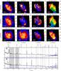
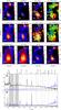
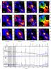
As mentioned above, the maps of the emission lines were constructed by fitting a single Gaussian profile to the spectra. Figure 1 shows, for the subsample of 10 LIRGs, the Brγ and H2 1−0S(1) emission and equivalent width maps, together with the velocity dispersion and radial velocity ones. The figures also include emission maps of the HeI at 2.059 μm and, for those objects observed in the H band, [FeII] line emission maps at 1.644 μm. We have also constructed a K band map from the SINFONI data by integrating the flux along the response curve of the 2MASS K-band filter, to compare with archival HST images when available. Figure 2 shows the maps of the subsample of 7 ULIRGs but with the Paα emission line instead of Brγ. All the line emission maps are shown in arbitrary units on a logarithmic scale to maximise the contrast between the bright and diffuse regions and are oriented following the standard criterium that situates the north up and the east to the left2.
The radial velocity maps are scaled to the velocity measured at the brightest spaxel in the K band image. This spaxel is marked with a cross in all the maps and usually coincides with the nucleus of the galaxy or with one of them for the interacting systems. The measured systemic radial velocities are similar to the NED published values within less than ~1%. Although the main nucleus of NGC 3256 was observed in the H band, the reference spaxel corresponds to its southern nucleus, which is highly extinguished (Kotilainen et al. 1996; Alonso-Herrero et al. 2006; Díaz-Santos et al. 2008), since the main one was not observed in the K band (see Fig. 1c). The values of the reference radial velocities are shown in Table 4.
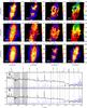 |
Fig. 1a NGC 2369. Top and middle panels are SINFONI observed maps (not corrected from extinction) of the lines Brγ λ2.166 μm, and H2 1−0S(1)λ 2.122 μm. From left to right: flux, equivalent width, velocity dispersion and velocity. Lower panel shows, from left to right, the K band emission from our SINFONI data, HST/NICMOS F160W continuum image from the archive, HeIλ2.059 μm, and [FeII]λ1.644 μm emission maps. The brightest spaxel of the SINFONI K band is marked with a cross. The apertures used to extract the spectra at the bottom of the figure are drawn as white squares and labelled accordingly. At the bottom, the two rest-frame spectra extracted from apertures “A” and “B” are in black. The most relevant spectral features are labelled at the top and marked with a dotted line. The sky spectrum is overplotted as a dashed blue line, and the wavelength ranges of the water vapour atmospheric absorptions are marked in light grey. |
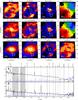 |
Fig. 1d As Fig. 1a but for ESO 320-G030. |
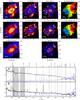 |
Fig. 1e As Fig. 1a but for IRASF 12115-4656. |
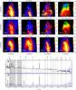 |
Fig. 1g As Fig. 1a but for IRASF 17138-1017. |
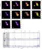 |
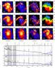
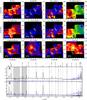
Fig. 2a IRAS 06206-6315. Top and middle panels are SINFONI observed maps (not corrected from extinction) of the lines Paα λ1.876 μm, and H2 1−0S(1)λ 2.122 μm. From left to right: flux, equivalent width, velocity dispersion, and velocity. Lower panel shows, from left to right, the K band emission from our SINFONI data, HST continuum image from the archive, and HeIλ2.059 μm (when available). The brightest spaxel of the SINFONI K band is marked with a cross. The apertures used to extract the spectra at the bottom of the figure are drawn as white squares and labelled accordingly. At the bottom, the two rest-frame spectra extracted from apertures “A” and “B” in black. The most relevant spectral features are labelled at the top and marked with a dotted line. The sky spectrum is overplotted as a dashed blue line, and the wavelength ranges of the water vapour atmospheric absorptions are marked in light grey. |
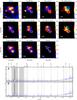 |
Fig. 2b As Fig. 2a but for IRAS 12112+0305. |
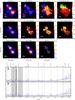 |
Fig. 2c As Fig. 2a but for IRAS 14348-1447. |
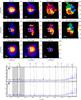 |
Fig. 2d As Fig. 2a but for IRAS 17208-0014. |
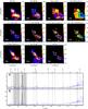 |
Fig. 2e As Fig. 2a but for IRAS 21130-4446. |
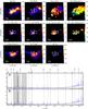 |
Fig. 2f As Fig. 2a but for IRAS 22491-1808. |
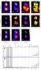 |
Fig. 2g As Fig. 2a but for IRAS 23128-5919. |
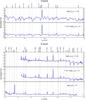 |
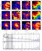
Fig. 3 H- and K-band stacked spectra of the SINFONI sample, divided into three subsets with log(LIR/L⊙) < 11.35, 11.35 ≤ log(LIR/L⊙) < 12, and log(LIR/L⊙) ≥ 12. The spectra are normalised to a linear fit of the continuum measured within the intervals [1.600, 1.610] μm and [1.690, 1.700] μm for the H band and [2.080, 2.115] μm and [2.172, 2.204] μm for the K band. From top to bottom, H-band and K-band spectra of the different subsets by increasing LIR. The spectra are available in electronic form at the CDS. |
Besides the spectral maps, Figs. 1 and 2 show, for illustrative purposes, the integrated spectra in the K band of two regions of the FoV. The apertures used to extract the spectra are drawn on the maps and are labelled with the letters “A” and “B”. Aperture “A” is centred on the brightest spaxel of the K band image, which usually corresponds to the nucleus of the galaxy. On the other hand, aperture “B” is centred in regions of interest that differ from object to object. In the LIRG subsample, it covers the brightest region in the Brγ equivalent width map. The same criterion is used for the ULIRG subsample, except in those objects with two distinct nuclei, where aperture “B” covers the secondary nucleus.
The spectra are normalised to the continuum, measured between 2.080 μm and 2.115 μm and between 2.172 μm and 2.204 μm. We also stacked the spectra of one of our sky cubes into a single spectrum and plotted it to illustrate the typical sky emission. This is useful for identifying the residuals from sky lines that are the result of the sky subtraction during the data reduction. Besides the OH sky lines, some of the K-band spectra show the residuals from the atmospheric absorption of water vapour. These features are easily traced along the wavelength ranges [1.991−2.035] μm and [2.045−2.080] μm, and are marked in grey in Figs. 1 and 2.
3.6. Generation of the stacked spectra for the LIRG and ULIRG subsamples
Figure 3 shows the stacked spectra of three different subsets of the sample defined according to the LIR range. As discussed in Rosales-Ortega et al. (2012), there are different techniques for optimising the S/N within IFS data. We have adopted a flux-based criterium to exclude those spaxels with low surface brightness that may contribute to increase the noise of the resulting spectra. For each object, we considered the continuum images for each band and ordered the spaxels by decreasing flux. We then selected a set of spectra from those spaxels that contain at least the ≳90% of the total continuum flux. By assuming this criterium, we assure that typically between the ~85−95% of the flux in the lines is also taken into account.
Before the stacking, every individual spectrum is de-rotated, i.e. shifted to the same rest frame. This procedure decorrelates the noise due to imperfect sky subtraction, since the residuals are no longer aligned in the spectral axis, and prevents the smearing of the lines due to the stacking along wide apertures. To derotate the spectra, we focussed on the [FeII] line for the H band and on Brγ (Paα for the ULIRG subset) and the H2 1−0S(1) line for the K band, since the relative shifts in the spectral axis could be different for each phase of the gas. For the ULIRG subset, we have only considered the Paα line, since the H2 1−0S(1) line is not bright enough in all the spaxels where the spectra are extracted. For the K band spectra of the LIRG subsample, we measured the difference between the relative shifts obtained for the Brγ and H2 lines, to assure that no artificial broadening is introduced if only one phase is considered as reference for the whole spectra. Given that only less than ~10% of the spaxels have more than one spectral pixel of difference between the relative shifts measured with both emission lines, we considered that the effect in the width of the lines is negligible so we have adopted the Brγ line as reference for the whole LIRG subset.
After the derotation procedure, every spectrum of each object is normalised to a linear fit of the continuum, measured within the intervals [1.600, 1.610] μm and [1.690, 1.700] μm for the H-band and [2.080, 2.115] μm and [2.172, 2.204] μm for the K-band, and stacked in one single spectrum per object. Finally, the spectra of each galaxy in each luminosity bin are rebinned, stacked, and convolved to a resolution of 10 Å (FWHM) to achieve a homogeneous resolution. The spectra of the different luminosity bins are available at the CDS.
3.7. Gas emission and line fluxes
We extracted the spectra of different regions of interest for all the galaxies of the sample, which comprise the nucleus (identified as the K-band continuum peak), the integrated spectrum over the FoV, and the peak of emission of Brγ (Paα for the ULIRGs subsample), H2 1−0S(1), and [FeII]. For every region, we integrated the spectra within apertures of 400 × 400 pc for the LIRGs and 2 × 2 kpc for ULIRGs, and measured the flux of the Brγ, H2 1−0S(1), and [FeII] lines for all the LIRGs of the sample and the Paα and H2 1−0S(1) line flux for the ULIRGs subsample. Although the study of the ionised gas is focussed on the Paα line in the ULIRG subset, we have also made measurements of the Brγ line to directly compare with the results obtained for the LIRGs.
To obtain the line fluxes over the FoV, we only took the brightest spaxels in the H and K-band images (for the [FeII] and Brγ Paα and H2 1−0S(1) respectively) into account, to include ≳90% of the total flux in each image. This ensures that only those spaxels with the highest S/N are included in the spectra, and removes all those with a low surface brightness that contributes significantly to increasing the noise and the sky residuals in the spectra.
The line fitting is performed following the same procedure as in the spectral maps, by fitting a single Gaussian model to the line profile. To estimate the errors of the line fluxes, we implemented a Monte Carlo method. We measured the noise of the spectra as the rms of the residuals after subtracting the Gaussian profile. Taking this value of the noise into account, we constructed a total of N = 1000 simulated spectra whose lines are again fitted. The error of the measurements is obtained as the standard deviation of the fluxes of each line. The advantage of this kind of method is that the errors calculated not only consider the photon noise but also the uncertainties due to an improper line fitting or continuum level estimation.
The values of the line fluxes for the different regions in the sample of galaxies are shown in Table 5. Besides the gas emission, we also measured the equivalent width of the CO (2−0) band at 2.293 μm (WCO) using the definition of Förster Schreiber (2000). This stellar feature is detected in all the galaxies of the LIRG subsample and in two ULIRGs (IRAS 17208-0014 and IRAS 23128-5919), since it lays out of our spectral coverage for the rest of the ULIRGs.
3.8. Stellar absorption features
Although the study of the stellar populations and of their kinematics, derived from the CO absorption lines, will be addressed in a forthcoming paper (Azzollini et al., in prep.), we have included measurements of the equivalent width of the first CO absorption band (see Table 5) obtained using the penalised PiXel-Fitting (pPXF) software (Cappellari & Emsellem 2004) to fit a library of stellar templates to our data. We made use of the Near-IR Library of Spectral templates of the Gemini Observatory (Winge et al. 2009), which covers the wavelength range of 2.15−2.43 μm with a spectral resolution of 1 Å pixel-1. The library contains a total of 23 late-type stars, from F7III to M3III, and was previously convolved to our SINFONI resolution.
Brγ, H2 1−0S(1), and [FeII] integrated observed fluxes and CO (2-0) equivalent widths of the LIRG subsample.
Paα and H2 1−0S(1) integrated observed fluxes and CO (2-0) equivalent widths of the ULIRGs subsample.
4. Overview of the data
The wide spectral coverage of the SINFONI data allows us to study in detail a large number of spectral features that trace different phases of the interstellar medium and the stellar population (Bedregal et al. 2009). In this work we focus on the gas emission in LIRGs and ULIRGs by studying the brightest lines in the H and K bands, i.e. [FeII] at 1.644 μm, Paα at 1.876 μm, HeI at 2.059 μm, H2 1−0S(1) at 2.122 μm and Brγ at 2.166 μm. The maps of these spectral features together with the K-band spectra of the nucleus (identified as the K-band peak), and of the brightest Brγ (or Paα for ULIRGs) region are shown in Figs. 1 and 2 for the sample of LIRGs and ULIRGs, respectively.
In the present section, we briefly describe the different physical mechanisms and processes that create the emission lines and stellar features observed in our data. The detailed study of these mechanisms are beyond the scope of the present work, but some of them will be addressed in the forthcoming papers of these series.
4.1. Hydrogen lines and 2D extinction maps
The overall structure of the ionised gas, mostly associated with recent star formation, is traced by the hydrogen recombination lines Paα for ULIRGs and Brγ for LIRGs. Although Brγ is also observed in the ULIRGs subsample, for this group we focus the study of the ionised gas on the Paα emission, since its brightness allows better measurements. The Brδ line at 1.945 μm is also observed in all the galaxies of the sample; however, for the LIRG subsample, it lies in a spectral region where the atmospheric transmission is not optimal and, for the ULIRG subset, it is too weak to be mapped.
It is well known that the bulk of luminosity produced in local (U)LIRGs is due to the large amount of dust that hides a large fraction of their star formation and nuclear activity (see Alonso-Herrero et al. 2006; García-Marín et al. 2009a, and references therein). This dust is responsible for the absorption of UV photons that are then re-emitted at FIR and submillimetre wavelengths. A detailed 2D quantitative study of the internal extinction could be performed by using the Brδ/Brγ ratios in LIRGs and Brγ/Paα in ULIRGs. This study of the objects in the sample will be presented in the next paper of this series (Paper II, Piqueras López et al. 2012a, in prep.).
The detailed characterisation of the extinction is essential to accurate measurement of the SFR in these dusty environments. This treatment of the extinction allows us to obtain maps of the SFR surface density that are corrected for extinction on a spaxel-by-spaxel basis. The analysis of the SFR in the objects of the sample, based on the Brγ and Paα maps presented in this work, will be addressed in Piqueras-López et al. (2012b, in prep.).
4.2. Emission lines and star formation
The hydrogen recombination lines have been widely used as a primary indicator of recent star-formation activity, where UV photons from massive OB stars keep the gas in an ionised state. The measurements of the Brγ equivalent width (EW), in combination with the stellar population synthesis models, such as STARBURST99 (Leitherer et al. 1999) or Claudia Maraston’s models (Maraston 1998, 2005), could be used to constrain the age of the youngest stellar population. The HeI emission is also usually associated to star-forming regions, and used as a tracer of the youngest OB stars, given its high ionisation potential of 24.6 eV. This emission may depend on different factors, such us density, temperature, dust content, and He/H relative abundance and ionisation fractions.
The [FeII] emission is usually associated with regions where the gas is partially ionised by X-rays or shocks (Mouri et al. 2000). Shocks from supernovae cause efficient grain destruction that releases the iron atoms contained in the dust. The atoms are then singly ionised by the interstellar radiation field and excited in the extended post-shock region by free electron collision on timescales of ~104 yr. The [FeII] lines at 1.257 μm and 1.644 μm are widely used to estimate the supernova rate in starbursts (Colina 1993; Alonso-Herrero et al. 2003; Labrie & Pritchet 2006; Rosenberg et al. 2012, and references therein), whereas the EW[FeII] could also be used, in combination with the EWBrγ, to constrain the age of the stellar populations in the synthesis models.
4.3. H2 lines and excitation mechanisms
The H2 1−0S(1) line is used to trace the warm molecular gas, since it is the brightest H2 emission line in the K band and it is well detected in all the objects with sufficient S/N. Furthermore, the presence of several roto-vibrational transitions of the molecular hydrogen within the K band allows studying the excitation mechanisms of the H2: fluorescence due to the excitation by UV photons from AGB stars in PDRs (photon-dominated regions), thermal processes like collisional excitation by SN fast shocks, or X-rays (van der Werf 2001; Davies et al. 2003, 2005). The determination of the H2 excitation mechanisms in general requires measurements of several lines, usually weak lines, since the different processes mentioned may rise to similar intense and thermalised 1−0 emissions.
Based on the relative fluxes of the transitions to the brightest H2 1−0S(1) line, we could obtain population diagrams of the emitting regions. In these diagrams, the population of each level in an ideal thermalized PDR could be determined as a function of the excitation temperature. The presence of non-thermal processes like UV fluorescence is translated to an overpopulation of the upper levels and a deviation from the ideal thermalised model. However, the way these levels are overpopulated due to non-thermal processes is complex, and might depend on several parameters like density or the intensity of the illuminating UV field (Davies et al. 2003, 2005; Ferland et al. 2008, and references therein). The detailed study of the excitation mechanisms of the molecular hydrogen will be addressed in a future paper of this series (Piqueras López et al. 2012c, in prep.).
4.4. Coronal lines as AGN tracers
The [SiVI] at 1.963 μm and [CaVIII] at 2.321 μm coronal lines are the main AGN tracers within the K-band. However, the [CaVIII] line is too faint (typically ×4 fainter than [SiVI], Rodríguez-Ardila et al. 2011) and to close to CO (3−1) to be measured easily. Given the high ionisation potential of 167 eV for [SiVI] and 128 eV for [CaVIII], the outskirts of the broad-line region and extended narrow-line regions have been proposed as possible locations for the formation of these lines in AGNs. Although which mechanism is responsible for the emission remains unclear, there are two main processes proposed: photoionisation due to the central source and shocks due to high-velocity clouds and the NLR gas (see Rodríguez-Ardila et al. 2011, and references therein).
4.5. Line ratios
The interpretation of the H2 1−0S(1)/Brγ ratio is sometimes not straightforward since H2 could be excited by both thermal and radiative processes, in contrast to the [FeII] emission that is predominantly powered by thermal mechanisms. This ratio is in principle not biased by extinction, and starburst galaxies and HII regions empirically exhibit lower H2/Brγ ratios, whereas Seyfert galaxies and LINERs show higher values (0.6 ≲ H2 1−0S(1)/Brγ ≲ 2.0, Dale et al. 2004; Rodríguez-Ardila et al. 2005; Riffel et al. 2010; Valencia-S et al. 2012).
In combination with the Brγ emission that traces the photoionised regions, the [FeII]/Brγ ratio allows us to distinguish regions where the gas is ionised by star formation activity where the [FeII] is expected to be weak (Mouri et al. 2000), from zones where the gas is partially ionised by shocks (Alonso-Herrero et al. 1997). Since [FeII] is not expected in HII regions where iron would be in higher ionisation states, we could trace different ionisation mechanisms and efficiencies by using the [FeII]/Brγ ratio, and probe the excitation mechanisms that produce the [FeII] line in those regions where the emission has stellar origin. In addition, the [FeII]/Brγ ratio depends on the grain depletion, and a high depletion of iron would reduce the number of atoms available in the interstellar medium, hence reduce the line ratio (Alonso-Herrero et al. 1997).
Although the HeI line could be used as a primary indicator of stellar effective temperature, interpreting the emission and the HeI/Brγ ratio without a detailed photoionisation model is still controversial (Doherty et al. 1995; Lumsden et al. 2001, 2003). In addition, the HeI transition is also influenced by collisional excitation, and a full photoionisation treatment is not enough to predict the line emission (Shields 1993).
4.6. Absorption lines and stellar populations
Besides the emission lines, there are different absorption features that lie within the K band, such as the NaI doublet at 2.206 μm and 2.209 μm, the CaI doublet at 2.263 μm, and 2.266 μm and the CO absorption bands CO (2−0) at 2.293 μm, CO (3−1) at 2.323 μm or CO (4−2) at 2.354 μm. The absorption features, such as the CO bands and the NaI doublet, are typical of K and later stellar types, and they also trace red giant and supergiant populations. Given the limited S/N of the NaI doublet, it is not possible to map the absorption with the present data, but it could be suitable for integrated analysis. On the other hand, the CO (2−0) band can be used to spatially sample the stellar component of all the LIRGs of the sample and in two of the ULIRGs. Both EWCO and EWNaI could be used in combination with the stellar population synthesis models to constrain the age of the stellar populations (see Bedregal et al. 2009).
5. Results and discussion
Most of the LIRGs of the sample are spiral galaxies with some different levels of interaction, ranging from isolated galaxies as ESO 320-G030 to close interacting systems as IC 4687+IC 4686 or mergers like NGC 3256 (Lípari et al. 2000), and to objects that show long tidal tails several kiloparsecs away from its nucleus (e. g. NGC 7130, Fig. 1i). The emission from ionised and molecular hydrogen has different morphologies in many galaxies of the LIRGs subsample. The ULIRG subsample contains mainly interacting systems in an ongoing merging process with two well-differentiated nuclei. The Paα emission extends over several kiloparsecs with bright condensations not observed in the continuum maps. The molecular hydrogen emission, on the other hand, is rather compact (≲2−3 kpc) and is associated with the nuclei of the systems. An individual description of the more relevant features of the gas emission morphology for each galaxy can be found in Appendix A. We now discuss each gas phase and the stellar component separately.
5.1. Ionised gas
The dynamical structures as spiral arms are clearly delineated on the ionised gas maps traced by the Brγ (LIRGs) and Paα (ULIRGs) lines. The observed ionised gas emission in LIRGs is dominated by high surface brightness clumps associated with extranuclear star-forming regions located in circumnuclear rings or spiral arms at radial distances of several hundred parses. The nuclei are also detected as bright Brγ sources in several galaxies but represent the maximum emission peak in only a small fraction (~33%) of LIRGs. These results are in excellent agreement with those derived from the Paα emission in Alonso-Herrero et al. (2006) using HST NICMOS images for all the objects of our LIRG sample, with the exception of IRASF 12115-4656, which was not included in their sample. On the other hand, the main nucleus is the brightest Paα emission peak in the majority (~71%) of ULIRGs, also showing emission peaks along the tidal tails, secondary nucleus, or in extranuclear regions at distances of 2−4 kpc from their centre. However, since ULIRGs in our sample are about four to five times more distant than our LIRGs, the typical angular resolution of our SINFONI maps for ULIRGs covers sizes of about 1.5 kpc, and therefore the Paα peak emission detected in the nuclei could still be due to circumnuclear star-forming regions, as in LIRGs.
The surface density and total luminosity distributions of the Brγ (and Paα for the ULIRG subsample) are presented in Figs. 7 and 8. On average, the observed (i.e. uncorrected for internal extinction) luminosities of the Brγ brightest emitting region are ~1.2 × 10⁵ L⊙ for LIRGs and ~2.3 × 10⁶ L⊙ for ULIRGs, accounting for about ~10% and ~43% of the integrated Brγ luminosity, respectively. There is a factor ~20 difference in luminosity between LIRGs and ULIRGs. Although the ULIRGs are intrinsically more luminous, this difference is also due to a distance effect since the angular aperture used to obtain the luminosities covers for ULIRGs an area 25 times larger than for LIRGs. For the ULIRG subset, we have also measured peak Paα luminosities of the order of 4.5 × 10⁷ L⊙, in agreement with the expected value derived from Brγ luminosities assuming case B recombination ratios and no extinction.
The observed Brγ surface luminosity densities of the Brγ (and Paα) brightest emitting regions are ~0.7 L⊙ pc-2 and ~0.6 L⊙ pc-2, on average, for LIRGs and ULIRGs, respectively, whereas the Paα surface density for the ULIRG subset is ~6 L⊙ pc-2. Figure 8 shows that the distributions of the Brγ surface luminosity density for the different luminosity bins are very similar for the Brγ (and Paα) peak and the nucleus of the objects, and range between ~0.1 L⊙ pc-2 and ~3 L⊙ pc-2.
As shown in Fig. 7, the luminosity of
Brγ ranges
from ~1.7×10⁴ L⊙
to ~5.1×10⁶ L⊙ in the nuclear regions of
LIRGs, and the Paα emission reaches up
to ~5.0×10⁷ L⊙ in ULIRGs. Assuming the
standard star formation rate to Hα luminosity ratio given by the
expression (Kennicutt 1998),
 an estimate of the SFR surface densities,
uncorrected for internal reddening, can be directly obtained from the previous expression
if the Hα to Paα and Brγ recombination
factors are taken into account:
an estimate of the SFR surface densities,
uncorrected for internal reddening, can be directly obtained from the previous expression
if the Hα to Paα and Brγ recombination
factors are taken into account: 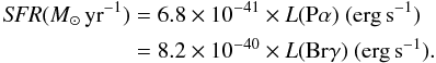 For LIRGs, the mean SFR surface densities
integrated over areas of several kpc2, range between 0.4 and
0.9 M⊙ yr-1 kpc-2 with peaks of about
2−2.5 M⊙ yr-1 kpc-2 in smaller regions
(0.16 kpc2) associated with the nucleus or the brightest Brγ
region. For ULIRGs, the corresponding values are similar, ~0.4 for the integrated
emission and ~2 M⊙ yr-1 kpc-2 for
peak emission. However, since ULIRGs are at distances further away than LIRGs, the sizes
of the overall ionised regions and brightest emission peaks covered by the SINFONI data
are greater than those in LIRGs, and they correspond to 100−200 kpc2
and 4 kpc2, respectively.
For LIRGs, the mean SFR surface densities
integrated over areas of several kpc2, range between 0.4 and
0.9 M⊙ yr-1 kpc-2 with peaks of about
2−2.5 M⊙ yr-1 kpc-2 in smaller regions
(0.16 kpc2) associated with the nucleus or the brightest Brγ
region. For ULIRGs, the corresponding values are similar, ~0.4 for the integrated
emission and ~2 M⊙ yr-1 kpc-2 for
peak emission. However, since ULIRGs are at distances further away than LIRGs, the sizes
of the overall ionised regions and brightest emission peaks covered by the SINFONI data
are greater than those in LIRGs, and they correspond to 100−200 kpc2
and 4 kpc2, respectively.
We estimated the extinction effects by comparing the observed Brγ/Brδ and Brγ/Paα ratios (for LIRGs and ULIRGs, respectively) with the theoretical ones derived from a case B recombination. We measured AV values that range from ~2−3 mag up to ~10−12 mag in the nuclei of the objects (Piqueras López et al. 2012a, in prep.). This is translated to extinction values from ~0.3 mag to ~1.0 mag at Brγ wavelengths, and from ~0.4 mag to ~1.6 mag at Paα, and indicates that the internal extinction in these objects still plays a role at these wavelengths. These values are similar to those obtained by Alonso-Herrero et al. (2006) from the nuclear emission in LIRGs. From the detailed 2D study of the internal extinction that will be presented in Paper II, we estimated the median visual extinction for each luminosity subsamples of LIRGs and ULIRGs. These values are AV,LIRGs = 6.5 mag and AV,ULIRGs = 7.1 mag, that correspond to ABrγ = 0.6 mag and APaα = 1.0 mag respectively.
Considering the median extinction values presented above, the Brγ and Paα luminosities, hence the SFR surface densities, are underestimated approximately by a factor ×1.7 in LIRGs and ×2.5 in ULIRGs. However, on scales of a few kpc or less, the distribution of dust in LIRGs and ULIRGs is not uniform, and it shows a patchy structure that includes almost transparent regions and very obscured ones (see García-Marín et al. 2009a; Paper II). This non-uniform distribution of the dust implies that the correction from the extinction depends on the sampling scale, so that the correction to the SFR would depend on the scales where the Brγ (Paα) is sampled. For further discussion of the extinction and the implications of the sampling scale in its measurements, please see Piqueras López et al. (2012a, in prep.).
A detailed analysis of SFR surface densities based on the Brγ, Paα, and Hα emission lines will be presented elsewhere (Piqueras López et al. 2012b, in prep.).
5.2. Warm molecular gas
The H2 emission is associated with the nuclear regions of the objects, either to the main nucleus or to the secondary in the interacting systems. In some cases, its maximum does not coincide with the Brγ peak, although in all the LIRGs and ~71% of the ULIRGs it coincides with the main nucleus, identified as the brightest region in the K-band image. The typical H2 1−0S(1) luminosity of the nuclei ranges from ~1.3×10⁵ L⊙ for the LIRG subsample up to ~4.6×10⁶ L⊙ for the ULIRGs, and accounts for ~13% and ~41% of the total luminosity measured in the entire FoV. The H2 luminosity observed in the nucleus and in the Brγ (Paα) peak in both LIRGs and ULIRGs is very similar to the Brγ luminosity. The range of observed luminosity in the nuclei spans from ~4.2×10⁴ L⊙ to ~6.8×10⁶ L⊙, and is also very similar to the distribution observed for the Brγ emission. Since the H2 (1−0)/Brγ ratio is close to one (range of 0.4 to 1.4, see Fig. 6), the surface brightness values derived for the H2 emission are similar to those obtained for Brγ (see Fig. 8).
5.3. Partially ionised gas
The [FeII] maps reveal that the emission roughly traces the same structures as the Brγ line, although the emission peaks are not spatially coincident in some of the objects, and the [FeII] seems to be more extended and diffuse. In ~55% of the LIRGs, the peak of the [FeII] emission is measured in the nucleus, with typical luminosities of ~1.2×10⁵ L⊙ on scales of ~0.16 kpc2. The nuclear emission accounts on average for ~16% of the total observed luminosity. The differences in the morphology between the ionised and partially ionised gas could be understood in terms of the local distribution of the different stellar populations: although both lines trace young star-forming regions, the Brγ emission is enhanced by the youngest population of OB stars of ≲6 Myr, whereas the [FeII] is mainly associated with the supernova explosions of more evolved stellar populations of ~7.5 Myr (see STARBURST99 models, Leitherer et al. 1999).
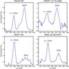 |
Fig. 4 H2 1−0S(3) and [SiVI] normalised flux profiles of the brightest spaxel in [SiVI] for the four objects where the coronal line is detected. |
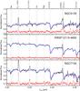 |
Fig. 5 Zoom around the region containing the stellar absorption features and the coronal line [CaVIII] at 2.321 μm for three of the objects where coronal emission is detected. Spectra correspond to the brightest spaxel in [SiVI] (see Fig. 4). The pPXF fitting of the stellar absorptions is plotted in blue, and the residuals from the fitting are shown as a red dotted line. |
5.4. Coronal line emission
The [SiVI] coronal line at 1.963 μm (see Fig. 4) is detected in two LIRGs (NGC 5135 and IRASF 12115-4656) and in one ULIRG (IRAS 23128-5919), with a tentative detection in another LIRG (NGC 7130). The [SiVI] line has a high ionisation potential (167 eV) and it is associated with Seyfert activity where the gas is ionised outside the broad line region of the AGN (Bedregal et al. 2009). The [SiVI] emission is usually rather compact, concentrated around the unresolved nucleus and extending up to a few tens or a few hundred parsecs in some Seyferts (Prieto et al. 2005; Rodríguez-Ardila et al. 2006). While in galaxies like IRASF 12115-4656 and IRAS 23128-5919 the emission is unresolved (i.e. sizes less than ~150 pc and ~550 pc, respectively), a relevant exception is NGC 5135, which presents a cone of emission centred on the AGN and extending ~600 pc (~2 arcsec) from the nucleus, as discussed in Bedregal et al. (2009). The line profiles for the four galaxies are given in Fig. 4.
As shown in Fig. 5, the [CaVIII] coronal line at 2.321 μm is also detected in three of these objects, NGC 5135, IRASF 12115-4656 and tentatively in NGC 7130. Although the [CaVIII] line lays also within the rest-frame spectral coverage of IRAS 23128-5919, the S/N in this region of the spectra is very low, so was not included in the figure.
5.5. Characteristics of the near-IR stacked spectra of LIRGs and ULIRGs
To obtain representative spectra of LIRGs and ULIRGs, we divided the sample into three subsamples according to their total infrared luminosity (see Sect. 3.6), i.e. low luminosity bin, log(LIR/L⊙) < 11.35; intermediate, 11.35 ≤ log(LIR/L⊙) < 12; and high, the ULIRGs subsample, log(LIR/L⊙) ≥ 12. The average luminosities for each bin are log(LIR/L⊙) = 11.23, log(LIR/L⊙) = 11.48, and log(LIR/L⊙) = 12.29. Each luminosity bin contains a similar number of objects in each subsample, six, four, and seven, respectively. The stacked spectra for each luminosity bin are presented in Fig. 3.
Brγ, H2 1−0S(1), and [FeII] velocity dispersion values of the LIRGs subsample.
Paα and H2 1−0S(1) velocity dispersion values of the ULIRGs subsample
Brγ (and Paα) average luminosities and surface brightness for the U/LIRGs according to their LIR.
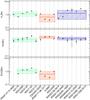 |
Fig. 6 H2/Brγ (top), HeI/Brγ (centre), and [FeII]/Brγ (bottom) line ratios of the galaxies of the sample, ordered by increasing LIR. The values are measured in the integrated spectra. The weighted mean of each luminosity bin (low, log(LIR/L⊙) < 11.35; intermediate, 11.35 ≤ log(LIR/L⊙) < 12 and high, log(LIR/L⊙) ≥ 12) is plotted as a thick line, whereas the box represents the standard deviation of the values. Since all the ULIRGs and one LIRG were not observed in the H-band, [FeII]/Brγ data are presented for only nine LIRGs. |
The H-band spectrum of LIRGs is dominated by the stellar continuum, with pronounced absorption features from water vapour and CO. The main emission feature is the [FeII] line at 1.644 μm, while the faint high-order hydrogen Brackett lines (Br10 to Br14) are also present. The K-band spectra show various stellar absorption features like the faint NaI, CaI, MgI, lines and the strong CO bands. The emission line spectra contain the hydrogen (Brγ and Brδ) and He recombination lines, as well as a series of the H2 lines covering different transitions. While the [SiVI] coronal line is detected in some LIRGs and ULIRGs, it is a weak line and thus not visible in the stacked spectra at any luminosity. The average luminosity and surface brightness of the Brγ and Paα emission for each bin is shown in Table 7.
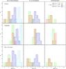 |
Fig. 7 Luminosity distribution of the Brγ, H2 1−0S(1), and [FeII] emission. From top to bottom, the histograms show the distribution of the total luminosity in solar units of the lines measured in the nucleus (defined by aperture “A” in Figs. 1 and 2), the integrated FoV, and the peak of the Brγ (Paα) emission. For the distributions of the ionised gas (first column), we have also included the Paα emission in light blue for the ULIRGs. Note: Brγ (Paα) peak coincides with the nucleus in ~33% of the LIRGs and in the ~71% of the ULIRGs. |
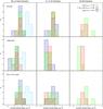 |
Fig. 8 Surface density distribution of the Brγ, H2 1−0S(1), and [FeII] emission. From top to bottom, the histograms show the distribution of the surface density in solar units per unit of area (pc2) of the lines measured in the nucleus (defined by aperture “A” in Figs. 1 and 2), the integrated FoV, and the peak of the Brγ (Paα) emission. For the distributions of the ionised gas (first column), we have also included the Paα emission in light blue for the ULIRGs. The Brγ (Paα) peak coincides with the nucleus in ~33% of the LIRGs and in the ~71% of the ULIRGs. |
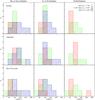 |
Fig. 9 Distributions of the velocity dispersion of the ionised gas (Brγ for LIRGs Paα for ULIRGs), H2 1−0S(1), and [FeII] emission. From top to bottom, the histograms show the distributions of the velocity dispersion measured in the nucleus (defined by aperture “A” in Figs. 1 and 2), the integrated FoV, and the peak of the Brγ (Paα) emission. The Brγ (Paα) peak coincides with the nucleus in ~33% of the LIRGs and in the ~71% of the ULIRGs. |
Considering only the brightest emission lines that trace different phases of the gas and/or excitation conditions, there appears to be some small differences (~1 σ) in their ratios with the LIR(see Fig. 6 for the H2 1−0S(1)/Brγ, HeI/Brγ, and [FeII]/Brγ line ratios measured for the different luminosity bins). The HeI/Brγ ratio is slightly higher (× 1.3) in intermediate and high luminosity galaxies than in low luminosity objects. A plausible interpretation could be that young and massive stars in low luminosity LIRGs represent a lower fraction than in more luminous infrared galaxies. Whether this could be caused by age effects or by lower IMF upper mass limits remains to be investigated in more detail. Some differences are also identified in the H2 1−0S(1)/Brγ line ratio. While this ratio is close to unity for low luminosity LIRGs, it drops to about 0.6 for intermediate luminosity LIRGs, and increases up to about 1.3 for the most luminous galaxies. However, given the large dispersion of the values for the individual objects, and the low number of galaxies in each bin, we could not draw any significant conclusion about these differences. While low H2 1−0S(1)/Brγ values appear to be characteristic of starbursts (H2 1−0S(1)/Brγ ≲ 0.6), classical Seyfert 1 and 2 galaxies also display a range of values (Rodríguez-Ardila et al. 2004, 2005; Riffel et al. 2010) that are compatible with those measured in our sample.
The [FeII]/Brγ ratio also shows values compatible with those observed in starbursts, although higher values would have been expected for Seyfert galaxies, such as NGC 5135 and NGC 7130 (Rodríguez-Ardila et al. 2004; Riffel et al. 2010; Valencia-S et al. 2012). These galaxies show the highest values of the [FeII]/Brγ ratio of the whole sample, close to ~2.0, and are similar to values reported for other Seyfert 2 galaxies (Blietz et al. 1994). These differences could be related to the different apertures used to extract the integrated values of the ratios. Even more, the reported ratios are observed values (not corrected for extinction). Although the H2 1−0S(1)/Brγ ratio is almost unaffected by extinction, the [FeII]/Brγ ratio could be affected by obscuration, so that an accurate study of the extinction is needed to confirm or dismiss these discrepancies between both ratios.
Based on our current survey, no evidence of relevant differences in the emission line spectra of LIRGs and ULIRGs appear as a function of LIR. A larger sample would be required to confirm the differences in the emission line ratios presented here, since they are still compatible within the uncertainties. The full two-dimensional study of the line ratios and the ionisation and excitation mechanisms of the gas will be addressed in a future paper of the series (Piqueras López et al., in prep.), since its detailed analysis is beyond the scope of the present work.
5.6. Stellar component
In Table 5, we have included the EW of the first absorption band of the CO at 2.293 μm. In most of the objects, the values correspond to the Brγ (Paα) peak and nucleus, which are the regions with enough S/N in the continuum to detect the band. The nuclear values of the LIRGs are 7.1 Å ≤ EWCO ≤ 12.3 Å, with typical uncertainties of ~10% and an average of 10.6 Å whereas the values measured at the Brγ (Paα) peak cover the range 8.3 Å ≤ EWCO ≤ 12.2 Å, with the same uncertainties and a mean value of 10.7 Å. According to the stellar population synthesis models like STARBURST99 (Leitherer et al. 1999), these values of the EW correspond to stellar populations older than log T(yr) ~ 6.8 and up to log T(yr) ~ 8.2 or more, depending on whether we consider a instantaneous burst or a continuum star-formation activity. The detailed study of the 2D distribution of the stellar populations using the CO stellar absorption, the H, and He emission lines will be addressed in forthcoming papers.
5.7. Kinematics of the gas
Besides the general morphology and luminosities of the different emission lines, their 2D kinematics (velocity field and velocity dispersion maps) are also presented (Figs. 1 and 2). We obtained the velocity dispersion of the different regions of interest described above, i.e. nucleus, the emission peaks of the Brγ (Paα), H2 1−0S(1) and [FeII] lines, and the entire FoV. The values of the velocity dispersion, corrected for the instrumental broadening, are shown in Table 6. The errors are obtained following the same Monte Carlo method implemented to estimate the flux error. Figure 9 shows the distributions of the velocity dispersion obtained from the values of Table 6. The distributions show that there is no clear relationship between the LIR of the objects and the velocity dispersion of the different regions, although the highest values of velocity dispersion tend to come from high-luminosity objects where measurements come from scales ×4−5 larger, so could be affected by beam smearing.
The average velocity dispersion of the Brγ and H2 1−0S(1) lines in the LIRGs is ~90 km s-1, whereas the measured average values for the ULIRG subsample are ~140 km s-1 and ~120 km s-1, respectively. The higher velocity dispersion measured in the ULIRG subset can be explained mainly as a distance effect: the contribution from the unresolved velocity field to the width of the line is larger since the physical scales are also larger. We estimated this effect by extracting several spectra over apertures of increasing radius and measuring the width of the Brγ and H2 1−0S(1) lines in one of the objects of the LIRG subset. We used NGC 3110 since the Brγ and H2 emitting gas is extended and well sampled in almost the entire FoV, and their velocity fields show a well defined rotation pattern. The velocity dispersion of the unresolved nuclear Brγ emission is σv ~ 75 km s-1 at a distance of 78.4 Mpc. We then simulated the observed spectra of the object at increasing distances up to 500 Mpc and found that, at the average distance of the ULIRG subsample of ~328 Mpc, the measured velocity dispersion of the Brγ line rises up to σv ~ 105 km s-1, yielding an increase of ~30 km s-1. The results obtained with the H2 1−0S(1) line are equivalent and yield a difference of ~28 km s-1, since the amplitude of the velocity fields of both phases of the gas are almost identical. Based on these estimates, the difference in velocity dispersion observed between LIRGs and ULIRGs appears to mainly be due to distance effects. However, galaxies with steeper velocity gradients, radial gas flows, turbulence, or massive regions with intrinsically high velocity dispersion would produced an additional increase in the value of the dispersion.
The velocity fields of the gas observed in the rotating LIRGs have the typical spider pattern characteristic of a thin disk, with a well identified kinematic centre that coincides in most cases with the K-band photometric centre, and with a major kinematic axis close to the major photometric axis. These results are similar to those derived from the Hα emission in the central regions of LIRGs (Alonso-Herrero et al. 2009) and from the mid-infrared [NeII] and H2 emission (Pereira-Santaella et al. 2010) for larger FoVs. These characteristics indicate that the velocity fields of both the ionised and the warm molecular gas are dominated by the rotation of a disk around the centre of the galaxy, as expected given that almost all of the objects of the subsample are spiral galaxies with different levels of inclination. Local deviations and irregularities from rotation, as well as regions of higher velocity dispersion, are present in most/all the LIRGs, suggesting the presence of additional radial flows and/or regions of higher turbulence or outflows outside and close to the nucleus (e.g. NGC 3256, NGC 5135). Besides these local deviations, the ionised and molecular gas of the LIRGs show the same velocity field on almost all scales, from regions of a few hundred parsecs to scales of several kpc.
In the ULIRG subsample, since all the objects but one are mergers in a pre-coalescence phase, the kinematics of the gas show a more complex structure, with signs of strong velocity gradients associated with the different progenitors of the systems, and asymmetric line profiles that indicate there are outflows of gas associated with AGN or starburst activity. It is interesting to note that, as in LIRGs, the ionised and warm molecular gas in ULIRGs show the same overall kinematics on scales of a few to several kpc. Whether the kinematics in U/LIRGs is dominated by rotation, radial starbursts/AGN flows, tidal-induced flows, or a combination of these, the ionised and molecular gas share the same kinematics on physical scales ranging from a few hundred parsecs (LIRGs) to several kpc (ULIRGs). A detailed study of the gas kinematics of the sample is beyond the aim of this work and will be addressed in a forthcoming paper (Azzollini et al., in prep.); however, a brief individual description of the most relevant features of the gas kinematics is included in Appendix A.
6. Summary
We have obtained K-band SINFONI seeing limited observations of a sample of
local LIRGs and ULIRGs (z < 0.1), together with H-band
SINFONI spectroscopy for the LIRG subsample. The luminosity range covered by the
observations is
log(LIR/L⊙) = 11.1−12.4, with an
average redshift of zLIRGs = 0.014
and zULIRGs = 0.072 (~63 Mpc and ~328 Mpc) for
LIRGs and ULIRGs, respectively. The IFS maps cover the central ~3×3 kpc of the LIRGs
and the central ~12×12 kpc of the ULIRGs with a scale
of  per spaxel. We present the 2D distribution
of the emitting line gas of the whole sample and some general results of the morphology,
luminosities, and kinematics of the line-emitting gas as traced by different emission lines.
The detailed studies of the excitation mechanisms, extinction, stellar populations, and
stellar and gas kinematics of the entire sample will be presented in forthcoming papers.
per spaxel. We present the 2D distribution
of the emitting line gas of the whole sample and some general results of the morphology,
luminosities, and kinematics of the line-emitting gas as traced by different emission lines.
The detailed studies of the excitation mechanisms, extinction, stellar populations, and
stellar and gas kinematics of the entire sample will be presented in forthcoming papers.
In a third of LIRGs, the peaks of the ionised and molecular gas coincide with the stellar
nucleus of the galaxy (distances of less than  ), and the Brγ line
typically shows luminosities of ~1.2×10⁵ L⊙.
However, in galaxies with star-forming rings or giant HII regions in the spiral arms, the
emission of ionised gas is dominated by such structures. The warm molecular shows very
similar luminosities to the Brγ emission and is highly concentrated in the
nucleus, where it reaches its maximum in all the objects of our sample. The
Brγ and [FeII] emission traces the same structures, although their
emission peaks are not spatially coincident in some of the objects, and the [FeII] seems to
be more extended and diffuse.
), and the Brγ line
typically shows luminosities of ~1.2×10⁵ L⊙.
However, in galaxies with star-forming rings or giant HII regions in the spiral arms, the
emission of ionised gas is dominated by such structures. The warm molecular shows very
similar luminosities to the Brγ emission and is highly concentrated in the
nucleus, where it reaches its maximum in all the objects of our sample. The
Brγ and [FeII] emission traces the same structures, although their
emission peaks are not spatially coincident in some of the objects, and the [FeII] seems to
be more extended and diffuse.
The ULIRG subsample is at greater distances (~4−5 times) and mainly contains pre-coalescence interacting systems. Although the peaks of the molecular gas emission and the main nucleus of the objects coincide in ~71% of the galaxies, we also detect regions with intense Paα emission up to ~1.1×10⁷ L⊙ which trace luminous star-forming regions located at distances of 2−4 kpc away from the nucleus.
LIRGs have mean observed (i.e. uncorrected for internal extinction) SFR surface densities of about 0.4 to 0.9 M⊙ yr-1 kpc-2 over extended areas of 4−9 kpc2 with peaks of about 2−2.5 M⊙ yr-1 kpc-2 in compact regions (0.16 kpc2) associated with the nucleus of the galaxy or the brightest Brγ region. ULIRGs do have similar values (~0.4 and ~2 M⊙ yr-1 kpc-2) over much larger areas, 100−200 kpc2 and 4 kpc2 for the integrated and peak emission, respectively. To correct the above values from extinction, we applied a median AV value of ~6.5 mag for LIRGs and ~7.1 mag for ULIRGs, and found that the SFR measurements should increase by a factor ~1.7 in LIRGs and ~2.5 in ULIRGs, when dereddened luminosities are considered.
The observed gas kinematics in LIRGs is primarily due to rotational motions around the centre of the galaxy, although local deviations associated with radial flows and/or regions of higher velocity dispersions are present. The ionised and molecular gas share the same kinematics (velocity field and velocity dispersion), showing in some cases slight differences in the velocity amplitudes (peak-to-peak). Given the interacting nature of the objects of the subsample, the kinematics of the ULIRG show complex velocity fields with different gradients associated with the progenitors of the system and tidal tails.
A detailed description of the correspondence between the pixels in the focal plane of the instrument and the reconstructed cube can be found in the user manual of the instrument. http://www.eso.org/sci/facilities/paranal/instruments/sinfoni/doc/
Acknowledgments
We thank the anonymous referee for his/her useful comments and suggestions that improved the final content of this paper. This work was supported by the Spanish Ministry of Science and Innovation (MICINN) under grants BES-2008-007516, ESP2007-65475-C02-01, and AYA2010-21161-C02-01. J.P.L. thanks Ric Davies for his valuable support and enlightening discussions about the reduction and data analysis. J.P.L. wants to thank Miguel Pereira-Santaella, Ruyman Azzollini, Daniel Miralles, Javier Rodríguez, and Alvaro Labiano for fruitful discussions and assistance. This paper made use of the plotting package jmaplot, developed by Jesús Maíz-Apellániz http://jmaiz.iaa.es/software/jmaplot/current/html/jmaplot_overview.html. Based on observations collected at the European Organisation for Astronomical Research in the Southern Hemisphere, Chile, programmes 077.B-0151A, 078.B-0066A, and 081.B-0042A. This research made use of the NASA/IPAC Extragalactic Database (NED), which is operated by the Jet Propulsion Laboratory, California Institute of Technology, under contract with the National Aeronautics and Space Administration. Some of the data presented in this paper were obtained from the Multimission Archive at the Space Telescope Science Institute (MAST). STScI is operated by the Association of Universities for Research in Astronomy, Inc., under NASA contract NAS5-26555. Support for MAST for non-HST data is provided by the NASA Office of Space Science via grant NNX09AF08G and by other grants and contracts.
References
- Alonso-Herrero, A., Rieke, M. J., Rieke, G. H., & Ruiz, M. 1997, ApJ, 482, 747 [NASA ADS] [CrossRef] [Google Scholar]
- Alonso-Herrero, A., Rieke, G. H., Rieke, M. J., & Kelly, D. M. 2003, AJ, 125, 1210 [NASA ADS] [CrossRef] [Google Scholar]
- Alonso-Herrero, A., Rieke, G. H., Rieke, M. J., et al. 2006, ApJ, 650, 835 [NASA ADS] [CrossRef] [Google Scholar]
- Alonso-Herrero, A., García-Marín, M., Monreal-Ibero, A., et al. 2009, A&A, 506, 1541 [NASA ADS] [CrossRef] [EDP Sciences] [Google Scholar]
- Alonso-Herrero, A., Pereira-Santaella, M., Rieke, G. H., & Rigopoulou, D. 2012, ApJ, 744, 2 [NASA ADS] [CrossRef] [Google Scholar]
- Arribas, S., & Colina, L. 2003, ApJ, 591, 791 [NASA ADS] [CrossRef] [Google Scholar]
- Arribas, S., Carter, D., Cavaller, L., et al. 1998, SPIE, 3355, 821 [NASA ADS] [CrossRef] [Google Scholar]
- Arribas, S., Bushouse, H., Lucas, R. A., Colina, L., & Borne, K. D. 2004, AJ, 127, 2522 [NASA ADS] [CrossRef] [Google Scholar]
- Arribas, S., Colina, L., Monreal-Ibero, A., et al. 2008, A&A, 479, 687 [NASA ADS] [CrossRef] [EDP Sciences] [Google Scholar]
- Arribas, S., Colina, L., Alonso-Herrero, A., et al. 2012, A&A, 541, A20 [NASA ADS] [CrossRef] [EDP Sciences] [Google Scholar]
- Bedregal, A. G., Colina, L., Alonso-Herrero, A., & Arribas, S. 2009, ApJ, 698, 1852 [NASA ADS] [CrossRef] [Google Scholar]
- Blietz, M., Cameron, M., Drapatz, S., et al. 1994, ApJ, 421, 92 [NASA ADS] [CrossRef] [Google Scholar]
- Borne, K. D., Bushouse, H., Lucas, R. A., & Colina, L. 2000, ApJ, 529, L77 [NASA ADS] [CrossRef] [PubMed] [Google Scholar]
- Bushouse, H. A., Borne, K. D., Colina, L., et al. 2002, ApJS, 138, 1 [NASA ADS] [CrossRef] [Google Scholar]
- Cappellari, M., & Copin, Y. 2003, MNRAS, 342, 345 [NASA ADS] [CrossRef] [Google Scholar]
- Cappellari, M., & Emsellem, E. 2004, PASP, 116, 138 [NASA ADS] [CrossRef] [Google Scholar]
- Cohen, M., Wheaton, W. A., & Megeath, S. T. 2003, AJ, 126, 1090 [NASA ADS] [CrossRef] [Google Scholar]
- Colina, L. 1993, ApJ, 411, 565 [NASA ADS] [CrossRef] [Google Scholar]
- Colina, L., Arribas, S., Borne, K. D., & Monreal, A. 2000, ApJ, 533, L9 [NASA ADS] [CrossRef] [Google Scholar]
- Colina, L., Arribas, S., & Monreal-Ibero, A. 2005, ApJ, 621, 725 [NASA ADS] [CrossRef] [Google Scholar]
- Cui, J., Xia, X.-Y., Deng, Z.-G., Mao, S., & Zou, Z.-L. 2001, AJ, 122, 63 [NASA ADS] [CrossRef] [Google Scholar]
- Dale, D. A., Roussel, H., Contursi, A., et al. 2004, ApJ, 601, 813 [NASA ADS] [CrossRef] [Google Scholar]
- Dasyra, K. M., Tacconi, L. J., Davies, R. I., et al. 2006, ApJ, 651, 835 [NASA ADS] [CrossRef] [Google Scholar]
- Davies, R. I. 2007, MNRAS, 375, 1099 [NASA ADS] [CrossRef] [Google Scholar]
- Davies, R. I., Sternberg, A., Lehnert, M., & Tacconi-Garman, L. E. 2003, ApJ, 597, 907 [NASA ADS] [CrossRef] [Google Scholar]
- Davies, R. I., Sternberg, A., Lehnert, M. D., & Tacconi-Garman, L. E. 2005, ApJ, 633, 105 [NASA ADS] [CrossRef] [Google Scholar]
- Díaz-Santos, T., Alonso-Herrero, A., Colina, L., et al. 2008, ApJ, 685, 211 [NASA ADS] [CrossRef] [Google Scholar]
- Díaz-Santos, T., Alonso-Herrero, A., Colina, L., et al. 2010, ApJ, 711, 328 [NASA ADS] [CrossRef] [Google Scholar]
- Doherty, R. M., Puxley, P. J., Lumsden, S. L., & Doyon, R. 1995, MNRAS, 277, 577 [NASA ADS] [Google Scholar]
- Duc, P.-A., Mirabel, I. F., & Maza, J. 1997, A&AS, 124, 533 [NASA ADS] [CrossRef] [EDP Sciences] [Google Scholar]
- Eisenhauer, F., Abuter, R., Bickert, K., et al. 2003, SPIE, 4841, 1548 [NASA ADS] [Google Scholar]
- Epinat, B., Tasca, L., Amram, P., et al. 2012, A&A, 539, A92 [NASA ADS] [CrossRef] [EDP Sciences] [Google Scholar]
- Erwin, P. 2004, A&A, 415, 941 [NASA ADS] [CrossRef] [EDP Sciences] [Google Scholar]
- Farrah, D., Afonso, J., Efstathiou, A., et al. 2003, MNRAS, 343, 585 [NASA ADS] [CrossRef] [Google Scholar]
- Ferland, G. J., Fabian, A. C., Hatch, N. A., et al. 2008, MNRAS, 386, L72 [NASA ADS] [Google Scholar]
- Förster Schreiber, N. M. 2000, AJ, 120, 2089 [NASA ADS] [CrossRef] [Google Scholar]
- FörsterSchreiber, N. M., Genzel, R., Lehnert, M. D., et al. 2006, ApJ, 645, 1062 [NASA ADS] [CrossRef] [Google Scholar]
- Förster Schreiber, N. M., Genzel, R., Bouché, N., et al. 2009, ApJ, 706, 1364 [NASA ADS] [CrossRef] [Google Scholar]
- Förster Schreiber, N. M., Shapley, A. E., Erb, D. K., et al. 2011, ApJ, 731, 65 [NASA ADS] [CrossRef] [Google Scholar]
- García-Marín, M., Colina, L., & Arribas, S. 2009a, A&A, 505, 1017 [NASA ADS] [CrossRef] [EDP Sciences] [Google Scholar]
- García-Marín, M., Colina, L., Arribas, S., & Monreal-Ibero, A. 2009b, A&A, 505, 1319 [NASA ADS] [CrossRef] [EDP Sciences] [Google Scholar]
- Haan, S., Surace, J. A., Armus, L., et al. 2011, AJ, 141, 100 [NASA ADS] [CrossRef] [Google Scholar]
- Kennicutt, R. C. J. 1998, ARA&A, 36, 189 [Google Scholar]
- Kewley, L. J., Heisler, C. A., Dopita, M. A., & Lumsden, S. 2001, ApJS, 132, 37 [NASA ADS] [CrossRef] [Google Scholar]
- Kotilainen, J. K., Moorwood, A. F. M., Ward, M. J., & Forbes, D. A. 1996, A&A, 305, 107 [NASA ADS] [Google Scholar]
- Labrie, K., & Pritchet, C. J. 2006, ApJS, 166, 188 [NASA ADS] [CrossRef] [Google Scholar]
- Law, D. R., Steidel, C. C., Erb, D. K., et al. 2009, ApJ, 697, 2057 [NASA ADS] [CrossRef] [Google Scholar]
- LeFèvre, O., Saisse, M., Mancini, D., et al. 2003, SPIE, 4841, 1670 [Google Scholar]
- Leitherer, C., Schaerer, D., Goldader, J. D., et al. 1999, ApJS, 123, 3 [NASA ADS] [CrossRef] [Google Scholar]
- Lípari, S., Díaz, R., Taniguchi, Y., et al. 2000, AJ, 120, 645 [NASA ADS] [CrossRef] [Google Scholar]
- Lípari, S. L., Díaz, R. J., Forte, J. C., et al. 2004, MNRAS, 354, L1 [NASA ADS] [CrossRef] [Google Scholar]
- Lonsdale, C. J., Farrah, D., & Smith, H. E. 2006, Astrophysics Update 2, 285 [Google Scholar]
- Lumsden, S. L., Puxley, P. J., & Hoare, M. G. 2001, MNRAS, 320, 83 [NASA ADS] [CrossRef] [Google Scholar]
- Lumsden, S. L., Puxley, P. J., Hoare, M. G., Moore, T. J. T., & Ridge, N. A. 2003, MNRAS, 340, 799 [NASA ADS] [CrossRef] [Google Scholar]
- Lutz, D., Veilleux, S., & Genzel, R. 1999, ApJ, 517, L13 [Google Scholar]
- Maraston, C. 1998, MNRAS, 300, 872 [NASA ADS] [CrossRef] [Google Scholar]
- Maraston, C. 2005, MNRAS, 362, 799 [NASA ADS] [CrossRef] [Google Scholar]
- Markwardt, C. B. 2009, Astronomical Data Analysis Software and Systems XVIII, ASP Conf. Ser., 411, 251 [NASA ADS] [Google Scholar]
- Monreal-Ibero, A., Arribas, S., Colina, L., et al. 2010, A&A, 517, 28 [Google Scholar]
- Mouri, H., Kawara, K., & Taniguchi, Y. 2000, ApJ, 528, 186 [NASA ADS] [CrossRef] [Google Scholar]
- Murphy, T. W., Armus, L., Matthews, K., et al. 1996, AJ, 111, 1025 [NASA ADS] [CrossRef] [Google Scholar]
- Nardini, E., Risaliti, G., Watabe, Y., Salvati, M., & Sani, E. 2010, MNRAS, 405, 2505 [NASA ADS] [Google Scholar]
- Pereira-Santaella, M., Alonso-Herrero, A., Rieke, G. H., et al. 2010, ApJS, 188, 447 [NASA ADS] [CrossRef] [Google Scholar]
- Pereira-Santaella, M., Alonso-Herrero, A., Santos-Lleo, M., et al. 2011, A&A, 535, A93 [NASA ADS] [CrossRef] [EDP Sciences] [Google Scholar]
- Pérez-González, P. G., Rieke, G. H., Egami, E., et al. 2005, ApJ, 630, 82 [NASA ADS] [CrossRef] [Google Scholar]
- Prieto, M. A., Marco, O., & Gallimore, J. 2005, MNRAS, 364, L28 [NASA ADS] [Google Scholar]
- Riffel, R. A., Storchi-Bergmann, T., & Nagar, N. M. 2010, MNRAS, 404, 166 [NASA ADS] [Google Scholar]
- Rodríguez-Ardila, A., Pastoriza, M. G., Viegas, S., Sigut, T. A. A., & Pradhan, A. K. 2004, A&A, 425, 457 [NASA ADS] [CrossRef] [EDP Sciences] [Google Scholar]
- Rodríguez-Ardila, A., Riffel, R., & Pastoriza, M. G. 2005, MNRAS, 364, 1041 [NASA ADS] [CrossRef] [Google Scholar]
- Rodríguez-Ardila, A., Prieto, M. A., Viegas, S., & Gruenwald, R. 2006, ApJ, 653, 1098 [NASA ADS] [CrossRef] [Google Scholar]
- Rodríguez-Ardila, A., Prieto, M. A., Portilla, J. G., & Tejeiro, J. M. 2011, ApJ, 743, 100 [NASA ADS] [CrossRef] [Google Scholar]
- Rodriguez-Zaurín, J., Arribas, S., Monreal-Ibero, A., et al. 2011, A&A, 527, A60 [NASA ADS] [CrossRef] [EDP Sciences] [Google Scholar]
- Rosales-Ortega, F. F., Arribas, S., & Colina, L. 2012, A&A, 539, 73 [Google Scholar]
- Rosenberg, M. J. F., van der Werf, P. P., & Israel, F. P. 2012, A&A, 540, 116 [Google Scholar]
- Roth, M. M., Kelz, A., Fechner, T., et al. 2005, PASP, 117, 620 [NASA ADS] [CrossRef] [Google Scholar]
- Sanders, D. B., & Mirabel, I. F. 1996, ARA&A, 34, 749 [NASA ADS] [CrossRef] [Google Scholar]
- Sanders, D. B., Egami, E., Lípari, S., Mirabel, I. F., & Soifer, B. T. 1995, AJ, 110, 1993 [NASA ADS] [CrossRef] [Google Scholar]
- Sanders, D. B., Mazzarella, J. M., Kim, D.-C., Surace, J. A., & Soifer, B. T. 2003, AJ, 126, 1607 [Google Scholar]
- Sargent, M. T., Béthermin, M., Daddi, E., & Elbaz, D. 2012, ApJ, 747, L31 [NASA ADS] [CrossRef] [Google Scholar]
- Shields, J. C. 1993, ApJ, 419, 181 [NASA ADS] [CrossRef] [Google Scholar]
- Skrutskie, M. F., Cutri, R. M., Stiening, R., et al. 2006, AJ, 131, 1163 [NASA ADS] [CrossRef] [Google Scholar]
- Soifer, B. T., Neugebauer, G., Helou, G., et al. 1984, ApJ, 283, L1 [NASA ADS] [CrossRef] [Google Scholar]
- Soifer, B. T., Boehmer, L., Neugebauer, G., & Sanders, D. B. 1989, AJ, 98, 766 [NASA ADS] [CrossRef] [Google Scholar]
- Surace, J. A., Sanders, D. B., & Evans, A. S. 2000, ApJ, 529, 170 [NASA ADS] [CrossRef] [Google Scholar]
- Valencia-S, M., Zuther, J., Eckart, A., et al. 2012, A&A, 544, A129 [NASA ADS] [CrossRef] [EDP Sciences] [Google Scholar]
- van der Werf, P. P. 2001, in Molecular hydrogen in space, eds. F. Combes, & G. Pineau des Forêts (Cambridge UK: Cambridge University Press), 307 [Google Scholar]
- Veilleux, S., Kim, D.-C., Sanders, D. B., Mazzarella, J. M., & Soifer, B. T. 1995, ApJS, 98, 171 [NASA ADS] [CrossRef] [Google Scholar]
- Veilleux, S., Kim, D.-C., & Sanders, D. B. 2002, ApJS, 143, 315 [NASA ADS] [CrossRef] [Google Scholar]
- Vergani, D., Epinat, B., Contini, T., et al. 2012, A&A, in press, DOI: 10.1051/0004-6361/201118453 [Google Scholar]
- Véron-Cetty, M.-P., & Véron, P. 2006, A&A, 455, 773 [NASA ADS] [CrossRef] [EDP Sciences] [Google Scholar]
- Wamsteker, W., Prieto, A., Vitores, A., et al. 1985, A&AS, 62, 255 [NASA ADS] [Google Scholar]
- West, R. M. 1976, A&A, 46, 327 [NASA ADS] [Google Scholar]
- Winge, C., Riffel, R. A., & Storchi-Bergmann, T. 2009, ApJS, 185, 186 [NASA ADS] [CrossRef] [Google Scholar]
- Wisnioski, E., Glazebrook, K., Blake, C., et al. 2011, MNRAS, 417, 2601 [NASA ADS] [CrossRef] [Google Scholar]
- Wright, E. L. 2006, PASP, 118, 1711 [NASA ADS] [CrossRef] [Google Scholar]
- Wright, C. O., Egan, M. P., Kraemer, K. E., & Price, S. D. 2003, AJ, 125, 359 [NASA ADS] [CrossRef] [Google Scholar]
- Wright, S. A., Larkin, J. E., Law, D. R., et al. 2009, ApJ, 699, 421 [NASA ADS] [CrossRef] [Google Scholar]
Appendix A: Notes on individual sources
-
०
IRAS 06206-6315: This object is a ULIRG classified as a Seyfert 2 galaxy according to its optical spectrum (Duc et al. 1997). The NICMOS F160W image (Bushouse et al. 2002) shows a double nuclei structure with a tidal tail starting at the north and bending towards the south-east, which is not completely covered by our SINFONI data (Fig. 2a). The projected separation between both nuclei is ~4.5 kpc, and the FoV sampled by SINFONI is ~17×17 kpc. The southern nucleus (labelled as “A” in Fig. 2a) is the brightest source in the continuum, Paα and H2 1−0S(1) lines, and it contributes to the ~55% of the total Paα emission within the FoV. A local peak of Paα emission is visible at the end of the tidal tail. The northern nucleus (labelled as “B” in the figure), although similar in Paα brightness to the southern one, is ~75% less bright in the H2 1−0S(1) emission. The kinematics of the ionised gas show the distinct velocity gradients of both progenitors of the interacting system.
-
०
NGC 2369 (IRAS07160-6215): The SINFONI field of view covers the central ~2×2 kpc of this almost edge-on spiral LIRG. The NICMOS F160W image (Alonso-Herrero et al. 2006) shows a very complex morphology in the inner regions of the galaxy, with multiple clumps that are not completely resolved in our SINFONI data. One of the brightest sources of Brγ emission is covered by aperture “B” in Fig. 1a. It is also a bright source in [FeII], but no counterpart is detected in either the continuum image or in the H2 1−0S(1) map. The ionised gas kinematics show a strong velocity gradient between regions “A” and “B”, which may indicate the presence of a warp rotating disk.
-
०
NGC 3110 (IRAS10015-0614): The NICMOS F160W image (Alonso-Herrero et al. 2006) of this almost face-on spiral LIRG shows two well-defined arms that extend for ~30 kpc, of which ~3 × 3 kpc are covered by our SINFONI data. The arms are outlined by diffuse gas emission that concentrates at the nucleus and in a bright complex to the north of the FoV. The nucleus dominates the emission of both the ionised and molecular gas (≲20% of the total flux), although the star-forming region labelled “B” in Fig. 1b has a comparable brightness in Brγ, and even higher in HeI. The [FeII] emission shows the same structure as the ionised and molecular hydrogen. The kinematics of the different phases of the gas are very similar and show the typical pattern of a thin rotating disk.
-
०
NGC 3256 (IRAS10257-4338): Our SINFONI data cover the central ~2.5 × 3.2 kpc of this extreme starburst LIRG. The Brγ map shows a very clumpy morphology, with multiple knots of strong emission spread along the southern spiral arm of the object (see Lípari et al. 2000, 2004; Alonso-Herrero et al. 2006, and references therein). The H2 emission also shows a clumpy distribution with a more diffuse component and two bright spots of strong compact emission in the south of the secondary nucleus (aperture “A”, Fig. 1c). These knots are also clearly visible in the velocity dispersion map, with values up to ~180 km s-1, together with a bright spot east of the southern nucleus (aperture “B”).
-
०
ESO 320-G030 (IRAS11506-3851): The NICMOS F160W image (Alonso-Herrero et al. 2006) of this SBA LIRG (Erwin 2004) reveals an overall spiral structure that extends over ~32 kpc. Our SINFONI data cover the inner ~2×2 kpc. The Brγ map shows a ring-like structure of star formation not observed in the continuum images, with well-defined bright regions (Fig. 1d), as observed in Paα by Alonso-Herrero et al. (2006). The maximum of Brγ emission is reached by the easternmost region and accounts for ~40% of the integrated flux. The nucleus is a faint source in Brγ but dominates the emission of the molecular hydrogen, with up to ~45% of the total emission of the H2 1−0S(1) in the inner ~2×2 kpc. The molecular hydrogen emission reveals the structure of the nuclear bar, which connects both sides of the star-forming ring. The [FeII] emission has a similar morphology as the Brγ. The orientation of the galaxy is almost face-on, and the gas kinematics show a well-defined rotation pattern.
-
०
IRAS 12112+0305: This system is a close interacting pair classified as ULIRG and separated ~4.2 kpc with a bright tidal tail extending 18 kpc to the north (Surace et al. 2000). Our SINFONI data covers the central ~14 × 14 kpc of the system (Fig. 2b). The southern nucleus is the brightest source in the K-band and in Paα (~35% of the integrated flux), although the large Paα EW (~300 Å) measured along the tidal tail suggests a recent burst of star formation in the northern component. Also remarkable is the bright spot of Paα emission in the east of the nuclei, not detected in the continuum, that traces a young massive HII complex that could represent a tidally induced giant extranuclear star-forming region (Colina et al. 2000). The H2 emission is highly concentrated in the northern nucleus, accounting for ~52% of the total flux of the FoV. The southern nucleus is ~42% less bright than the northern component, and no significative emission is measured along the tail. The kinematics of the gas reveal two different velocity gradients for each progenitor, with a steep gradient along the tidal tail and the northern nucleus of more than Δv ~ 400 km s-1.
-
०
IRASF 12115-4656: This spiral-like LIRG might be interacting with IRAS12112-4659, located at ~100 kpc south-west (Arribas et al. 2008). Our data cover the central ~5 × 5 kpc and show that a star-forming ring dominates the Brγ emission, clearly outlined in the ionised gas map, whereas the nucleus seems to be highly obscured (see Piqueras López et al. 2012a). The emission from the arms is diffuse, with the exception of a very compact source, labelled “B” in Fig. 1e, where the Brγ emission reaches its maximum. The ring is not so clearly visible on the H2 1−0S(1) map, where the emission is more diffuse, with a peak at the nucleus of the galaxy. As shown in Figs. 4 and 5, the [SiVI] line at 1.963 μm and the [CaVIII] line at 2.321 μm are detected in the nucleus of the galaxy and suggest there is an AGN. The gas kinematics show a smooth velocity gradient along the whole FoV, as is typical of a rotating disk.
-
०
NGC 5135 (IRAS13229-2934): This LIRG is an SBab starburst galaxy classified as Seyfert 2 (Bedregal et al. 2009). Our SINFONI data sample the inner ~3 × 3 kpc of the galaxy, and reveal a high excitation ionisation cone centred on the AGN, and extending up to ~600 pc radius (Bedregal et al. 2009). The brightest source of Brγ emission (aperture “B” in Fig. 1f) do not coincide with the H2 and [FeII] maxima, which are located at the nucleus and at the bright region ~2 arcsec south-west, respectively. For a detailed study of the ionisation of the different phases of the gas and the star formation activity of NGC 5135 with these SINFONI data, see Bedregal et al. (2009).
-
०
IRAS 14348-1447: Our SINFONI data sample the central ~15 × 15 kpc of this ULIRG (see Fig. 2c). The K-band image shows two bright sources and a diffuse component extending towards the north-east of the FoV, where the Paα map reveals a very bright knot of emission. This region shows high values of Paα EW up to ~400Å that suggest a young starburst in an inner tidal tail (Colina et al. 2005). The southern nucleus represents the ~52% of the integrated Paα and H2 emission, whereas the northern component accounts for the ~33% and the ~26% respectively. The molecular emission is highly concentrated at both of the nuclei. The kinematics of the diffuse ionised gas shows an overall rotation pattern along the system. The high velocity dispersion measured for the northern component of the system is due to the steep velocity gradient of the gas.
-
०
IRASF 17138-1017: The K-band image of this galaxy reveals that its central regions are rather complex. Our SINFONI data cover the central ~3 × 3 kpc of this almost edge-on spiral LIRG that extends beyond ~9 kpc. We have identified the nucleus of the galaxy with the brightest spaxel of the K-band image (labelled “A” in Fig. 1g). The Brγ emission show a clumpy morphology, with its maximum (~25% of the total Brγ flux in our FoV) at a bright knot ~700 pc south of the nucleus, that also reveals a strong emission in HeI. The H2 emission is more diffuse, reaching its maximum at the nucleus of the galaxy. The [FeII] emission has a similar morphology to the Brγ and shows different bright sources along the central region of the galaxy, with an underlying diffuse emission. The brightest source is identified with aperture “B” in Fig. 1g. The kinematics of the gas are, to first order, compatible with a thin rotating disk.
-
०
IRAS 17208-0014: The Paα map of this starburst ULIRG (Arribas & Colina 2003), which samples the ~7 × 7 kpc of the object, shows that the ionised gas emission is highly concentrated at the nucleus, and it reveals a young burst of star formation to the south-east (aperture “B” in Fig. 2d), with values of Paα EW ~ 130 Å. The H2 emission is more compact than the Paα, appears highly concentrated in the nucleus, and extended perpendicularly to the projected plane of the disk. The kinematics of the gas show a very steep rotation pattern, typical of a disk, and high velocity dispersion values of ~250 km s-1 in the nuclear regions.
-
०
IC 4687 (IRAS18093-5744): This LIRG is part of a system that involves a group of three galaxies in close interaction (West 1976). The nuclear separations between the northern (IC 4687) and the central galaxies (IC 4686) and between the central and the southern galaxies (IC 4689) are ~10 kpc and ~20 kpc, respectively. The FoV of our SINFONI observations covers the central ~3 × 3 kpc of IC 4687. This object shows a spiral-like morphology with several knots of enhanced Brγ emission along its arms and nucleus, in close agreement with the Paα emission from Alonso-Herrero et al. (2006). The brightest Brγ region is located south of the FoV (labelled “B” in Fig. 1h), and accounts for the ~25% of the total Brγ emission within the inner ~3 × 3 kpc. Although this region and the nucleus are equally bright, the EW of the Brγ line is much higher, up to 120 Å, and the intense HeI emission suggests that it is a young star-forming complex. The morphology of the H2 emission is rather different from the observed in the ionised gas, and the peak of emission is located at the nucleus. The [FeII] emission has a similar morphology to the Brγ and shows different circumnuclear sources. The peak of emission coincides with the brightest Brγ region, located south of the FoV. The kinematics of the ionised gas on large scales show a smooth velocity gradient along the FoV, with evident signs of deviations from a rotation pattern.
-
०
IRAS 21130-4446: This ULIRG is identified as a double nucleus system with a nuclear separation ~5 kpc, however, the complex morphology of the galaxy makes it hard to locate the exact position of the two nuclei (Cui et al. 2001). The WFPC2 F814W image of this source shows different condensations and tails, some of them unresolved in our SINFONI data, which cover ~14×14 kpc centred in the northern nucleus of the galaxy. The Paα emission is concentrated at the northern nucleus, marked as “A” in Fig. 2e, and extended along the southern part of the system. It reaches its maximum in these concentrations that extends towards aperture “B”, where the Paα EW is up to ~900 Å. The emission from warm molecular gas comes, on the other hand, mostly from the northern nucleus, and only a weak diffuse emission from the southern region is detected. The properties of this southern area suggest an extremely young burst of star formation spreading over the region.
-
०
NGC 7130 (IRAS 21453-3511): Our ~3×5 kpc SINFONI FoV covers the nucleus and part of the northern spiral arm/tidal tail of NGC 7130. The gas emission is highly concentrated at the nucleus and in a bright star-forming region in the arm (aperture “B” in Fig. 1i), three times less bright than the nucleus (see also Alonso-Herrero et al. 2006; Díaz-Santos et al. 2010). We have tentatively detected [SiVI] emission at 1.963 μm and [CaVIII] at 2.321 μm, as shown in Figs. 4 and 5, in agreement with the LINER and Seyfert-like features observed in the nuclear, optical spectrum of this LIRG (Veilleux et al. 1995). The kinematics of the gas reveal a rotation pattern in the nucleus of the galaxy and a steady velocity gradient along the arm/tidal tail.
-
०
IC 5179 (IRAS 22132-3705): Our SINFONI data sample the central ~4×2 kpc of this spiral LIRG. The gas emission maps show a very clumpy distribution of compact knots of star formation spread along the spiral arms and a very compact nucleus that dominates the emission (see Fig. 1j). It accounts for the ~40% of the total Brγ emission, up to the ~30% of the H2 1−0S(1) and ~45% of the [FeII] emission within our FoV. The general kinematics of the gas reveal a smooth velocity field, compatible with the rotation pattern of a thin disk.
-
०
IRAS 22491-1808: Cui et al. (2001) propose a multiple merger origin for this ULIRG based on its morphology. The K-band image, which samples the central ~12×12 kpc, reveals two nuclei, separated by a projected distance of ~2.3 kpc, with several knots and condensations in the central regions and along the tidal tails, which extend beyond ~5 kpc to the east and north-west of the system (see Fig. 2f). The Paα map shows three clearly distinguished concentrations extending towards the north-west of the FoV. Two of them coincide with the two nuclei observed in the continuum, whereas the third, located to the north-west, could be associated with the knots of emission that extend along the tail, with values of Paα EW ~ 500 Å. On the other hand, the H2 emission is very concentrated in the eastern nucleus, accounting for ~85% of the total H2 1−0S(1) flux. Although the mid-infrared spectrum of this galaxy is consistent with a starburst and an AGN (Farrah et al. 2003), we have not detected [SiVI] emission. The gas kinematics of the eastern nucleus shows a well differentiated steep gradient of Δv ~ 200 km s-1 in ~2 kpc. Due to beam smearing effects, this gradient enhances the measured values of the velocity dispersion up to ~170 km s-1.
-
०
IRAS 23128-5919: This ULIRG is a strong interacting system, classed as a mixture of starburst, LINER, and Sy2 (Kewley et al. 2001; Bushouse et al. 2002). The projected distance between its double nucleus is ~4 kpc, and it presents prominent tidal tails, containing many bright knots of emission, extending to the north and south-east over ~50 kpc (Bushouse et al. 2002). Our SINFONI data cover the central ~7 × 11 kpc of the system. The double nucleus structure is clearly visible in both the K-band image and the ionised gas map (Fig. 2g). The southern nucleus, which coincides with the AGN, is the brightest Paα source, and it accounts for ~58% of the integrated Paα flux. In contrast, the Paα emission from the northern nucleus seems to be dominated by star-forming activity, with Paα EW up to ~600 Å. The presence of an AGN in the southern nucleus is supported by the strong compact [SiVI] emission detected (Fig. 4). The H2 morphology shows a very peaked and concentrated emission in the southern nucleus (~45 of the total H2 1−0S(1) flux), whereas the northern nucleus accounts for half the flux of the southern nucleus. The gas kinematics of the northern nucleus show a velocity gradient of Δv ~ 140 km s-1 in the north-south direction, whereas the southern nucleus kinematics seem to be dominated by the AGN. The gas kinematics show extremely high velocities (~1000 km s-1) in the ionised gas at radial distances of ~2 kpc from the southern nucleus, and the presence of molecular gas outflows in the same regions. The high velocity dispersion and the blue/red wings in the Paα and H2 1−0S(1) line profiles suggest a cone-like structure, centred on the AGN, and extending ~3−4 kpc to the north-east and south-west (Fig. 2g).
All Tables
Brγ, H2 1−0S(1), and [FeII] integrated observed fluxes and CO (2-0) equivalent widths of the LIRG subsample.
Paα and H2 1−0S(1) integrated observed fluxes and CO (2-0) equivalent widths of the ULIRGs subsample.
Brγ (and Paα) average luminosities and surface brightness for the U/LIRGs according to their LIR.
All Figures
|
Fig. 1a NGC 2369. Top and middle panels are SINFONI observed maps (not corrected from extinction) of the lines Brγ λ2.166 μm, and H2 1−0S(1)λ 2.122 μm. From left to right: flux, equivalent width, velocity dispersion and velocity. Lower panel shows, from left to right, the K band emission from our SINFONI data, HST/NICMOS F160W continuum image from the archive, HeIλ2.059 μm, and [FeII]λ1.644 μm emission maps. The brightest spaxel of the SINFONI K band is marked with a cross. The apertures used to extract the spectra at the bottom of the figure are drawn as white squares and labelled accordingly. At the bottom, the two rest-frame spectra extracted from apertures “A” and “B” are in black. The most relevant spectral features are labelled at the top and marked with a dotted line. The sky spectrum is overplotted as a dashed blue line, and the wavelength ranges of the water vapour atmospheric absorptions are marked in light grey. |
| In the text | |
|
Fig. 1d As Fig. 1a but for ESO 320-G030. |
| In the text | |
|
Fig. 1e As Fig. 1a but for IRASF 12115-4656. |
| In the text | |
|
Fig. 1g As Fig. 1a but for IRASF 17138-1017. |
| In the text | |
|
Fig. 2a IRAS 06206-6315. Top and middle panels are SINFONI observed maps (not corrected from extinction) of the lines Paα λ1.876 μm, and H2 1−0S(1)λ 2.122 μm. From left to right: flux, equivalent width, velocity dispersion, and velocity. Lower panel shows, from left to right, the K band emission from our SINFONI data, HST continuum image from the archive, and HeIλ2.059 μm (when available). The brightest spaxel of the SINFONI K band is marked with a cross. The apertures used to extract the spectra at the bottom of the figure are drawn as white squares and labelled accordingly. At the bottom, the two rest-frame spectra extracted from apertures “A” and “B” in black. The most relevant spectral features are labelled at the top and marked with a dotted line. The sky spectrum is overplotted as a dashed blue line, and the wavelength ranges of the water vapour atmospheric absorptions are marked in light grey. |
| In the text | |
|
Fig. 2b As Fig. 2a but for IRAS 12112+0305. |
| In the text | |
|
Fig. 2c As Fig. 2a but for IRAS 14348-1447. |
| In the text | |
|
Fig. 2d As Fig. 2a but for IRAS 17208-0014. |
| In the text | |
|
Fig. 2e As Fig. 2a but for IRAS 21130-4446. |
| In the text | |
|
Fig. 2f As Fig. 2a but for IRAS 22491-1808. |
| In the text | |
|
Fig. 2g As Fig. 2a but for IRAS 23128-5919. |
| In the text | |
|
Fig. 3 H- and K-band stacked spectra of the SINFONI sample, divided into three subsets with log(LIR/L⊙) < 11.35, 11.35 ≤ log(LIR/L⊙) < 12, and log(LIR/L⊙) ≥ 12. The spectra are normalised to a linear fit of the continuum measured within the intervals [1.600, 1.610] μm and [1.690, 1.700] μm for the H band and [2.080, 2.115] μm and [2.172, 2.204] μm for the K band. From top to bottom, H-band and K-band spectra of the different subsets by increasing LIR. The spectra are available in electronic form at the CDS. |
| In the text | |
|
Fig. 4 H2 1−0S(3) and [SiVI] normalised flux profiles of the brightest spaxel in [SiVI] for the four objects where the coronal line is detected. |
| In the text | |
|
Fig. 5 Zoom around the region containing the stellar absorption features and the coronal line [CaVIII] at 2.321 μm for three of the objects where coronal emission is detected. Spectra correspond to the brightest spaxel in [SiVI] (see Fig. 4). The pPXF fitting of the stellar absorptions is plotted in blue, and the residuals from the fitting are shown as a red dotted line. |
| In the text | |
|
Fig. 6 H2/Brγ (top), HeI/Brγ (centre), and [FeII]/Brγ (bottom) line ratios of the galaxies of the sample, ordered by increasing LIR. The values are measured in the integrated spectra. The weighted mean of each luminosity bin (low, log(LIR/L⊙) < 11.35; intermediate, 11.35 ≤ log(LIR/L⊙) < 12 and high, log(LIR/L⊙) ≥ 12) is plotted as a thick line, whereas the box represents the standard deviation of the values. Since all the ULIRGs and one LIRG were not observed in the H-band, [FeII]/Brγ data are presented for only nine LIRGs. |
| In the text | |
|
Fig. 7 Luminosity distribution of the Brγ, H2 1−0S(1), and [FeII] emission. From top to bottom, the histograms show the distribution of the total luminosity in solar units of the lines measured in the nucleus (defined by aperture “A” in Figs. 1 and 2), the integrated FoV, and the peak of the Brγ (Paα) emission. For the distributions of the ionised gas (first column), we have also included the Paα emission in light blue for the ULIRGs. Note: Brγ (Paα) peak coincides with the nucleus in ~33% of the LIRGs and in the ~71% of the ULIRGs. |
| In the text | |
|
Fig. 8 Surface density distribution of the Brγ, H2 1−0S(1), and [FeII] emission. From top to bottom, the histograms show the distribution of the surface density in solar units per unit of area (pc2) of the lines measured in the nucleus (defined by aperture “A” in Figs. 1 and 2), the integrated FoV, and the peak of the Brγ (Paα) emission. For the distributions of the ionised gas (first column), we have also included the Paα emission in light blue for the ULIRGs. The Brγ (Paα) peak coincides with the nucleus in ~33% of the LIRGs and in the ~71% of the ULIRGs. |
| In the text | |
|
Fig. 9 Distributions of the velocity dispersion of the ionised gas (Brγ for LIRGs Paα for ULIRGs), H2 1−0S(1), and [FeII] emission. From top to bottom, the histograms show the distributions of the velocity dispersion measured in the nucleus (defined by aperture “A” in Figs. 1 and 2), the integrated FoV, and the peak of the Brγ (Paα) emission. The Brγ (Paα) peak coincides with the nucleus in ~33% of the LIRGs and in the ~71% of the ULIRGs. |
| In the text | |
Current usage metrics show cumulative count of Article Views (full-text article views including HTML views, PDF and ePub downloads, according to the available data) and Abstracts Views on Vision4Press platform.
Data correspond to usage on the plateform after 2015. The current usage metrics is available 48-96 hours after online publication and is updated daily on week days.
Initial download of the metrics may take a while.