| Issue |
A&A
Volume 546, October 2012
|
|
|---|---|---|
| Article Number | A88 | |
| Number of page(s) | 24 | |
| Section | Interstellar and circumstellar matter | |
| DOI | https://doi.org/10.1051/0004-6361/201219016 | |
| Published online | 10 October 2012 | |
Nonthermal X-rays from low-energy cosmic rays: application to the 6.4 keV line emission from the Arches cluster region ⋆
1 Centre de Spectrométrie Nucléaire et de Spectrométrie de Masse, IN2P3/CNRS and Univ Paris-Sud, 91405 Orsay, France
e-mail: This email address is being protected from spambots. You need JavaScript enabled to view it.
2 Service d’Astrophysique (SAp)/IRFU/DSM/CEA Saclay, Bt. 709, 91191 Gif-sur-Yvette Cedex, Laboratoire AIM, CEA-IRFU/CNRS/Univ Paris Diderot, CEA Saclay, 91191 Gif-sur-Yvette, France
3 Laboratoire d’Annecy le Vieux de Physique des Particules, Univ. de Savoie, CNRS, BP 110, 74941 Annecy-le-Vieux Cedex, France
Received: 10 February 2012
Accepted: 8 August 2012
Abstract
Context. The iron Kα line at 6.4 keV provides a valuable spectral diagnostic in several fields of X-ray astronomy. The line often results from the reprocessing of external hard X-rays by a neutral or low-ionized medium, but it can also be excited by impacts of low-energy cosmic rays.
Aims. This paper aims to provide signatures allowing identification of radiation from low-energy cosmic rays in X-ray spectra showing the 6.4 keV Fe Kα line.
Methods. We study in detail the production of nonthermal line and continuum X-rays by interaction of accelerated electrons and ions with a neutral ambient gas. Corresponding models are then applied to XMM-Newton observations of the X-ray emission emanating from the Arches cluster region near the Galactic center.
Results. Bright 6.4 keV Fe line structures are observed around the Arches cluster. This emission is very likely produced by cosmic rays. We find that it can result from the bombardment of molecular gas by energetic ions, but probably not by accelerated electrons. Using a model of X-ray production by cosmic-ray ions, we obtain a best-fit metallicity of the ambient medium of 1.7 ± 0.2 times the solar metallicity. A large flux of low-energy cosmic ray ions could be produced in the ongoing supersonic collision between the star cluster and an adjacent molecular cloud. We find that a particle acceleration efficiency in the resulting shock system of a few percent would give enough power in the cosmic rays to explain the luminosity of the nonthermal X-ray emission. Depending on the unknown shape of the kinetic energy distribution of the fast ions above ~1 GeV nucleon-1, the Arches cluster region may be a source of high-energy γ-rays detectable with the Fermi Gamma-ray Space Telescope.
Conclusions. At present, the X-ray emission prominent in the 6.4 keV Fe line emanating from the Arches cluster region probably offers the best available signature for a source of low-energy hadronic cosmic rays in the Galaxy.
Key words: cosmic rays / ISM: abundances / Galaxy: center / X-rays: ISM
Appendices are available in electronic form at http://www.aanda.org
© ESO, 2012
1. Introduction
The Fe Kα line at 6.4 keV from neutral to low-ionized Fe atoms is an important probe of high-energy phenomena in various astrophysical sites. It is produced by removing a K-shell electron, either by hard X-ray photoionization or by the collisional ionization induced by accelerated particles, rapidly followed by an electronic transition from the L shell to fill the vacancy. The Fe Kα line emitted from a hot, thermally-ionized plasma at ionization equilibrium is generally in the range 6.6–6.7 keV depending on the plasma temperature.
The 6.4 keV Fe Kα line is a ubiquitous emission feature in the X-ray spectra of active galactic nuclei (Fukazawa et al. 2011). It is also commonly detected from high-mass X-ray binaries (Torrejón et al. 2010) and some cataclysmic variables (Hellier & Mukai 2004). In these objects, the line is attributed to the fluorescence from photoionized matter in the vicinity of a compact, bright X-ray source (George & Fabian 1991, and references therein). The 6.4 keV line is also detected in solar flares (Culhane et al. 1981), low-mass, flaring stars (Osten et al. 2010), massive stars (η Car; Hamaguchi et al. 2007), young stellar objects (Tsujimoto et al. 2005), supernova remnants (RCW 86; Vink et al. 1997), and molecular clouds in the Galactic center region (Ponti et al. 2010).
One of the best studied cases of this emission is the Sun. The observed line intensity and light curve during several flares suggest that excitation of Fe atoms occurs mainly by photoionization induced by flare X-rays with, however, an additional contribution in some impulsive events from collisional ionization by accelerated electrons (Zarro et al. 1992). A contribution from collisional ionization by accelerated electrons is also discussed for the emission at 6.4 keV from low-mass flaring stars (Osten et al. 2010) and young stellar objects (Giardino et al. 2007).
The 6.4 keV line emission from the Galactic center (GC) region was predicted by Sunyaev et al. (1993) before being discovered by Koyama et al. (1996). These authors suggest that the neutral Fe Kα line can be produced in molecular clouds, together with nonthermal X-ray continuum radiation, as a result of reprocessed emission of a powerful X-ray flare from the supermassive black hole Sgr A∗. Recent observations of a temporal variation in the line emission from various clouds of the central molecular zone can indeed be explained by a long-duration flaring activity of Sgr A∗ that ended about 100 years ago (Muno et al. 2007; Inui et al. 2009; Ponti et al. 2010; Terrier et al. 2010). Some data also suggest there is a background, stationary emission in the Fe line at 6.4 keV (Ponti et al. 2010), which might be due to the interaction of cosmic rays with molecular clouds. Observations showing a spatial correlation between the X-ray line emission and nonthermal radio filaments have been interpreted as evidence of a large population of accelerated electrons in the GC region (Yusef-Zadeh et al. 2002a; 2007). Alternatively, Dogiel et al. (2009; 2011) suggest that the neutral or low ionization Fe Kα line from this region could be partly excited by subrelativistic protons generated by star accretion onto the central supermassive black hole.
Low-energy cosmic-ray electrons propagating in the interstellar medium (ISM) have also been invoked to explain the presence of a nonthermal continuum and a weak line at 6.4 keV in the spectrum of the Galactic ridge X-ray background (Valina et al. 2000). But most of Galactic ridge X-ray emission has now been resolved into discrete sources, probably cataclysmic variables and coronally active stars (Revnivtsev et al. 2009). Therefore, it is likely that the 6.4 keV line in the Galactic ridge spectrum is produced in these sources and not in the ISM.
In this paper, we study in detail the production of nonthermal line and continuum X-rays by interaction of accelerated electrons, protons, and α-particles with a neutral ambient gas. Our first aim is to search for spectral signatures that allow identification of cosmic-ray-induced X-ray emission. We then apply the developed models to the X-ray emission from the Arches cluster region near the GC.
The Arches cluster is an extraordinary massive and dense cluster of young stars, with possibly 160 O-type stars with initial masses greater than 20 M⊙ and an average mass density of ~ 3 × 10⁵ M⊙ pc-3 (Figer et al. 2002). The X-ray emission from the cluster is a mix of thermal and nonthermal radiations. The thermal emission is thought to arise from multiple collisions between strong winds from massive stars (Yusef-Zadeh et al. 2002b; Wang et al. 2006). This interpretation was recently reinforced by the detection with the XMM-Newton observatory of X-ray flaring activity within the cluster, which likely originates in one or more extreme colliding wind massive star binaries (Capelli et al. 2011a). Diffuse nonthermal emission prominent in the Fe Kα 6.4-keV line has also been detected from a broad region around the cluster (Wang et al. 2006; Tsujimoto et al. 2007; Capelli et al. 2011b). Wang et al. (2006) suggest from a 100-ks Chandra observation that this component may be produced by interaction of low-energy cosmic-ray electrons with a dense gas in a bow shock resulting from the supersonic collision of the star cluster with a molecular cloud. In this scenario, the nonthermal electrons may be accelerated in the bow-shock system itself and/or in shocked stellar winds within the Arches cluster. The latter assumption is supported by the detection with the Very Large Array (VLA) of diffuse nonthermal radio continuum emission from the cluster (Yusef-Zadeh et al. 2003). However, Tsujimoto et al. (2007) show from Suzaku observations using preliminary calculations of Tatischeff (2003) that this scenario would require a very high Fe abundance in the ambient medium, about four to five times the solar value. Capelli et al. (2011b) have recently favored a photoionization origin for the 6.4 keV line from the Arches cluster region, although not excluding a production by low-energy cosmic-ray electrons and/or protons. We show in the present work that the 6.4 keV line from this region is indeed most likely excited by subrelativistic ion collisions.
The plan of the paper is as follows. In Sect. 2, we theoretically study the production of nonthermal line and continuum X-rays by interaction of accelerated electrons and ions with a neutral ambient gas. In Sect. 3, we present the XMM-Newton observations of the Arches cluster region and describe the data reduction technique we employed. In Sect. 4, we study the temporal variability of the 6.4 keV line detected from a broad region surrounding the star cluster. In Sect. 5, we present a detailed spectral analysis of the XMM-Newton data that uses the newly developed cosmic-ray models. The origin of the detected thermal and nonthermal radiations is discussed in Sect. 6, where we argue that the 6.4 keV line emission in the vicinity of the star cluster is produced by a large population of low-energy cosmic ray ions. The acceleration source of these particles is discussed in Sect. 7. In Sect. 8, we estimate the ionization rate induced by the fast ions in the ambient medium. In Sect. 9, we investigate the gamma-ray emission from this region. A summary is finally given in Sect. 10.
2. Nonthermal X-rays from low-energy cosmic rays
The X-ray production is calculated in the framework of a generic, steady-state, slab model, in which low-energy cosmic rays (LECRs) penetrate a cloud of neutral gas at a constant rate. The fast particles slow down by ionization and radiative energy losses in the cloud and can either stop or escape from it depending on their path length in the ambient medium, Λ, which is a free parameter of the model. There are three other free parameters that can be studied from spectral fitting of X-ray data: the minimum energy of the CRs entering the cloud, Emin, the power-law index of the CR source energy spectrum, s, and the metallicity of the X-ray emission region, Z. More details about the cosmic-ray interaction model are given in Appendix A.
In Appendices B and C, we describe the atomic processes leading to X-ray continuum and line production as a result of accelerated electron and ion impacts. At this stage, we neglect the broad lines that can arise from atomic transitions in fast C and heavier ions following electron captures and excitations (Tatischeff et al. 1998). We only study the production of the narrower lines that result from K-shell vacancy production in the ambient atoms. We consider the Kα and Kβ lines from ambient C, N, O, Ne, Mg, Si, S, Ar, Ca, Fe, and Ni. We now examine the properties of the most important of these narrow lines in detail, the one at 6.4 keV from ambient Fe.
2.1. LECR electrons
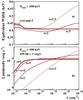 |
Fig. 1 Calculated a) EW and b) luminosity of the 6.4 keV Fe Kα line produced by LECR electrons as a function of the path length of the primary electrons injected in the X-ray production region, for five values of the electron spectral index s (Eq. (A.7)). The ambient medium is assumed to have a solar composition and the electron minimum energy Emin = 100 keV. In panel b), the luminosity calculations are normalized to a total power of 1 erg s-1 injected by the fast primary electrons in the ambient medium. |
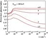 |
Fig. 2 Slope at 6.4 keV of the bremsstrahlung continuum emission produced by LECR electrons, as a function of the path length of the primary electrons injected in the X-ray production region, for five values of the spectral index s. The electron minimum energy is taken to be Emin = 100 keV. |
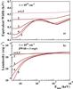 |
Fig. 3 Same as Fig. 1 but as a function of the electron minimum energy, for Λ = 1025 cm-2. |
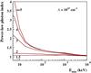 |
Fig. 4 Same as Fig. 2 but as a function of the electron minimum energy, for Λ = 1025 cm-2. |
We present in Figs. 1–4 characteristic properties of the X-ray spectrum resulting from LECR electron interactions around the neutral Fe Kα line. All the calculations were performed for an ambient medium of solar composition (i.e. Z = Z⊙ where Z⊙ is the solar metallicity). Figures 1 and 3 show the equivalent width (EW) and luminosity of the 6.4 keV line, whereas Figs. 2 and 4 show the slope of the underlying continuum emission at the same energy. The former two quantities depend linearly on the metallicity, whereas the continuum emission, which is produced by electron bremsstrahlung in ambient H and He, is independent of Z.
We see in Figs. 1a and 3a that the EW of the Fe Kα line is generally lower than ~0.45 × (Z / Z⊙) keV. The only exception is for s = 1.5 and Λ > 1024 cm-2. But in all cases, we expect the EW to be lower than 0.6 × (Z / Z⊙) keV. This result constitutes a strong constraint for a possible contribution of LECR electrons to the 6.4 keV line emission from the GC region, because the observed EW is >1 keV in some places (see Sect. 5) and sometimes equal to ~2 keV (see, e.g., Revnivtsev et al. 2004).
The results shown in Figs. 1a and 3a were obtained without considering the additional fluorescent line emission that can result from photoionization of ambient Fe atoms by bremsstrahlung X-rays > 7.1 keV emitted in the cloud. This contribution can be estimated from the Monte-Carlo simulations of Leahy & Creighton (1993), who studied the X-ray spectra produced by reprocessing of a power-law photon source surrounded by cold matter in spherical geometry. For the power-law photon index α = 1, the simulated EW of the neutral Fe Kα line can be satisfactorily approximated by 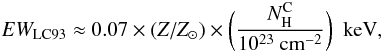 (1)as long as the radial column density of the absorbing cloud,
  , is lower than 1024 cm-2. For α = 2, we have
  keV. Thus, we see by comparing these results with those shown in Figs. 1a and 3a that the additional contribution from internal fluorescence is not strong for
  cm-2.
cm-2.
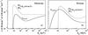 |
Fig. 5 Cross sections involved in the calculation of the Fe Kα line EW. Solid lines: cross sections (in units of barn per ambient H-atom) for producing the 6.4 keV line by the impact of fast electrons (left panel) and protons (right panel), assuming solar metallicity. Dashed lines: differential cross section (in barn per H-atom per keV) for producing 6.4 keV X-rays by bremsstrahlung of fast electrons (left panel) and inverse bremsstrahlung from fast protons (right panel), in a medium composed of H and He with H/He = 0.1. The ratio of these two cross sections gives the EW of the 6.4 keV line (in keV) for a mono-energetic beam of accelerated particles. |
As shown in Figs. 1b and 3b, the production of 6.4 keV line photons by LECR electron interactions is relatively inefficient: the radiation yield R6.4 keV = LX(6.4 keV) / (dWe / dt) is always lower than 3 × 10⁻⁶ (Z / Z⊙), which implies that a high kinetic power in CR electrons should generally be needed to produce an observable Kα line from neutral or low-ionized Fe atoms. For example, the total luminosity of the 6.4 keV line emission from the inner couple of hundred parsecs of our Galaxy is >6 × 1034 erg s-1 (Yusez-Zadeh et al. 2007), such that dWe / dt > 2 × 1040 erg s-1 would be needed if this emission was entirely due to LECR electrons (assuming the ambient medium to be of solar metallicity). Such power would be comparable to that contained in CR protons in the entire Galaxy.
On the other hand, Fig. 1b shows that LECR electrons can produce a significant Fe Kα line (i.e. R6.4 keV ~ 10-6) in diffuse molecular clouds with  cm-2, especially in the case of strong particle diffusion for which Λ can be much larger than (see Appendix A). An observation of a 6.4 keV line emission from a cloud with
  cm-2 would potentially be a promising signature of LECR electrons, since the efficiency of production of this line by hard X-ray irradiation of the cloud would be low: the ratio of the 6.4 keV line flux to the integrated flux in the incident X-ray continuum above 7.1 keV (the K-edge of neutral Fe) is only ~ 10-4 for
  cm-2 (Yaqoob et al. 2010).
Figures 2 and 4 show the slope Γ of the bremsstrahlung continuum emission, as obtained from the derivative of the differential X-ray production rate ∂(dQX / dt) / ∂EX taken at 6.4 keV. We see that, for Emin > 100 keV, Γ is lower than 1.4 regardless of s and Λ. This is because bremsstrahlung X-rays <10 keV are mainly produced by LECR electrons <100 keV, and the equilibrium spectrum of these electrons is hard (see Fig. B.1) and depends only weakly on the distribution of electrons injected in the ambient medium at higher energies.
Thus, after having studied the influence of the free parameters over broad ranges, we can summarize the main characteristics of the X-ray emission produced by LECR electrons as follows. First, the continuum radiation should generally be hard, Γ < 1.4, provided that nonthermal electrons ≲ 100 keV are not able to escape from their acceleration region and penetrate denser clouds. Secondly, the EW of the 6.4 keV Fe Kα line is predicted to be ~(0.3–0.5) × (Z / Z⊙) keV, whatever the electron acceleration spectrum and transport in the ambient medium.
The reason that the EW of the 6.4 keV line is largely independent of the electron energy distribution is given in Fig. 5a, which shows the relevant cross sections for this issue. The solid line is the cross section for producing 6.4 keV Fe Kα X-rays expressed in barn per ambient H-atom, that is  (see Eq. (B.3)). The dashed line is the differential cross section for producing X-rays of the same energy by electron bremsstrahlung. The Fe line EW produced by a given electron energy distribution is obtained from the ratio of the former cross section to the latter, convolved over that distribution. We see that the two cross sections have similar shapes, in particular similar energy thresholds, which explains why the EW of the 6.4 keV line depends only weakly on the electron energy. However, the cross section for producing the 6.4 keV line increases above 1 MeV as a result of relativistic effects in the K-shell ionization process (Quarles 1976; Kim et al. 2000b), which explains why the EW slightly increases with the hardness of the electron source spectrum (see Fig. 3a).
Figure 5b shows the same cross sections but for proton impact. The calculation of these cross sections are presented in Appendix C. We see that the cross section for the line production has a lower energy threshold than that for the bremsstrahlung continuum. We thus expect that LECR protons with a relatively soft source spectrum can produce a higher EW of the 6.4 keV line than the electrons (see also Dogiel et al. 2011).
2.2. LECR ions
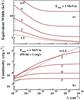 |
Fig. 6 Calculated a) EW and b) luminosity of the 6.4 keV Fe Kα line produced by LECR ions as a function of the path length of the CRs injected in the X-ray production region, for five values of the CR source spectral index s (Eq. (A.7)). The ambient medium is assumed to have a solar composition, and the minimum energy of the CRs that penetrate this medium is Emin = 1 MeV nucleon-1. In panel b) the luminosity calculations are normalized to a total power of 1 erg s-1 injected by the fast primary protons in the ambient medium. |
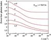 |
Fig. 7 Slope at 6.4 keV of the continuum emission produced by LECR ions as a function of the path length of the fast ions in the X-ray production region, for five values of the spectral index s. The minimum energy of injection is taken to be Emin = 1 MeV nucleon-1. |
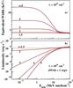 |
Fig. 8 Same as Fig. 6 but as a function of the minimum energy of injection, for Λ = 1025 cm-2. |
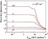 |
Fig. 9 Same as Fig. 7 but as a function of the minimum energy of injection, for Λ = 1025 cm-2. |
Figures 6–9 present characteristic properties of the X-ray spectrum resulting from LECR ion interactions around the neutral Fe Kα line. As before, all the calculations were done for an ambient medium of solar composition. The most remarkable result is that fast ions with a soft source spectrum can produce very high EW of the 6.4 keV line (Figs. 6a and 8a). However, we see in Fig. 8a that the line EW becomes almost independent of s for Emin ≳ 20 MeV nucleon-1. This is because (i) the cross section for producing continuum X-rays at 6.4 keV and the one for the neutral Fe Kα line have similar shapes above 20 MeV nucleon-1 (see Fig. 5b) and (ii) the CR equilibrium spectrum below Emin only weakly depends on s and Λ.
As shown in Fig. 6b, for Emin = 1 MeV nucleon-1, the radiation yield R6.4 keV can reach ~10-6 only for relatively hard source spectra with s ≤ 2 and for Λ ≳ 1025 cm-2, which should generally mean strong particle diffusion in the X-ray production region. For such a high CR path length, the X-rays are mainly produced in thick-target interactions. An efficiency of ~10-6 in the production of the 6.4 keV line can also be achieved with a softer CR source spectrum, if Emin is in the range 10–100 MeV nucleon-1 (Fig. 8b). This is because then most of the CRs are injected into the X-ray production region at energies where the cross section for producing Fe Kα X-rays is highest (see Fig. 5b). But in any case, we find that to get R6.4 keV ~ 10-6 it requires Λ ≳ 1024 cm-2 (for solar metallicity). It is another difference from the production of nonthermal X-rays by LECR electrons, for which R6.4 keV can reach ~10-6 for Λ as low as 1022 cm-2 (Fig. 1b).
Figures 7 and 9 show that the characteristic power-law slope of the continuum emission around 6.4 keV can vary from ~1 to ~6 for s in the range 1.5–5. However, for s ≤ 2, which is expected for strong shock acceleration of nonrelativistic particles, and Λ > 1024 cm-2, which can result from strong particle diffusion in the cloud, we expect Γ between 1.3 and 2. For these conditions, the EW of the neutral Fe Kα line is predicted to be in the narrow range (0.6–0.8) × (Z / Z⊙) keV (Figs. 6a and 8a). This result could account for EW ≳ 1 keV as observed from regions near the GC, provided that the diffuse gas there has a super-solar metallicity (i.e. Z > Z⊙).
3. XMM-Newton observations and data reduction
3.1. Data reduction and particle background substraction
Summary of the XMM-Newton/EPIC observations available for the Arches cluster.
For our analysis, we have considered all public XMM-Newton EPIC observations encompassing the Arches cluster (RA = 17h45m50s, Dec = –28˚49′20′′). The criteria were to have more than 1.5 ks observation time available for each camera, to be in full frame or extended full frame mode, and to use the medium filter. The data was reduced using the SAS software package, version 10.0. Calibrated-event files were produced using the tasks EMCHAIN for the MOS cameras and EPPROC for the pn camera. We excluded from the analysis the period contaminated by soft proton flares, by using an automatic 3σ-clipping method (Pratt & Arnaud 2003). Table 1 provides the list of the 22 selected observations and their respective observing time per instrument after flare rejection.
We searched for any anomalous state of MOS CCD chips (Kuntz & Snowden 2008) by performing a systematic inspection of the images and spectra of each chip in the 0.3–1 keV energy band. We identified 14 occurrences of a noisy chip in the list of observations (see Table 1). The chips affected in our observations by a high-level, low-energy background state are CCD 4 of MOS 1 and CCD 5 of MOS 2. We excluded data of those chips from our analysis when they were noisy.
For MOS cameras, we selected events with PATTERN ≤ 12. Only events with PATTERN ≤ 4 were kept for the pn instrument. Depending on the nature of the analysis, we defined two kinds of quality-flag selection:
-
for imaging, to select events with good angular reconstruction,we used the flags XMMEA_EM and XMMEA_EP for the MOS andpn cameras, respectively;
-
for the spectrum analysis, we chose events with FLAG = XMMEA_SM for MOS cameras (good energy reconstruction) and with FLAG = 0 for the pn camera.
The particle background was derived from filter-wheel closed (FWC) observations that were compiled until revolution about 1600. To be consistent, we applied exactly the same event selection criteria to both data and FWC files. We checked that even if the particle flux has increased significantly between 2000 and 2009, its spectrum and spatial repartition have not significantly changed during that period. We used the count rates between 10 and 12 keV for MOS and between 12 and 14 keV for pn to normalize the FWC background level to that of our observations. Regions with bright sources in the observations have been excluded to calculate the normalization factor. Finally, the EVIGWEIGHT task was used to correct vignetting effects (Pratt et al. 2007).
3.2. Maps generation
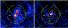 |
Fig. 10 XMM-Newton/EPIC continuum-subtracted Fe Kα emission line maps of the Arches cluster region at 6.4 keV (left panel) and 6.7 keV (right panel). The images have been adaptively smoothed at a signal-to-noise of 20. The magenta circle indicates the region (“Cluster”) used to characterize the Arches cluster X-ray emission, which shows strong Fe Kα emission at 6.7 keV. The region inside the white ellipse but outside the magenta circle indicates the region (“Cloud”) used for spectral extraction to characterize the bright 6.4 keV regions surrounding the Arches cluster. The region inside the yellow circle but outside the two dashed ellipses shows the local background used for the spectral analysis. The axes of the maps (in green) indicate Galactic coordinates in degrees. North is up and east to the left. |
For each observation and instrument, we produced count images (EVSELECT task) in two energy bands (6.3–6.48 keV and 6.564–6.753 keV), which are dominated by the Fe Kα lines at 6.4 keV from neutral to low-ionized atoms and at 6.7 keV from a hot thermally-ionized plasma. For each energy band, observation, and instrument, the normalized particle background image derived from FWC observations was subtracted from the count image. The particle background events were rotated beforehand so as to match the orientation of each instrument for each observation. For each energy band, observation, and instrument, an exposure map was generated (EEXMAP task) taking the different efficiencies of each instrument into account.
To produce line images of the Fe Kα emission at 6.4 and 6.7 keV, the continuum under the line needs to be subtracted. For that, we produced a map in the 4.17–5.86 keV energy band, which is dominated by the continuum emission, with the same procedure as before. To determine the spectral shape of the continuum in the 4–7 keV band, the spectrum of the cloud region (representative region defined in Fig. 10 and Table 2) was fitted by a power law and Gaussian functions to account for the main emission lines. The continuum map was then renormalized to the power-law flux in the considered energy band and subtracted from the corresponding energy band image.
The background-subtracted and continuum-subtracted count images and the exposure maps were then merged using the EMOSAIC task to produce images of the entire observation set. The resulting count images were adaptively smoothed using the ASMOOTH task with a signal-to-noise ratio of 20. The count rate images were obtained by dividing the smoothed count images by the smoothed associated exposure map. The template of the smoothing of the count image was applied to the associated merged exposure map.
Figure 10 shows the resulting Fe Kα line maps at 6.4 and 6.7 keV of the Arches cluster region. The star cluster exhibits strong Fe Kα emission at 6.7 keV. Bright Fe Kα 6.4 keV structures are observed around the Arches cluster.
3.3. Spectrum extraction
To characterize the properties of the emission of the Arches cluster and its surroundings, we defined two regions, which are shown in Fig. 10. The region called “Cluster” corresponds to the Arches cluster and exhibits strong Fe Kα emission at 6.7 keV. The region called “Cloud” corresponds to the bright Fe Kα 6.4 keV emission structures surrounding the Arches cluster. Table 2 provides the coordinates of these regions.
In 9 of the 22 relevant observations, the Arches region lies on the out-of-service CCD6 of MOS 1, reducing the available observation time by more than a factor 2 compared to MOS 2 (see Table 1). Regarding the pn camera, the cloud and cluster regions suffer from the presence of dead columns in a number of observations. We thus estimated the spatial coverage of each region for each pn observation (see Table 1). After several tests, we chose for the spectral analysis to keep only observations with a pn spatial coverage greater than 85%. For all these selected observations, the MOS spatial coverage of each region was greater than 85% (see Table 1).
Table 1 summarizes the final total available exposure time by instrument for spectral analysis. With the 22 observations, we obtained 317 ks for MOS 1 and 652 ks for MOS 2. For the pn spectral analysis, we obtained 276 and 315 ks on the cloud and cluster regions, respectively.
Definition of the spectral extraction regions.
For each region, the particle background spectrum was estimated from the FWC observations in the same detector region. The astrophysical background around the Arches cluster shows spatial structures and, notably, an increase towards the Galactic plane. After several tests, we concluded that the most representative local background for the Arches region was that of the region encircling the Arches, but avoiding the zones emitting at 6.4 keV. The background region is defined in Table 2 and shown in Fig. 10 (yellow circle with the exclusion of the two dashed-line ellipses). To subtract the particle and astrophysical background from the spectra, we used the method of double subtraction described in 3. The ancillary and redistribution matrix function response files were generated with the SAS ARFGEN and RMFGEN tasks, respectively.
The spectra from individual observations of the same region were then merged for each instrument and rebinned to achieve a signal-to-noise per bin of 3σ.
4. Variability of the 6.4 keV line
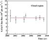 |
Fig. 11 Lightcurve of the 6.4 keV Fe Kα line flux arising from a large region around the Arches cluster (the region labeled “Cloud” in Fig. 10). The red horizontal line shows the best fit with a constant flux. |
The temporal variability of the 6.4 keV line flux is a key diagnostic for deciphering the origin of the line (see, for example, Ponti et al. 2010). To study this aspect, we combined spectra extracted from the cloud region to obtain a sampling of the emission at seven epochs: September 2000 (2 observations), February 2002 (1 observation), March 2004 (2 observations), August/September 2004 (2 observations), March/April 2007 (3 observations), March 2008 (2 observations), and April 2009 (3 observations). This sampling is similar to the one recently used by Capelli et al. (2011b), except that, for an unknown reason, these authors did not included the September 2000 epoch in their analysis.
To measure the intensity of the neutral or low-ionization Fe Kα line at each epoch, we modeled the X-ray emission from the cloud region as the sum of an optically thin, ionization equilibrium plasma (APEC, Smith et al. 2001), a power-law continuum, and a Gaussian line at ~6.4 keV. These three components were subject to a line-of-sight photoelectric absorption so as to account for the high column density of the foreground material. We used the X-ray spectral-fitting program XSPEC1 to fit this model simultaneously to EPIC MOS and pn spectra between 1.5 and 10 keV. More details on the fitting procedure will be given in the next section. All the fits were satisfactory and gave reduced χ2 ~ 1.
The photon fluxes in the 6.4 keV line thus determined are shown in Fig. 11. The best fit of a constant flux to these data is satisfactory, giving a χ2 of 3.3 for six degrees of freedom (d.o.f.). The significance of a variation in the line flux is then only of 0.3σ2. The best-fit mean flux is F6.4 keV = (8.8 ± 0.5) × 10-6 ph cm-2 s-1.
The fact that the intensity of the 6.4 keV line emitted from the vicinity of the Arches cluster is consistent with being constant is in good agreement with the previous work of Capelli et al. (2011b). We note, however, that the line fluxes obtained in the present work are systematically lower by ~20%. This is attributable to a difference in the background modeling: whereas we used a broad region as close as possible to the Arches cluster to subtract the astrophysical background prior to the spectral fitting (Fig. 10), Capelli et al. included the background as a component within the fitting.
5. X-ray spectral analysis of time-averaged spectra
Spectral analysis of the X-ray emission from the Arches star cluster and associated cloud region with standard XSPEC models.
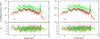 |
Fig. 12 X-ray spectra of the Arches cluster as measured in the MOS1 (black), MOS2 (red), and pn (green) cameras aboard XMM-Newton, compared to a) a model with only one thermal plasma component (model 1 in Table 3) and b) a model with two thermal plasma components (model 3 in Table 3). The lower panels show the associated residuals in terms of standard deviations. The second plasma of temperature kT = 0.9 keV accounts for a significant emission in the He-like Si and S Kα lines at 1.86 and 2.46 keV, respectively. |
We again used XSPEC to fit various models to time-averaged spectra extracted from the two source regions shown in Fig. 10. The fits were performed simultaneously on the stacked MOS1, MOS2, and pn spectra, but we allowed for a variable cross-normalization factor between the MOS and pn data. Independent of the fitting model, we found very good agreement between the MOS and pn cameras, to better than 1% for the data extracted from the cluster region and to 4–5% for the data extracted from the cloud region. These factors are consistent with the residual uncertainty in the flux cross-calibration of the EPIC cameras (Mateos et al. 2009).
5.1. X-ray emission from the star cluster
We first modeled the emission of the cluster region as the sum of an APEC plasma component and a nonthermal component represented by a power-law continuum and a Gaussian line at ~6.4 keV. The centroid energy of the Gaussian line was allowed to vary, but the line width was fixed at 10 eV. All the emission components were subject to a line-of-sight photoelectric absorption (WABS model in XSPEC). The best-fit results obtained with this model (called model 1 in the following) are reported in Table 3 and the corresponding spectra shown in Fig. 12a. In this table and in the following discussion, all the quoted errors are at the 90% confidence level.
This fitting procedure did not allow us to reliably constrain the metallicity of the X-ray emitting plasma. Indeed, the best fit was obtained for a super-solar metallicity Z > 5 Z⊙, which is not supported by other observations. Such an issue has already been faced in previous analyses of the X-ray emission from the Arches cluster region. Thus, Tsujimoto et al. (2007) fixed the plasma metallicity to be solar in their analysis of Suzaku data, whereas Capelli et al. (2011a,b) adopted Z = 2 Z⊙ in their analysis of XMM-Newton data. With the Chandra X-ray Observatory, Wang et al. (2006) were able to resolve three bright point-like X-ray sources in the core of the Arches cluster – most likely colliding stellar wind binaries – and study them individually. These sources were all modeled by an optically thin thermal plasma with a temperature of ~1.8–2.5 keV and a metallicity  . In our analysis, we fixed the metallicity of the thermal plasma in the cluster region to be 1.7 Z⊙, which is the best-fit value that we were able to obtain for the cloud region using the LECR ion model developed in this paper to account for the nonthermal emission (see Sect. 5.2 below). The adopted metallicity is also consistent with the results of Wang et al. (2006).
Model 1 gives a good fit to the data from the cluster region above ~3 keV. In particular, the detection of the neutral or low-ionization Fe Kα line is significant (see Table 3). But the fit is poorer below 3 keV, because the data shows clear excesses of counts above the model at ~1.85 and ~2.45 keV (see Fig. 12a). These features most likely correspond to the Kα lines from He-like Si and S, respectively. We checked that this excess emission is not due to an incomplete background subtraction by producing a Si Kα line image in the energy band 1.76–1.94 keV. To estimate the contribution of the continuum under the Si line, we first produced a count map in the adjacent energy band 2.05–2.15 keV and then normalized it to the expected number of continuum photons in the former energy range. The normalization factor was obtained from a fit to the EPIC spectra of the cluster region by model 1 plus two Gaussian functions to account for the Si and S Kα lines. The resulting map in the Si line shows significant excess emission at the position of the Arches cluster (Fig. 13).
To account for the presence of the He-like Si and S Kα lines in the X-ray spectrum of the cluster, we included in the fitting model a second APEC component subject to the same photoelectric absorption as the other components (model 2). The quality of the fit significantly improves with this additional thermal plasma component (χ2 = 1152 for 976 degrees of freedom), whose best-fit temperature is kT = 0.27 ± 0.04 keV (Table 3). However, the absorption-corrected intrinsic luminosity of this plasma is found to be quite high in the soft X-ray range: Lint(0.4−1 keV) ≈ 2.3 × 1036 erg s-1, assuming the distance to the GC to be D = 8 kpc (Ghez et al. 2008).
In a third model, we let the X-ray emission from the plasma of lower temperature be absorbed by a different column density than the one absorbing the X-rays emitted from the other components. It allows us to further improve the fit to the data (χ2 = 1129 for 975 degrees of freedom, Table 3; see also Fig. 12b for a comparison of this model to the data). We then found  keV and Lint(0.4−1 keV) ≈ 2.0 × 1034 erg s-1 for the lower temperature plasma. The origin of this thermal component, which was not detected in previous X-ray observations of the Arches cluster, is discussed in Sect. 6.1 below.
As can be seen from Table 3, the addition of a second APEC component in the fitting model of the star cluster emission increases the absorbing column density NH(1) significantly. It also has some impact on the temperature of the hotter plasma and on the index of the power-law component, but not on the properties of the 6.4 keV line.
5.2. X-ray emission from the cloud region
We used model 1 to characterize the X-ray emission from the cloud region, except that we also included a Gaussian line at 7.05 keV (fixed centroid energy) to account for the neutral or low-ionization Fe Kβ line. The Fe Kβ/Kα flux ratio was imposed to be equal to 0.13 (Kaastra & Mewe 1993). We checked that including a second thermal plasma component (model 2 or 3) is not required for this region, as it does not improve the quality of the fit. As before, we fixed the metallicity of the emitting plasma to be 1.7 Z⊙. The best-fit temperature,  keV, is marginally higher than the one of the high-temperature plasma emanating from the cluster region.
Spectral analysis of the X-ray emission from the cloud region with LECR electron and ion models.
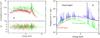 |
Fig. 14 a) X-ray spectra of the cloud region as measured in the XMM-Newton cameras and the best-fit spectral model assuming that the emission comes from a combination of a collisionally ionization equilibrium plasma (APEC model) and a nonthermal component produced by interactions of LECR ions with the cloud constituents (see Table 4); b) model components. |
We now compare the characteristics of the prominent nonthermal emission of the cloud region with the model predictions discussed in Sect. 2. In the LECR electron model, the measured value  would only be expected for low values of the CR minimum energy Emin ≲ 100 keV and for relatively soft source spectra with s ≳ 2.5 (see Fig. 4). But for these CR spectrum parameters the neutral Fe Kα line is predicted to be relatively weak, EW6.4 keV < 0.4 × (Z / Z⊙) keV (see Fig. 3). Thus, it would require an ambient Fe abundance ≳ 3 times the solar value to account for the measured EW of 1.2 ± 0.2 keV. The measured properties of the nonthermal component emitted from the cloud region thus appear to be hardly compatible with the predictions of the LECR electron model.
On the other hand, the measured values of Γ and EW6.4 keV for the cloud region seem to be compatible with the LECR ion model. The measured power-law slope can be produced in this model with any spectral index s ~ 1.5–2, provided that the CR path length Λ > 1024 cm-2 (Figs. 7 and 9). We then expect EW6.4 keV ~ (0.6−1) × (Z / Z⊙) keV (Figs. 6 and 8), which would be in good agreement with the measured EW for an ambient metallicity Z ≲ 2 Z⊙.
To further study the origin of the prominent nonthermal emission of the cloud region, we created LECR electron and ion models that can be used in the XSPEC software. For this purpose, a total of 70 875 spectra were calculated for each model by varying the four free parameters of the models in reasonable ranges. The calculated spectra were then gathered in two FITS files that can be included as external models in XSPEC3. We then fitted the stacked spectra of the cloud region by the XSPEC model WABS × (APEC + LECRp), where p stands for electrons or ions. The best-fit results obtained with both models are given in Table 4.
In this spectral fitting, we allowed for a variable metallicity of the nonthermal X-ray production region (i.e. the parameter Z of the LECRp models), but we imposed this parameter to be equal to the metallicity of the thermal plasma. Since both fits did not usefully constrain the path length of the LECRs in the interaction region, we fixed Λ = 5 × 1024 cm-2 for both models, which, as discussed in Appendix A, is a typical value for nonrelativistic protons propagating in massive molecular clouds of the GC environment (see Eq. (A.6)). As anticipated, the LECR electron model cannot satisfactorily account for the data, because the best fit is obtained for too high a metallicity (Z > 3.1 Z⊙; limit at the 90% confidence level) and a low CR minimum energy (Emin < 41 keV). This conclusion is independent of the adopted value of Λ.
On the other hand, the data can be characterized well by a thin plasma component plus an LECR ion model. In particular, the best-fit metal abundance Z / Z⊙ = 1.7 ± 0.2 is in good agreement with previous works (Wang et al. 2006). The best-fit CR spectral index is  . For such a relatively hard CR source spectrum, one can see from Figs. 8a and 9 that the nonthermal X-ray emission produced by LECR ions only weakly depends on the CR minimum energy Emin. Accordingly, the fit did not constrain this parameter, which was finally fixed at Emin = 10 MeV nucleon-1. As discussed in Appendix A, the process of CR penetration into molecular clouds is not understood well, such that Emin is loosely constrained from theory. This parameter has an effect, however, on the power injected by the primary CRs in the X-ray production region (see Fig. 8b). Thus, for Emin = 1 MeV nucleon-1 (resp. Emin = 100 MeV nucleon-1), the best-fit normalization of the LECR ion model is
 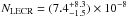 erg cm-2 s-1 (resp.
  erg cm-2 s-1). The corresponding power injected by LECR protons in the cloud region (dW / dt = 4πD2NLECR) lies in the range (0.2–1) × 1039 erg s-1 (with D = 8 kpc).
The best-fit model obtained with the LECR ion component is compared to the data of the cloud region in Fig. 14a, and the corresponding theroretical spectrum is shown in Fig. 14b. The latter figure exhibits numerous lines arising from both neutral and highly-ionized species, which could be revealed by a future instrument having an excellent sensitivity and energy resolution.
6. Origin of the detected radiations
We have identified three distinct components in the X-ray spectra extracted from the cluster region: an optically thin thermal plasma with a temperature kT ~ 1.6–1.8 keV, another plasma of lower temperature (kT ~ 0.3 keV in model 2 or ~0.9 keV in model 3), and a relatively weak nonthermal component characterized by a hard continuum emission and a line at 6.4 keV from neutral to low-ionized Fe atoms (EW6.4 keV = 0.4 ± 0.1 keV). The X-ray radiation arising from the cloud region is also composed of a mix of a thermal and a nonthermal component, but the 6.4 keV Fe Kα line is much more intense from there, with a measured EW of 1.2 ± 0.2 keV.
6.1. Origin of the thermal X-ray emissions
The thermal component of temperature kT ~ 1.6–1.8 keV detected from the star cluster most likely arises from several colliding stellar wind binaries plus the diffuse hot plasma of the so-called cluster wind. Wang et al. (2006) find with the Chandra telescope three point-like sources of thermal emission with kT ~ 1.8–2.5 keV embedded in a spatially extended emission of similar temperature. Capelli et al. (2011a) have recently found with XMM-Newton that the bulk of the X-ray emission from the Arches cluster can be attributed to an optically thin thermal plasma with a temperature kT ~ 1.7 keV. The diffuse thermal emission from the cluster is thought to be produced by the thermalization of massive star winds that merge and expand together. The expected temperature of such a cluster wind is consistent with the temperature of the hot thermal component identified in this and previous works (see Capelli et al. 2011a, and references therein).
The plasma with kT ~ 1.6–1.8 keV is at the origin of the He-like Fe Kα line at 6.7 keV. The corresponding map generated in the present work (Fig. 10, right panel) is in good agreement with the Chandra observations. Wang et al. (2006) suggest that the observed elongation of this emission in the east-west direction reflects an ongoing collision of the Arches cluster with a local molecular cloud traced by the CS emission. As discussed by Wang et al. (2006), this collision may help in explaining the spatial confinement of this hot plasma.
The second thermal component of temperature kT ~ 0.3 keV (model 2) or kT ~ 0.9 keV (model 3) was not detected in previous X-ray observations of the Arches cluster. An optically thin thermal plasma of temperature kT ~ 0.8 keV was reported by Yusef-Zadeh et al. (2002b) from Chandra observations, but not by subsequent X-ray observers (Wang et al. 2006; Tsujimoto et al. 2007; Capelli et al. 2011a). However, the high-quality spectral data obtained in the present work reveal that a single APEC thermal plasma model cannot account simultaneously for the observed lines at ~1.85, ~2.45, and 6.7 keV, which arise from He-like Si, S, and Fe atoms, respectively. The map at ~1.85 keV clearly shows that the star cluster significantly emits at this energy (Fig. 13). The required additional plasma component is subject to a high interstellar absorption: NH ≈ 1.2 × 10²³ in model 2 and 8.3 × 10²² H cm-2 in model 3 (Table 3). It shows that the emitting plasma is located in the Galactic center region and not in the foreground.
The temperature of the second thermal component suggests that this emission could be due to a collection of individual massive stars in the cluster. Single hot stars with spectral types O and early B are known to emit significant amounts of thermal X-rays with a temperature kT in the range 0.1–1 keV and a typical luminosity in soft X-rays LX(0.4−1 keV) ~ 1.5 × 10⁻⁷ Lbol (Antokhin et al. 2008; Güdel & Nazé 2009). Here, Lbol is the bolometric luminosity of the star. The total bolometric luminosity of the Arches cluster is ~107.8 L⊙ and most of it is contributed by early B- and O-type stars, some of which have already evolved to the earliest Wolf-Rayet phases (Figer et al. 2002). Then, a total soft X-ray luminosity LX(0.4−1 keV) ~ 3.6 × 1034 erg s-1 can be expected from the ensemble of hot massive stars of the cluster. This estimate is much lower than the unabsorbed intrinsic luminosity of the ~0.3 keV plasma found in model 2, Lint(0.4−1 keV) ≈ 2.3 × 1036 erg s-1. But it is roughly consistent with the absorption-corrected luminosity of the ~0.9 keV plasma found in model 3: Lint(0.4−1 keV) ≈ 2.0 × 1034 erg s-1. It is not clear, however, why the latter component is less absorbed than the high-temperature plasma emitted from the Arches cluster (Table 3).
6.2. Origin of the 6.4 keV line emission
6.2.1. The cloud region
Several molecular clouds of the GC region emit the 6.4 keV line, most notably Sgr B1, Sgr B2, Sgr C, and clouds located between Sgr A∗ and the Radio Arc (see Yusef-Zadeh et al. 2007). Detections of time variability of the 6.4 keV line from Sgr B2 (Inui et al. 2009), as well as from molecular clouds within 15′ to the east of Sgr A∗ (Muno et al. 2007; Ponti et al. 2010), are best explained by the assumption that the Fe Kα line emission from these regions is a fluorescence radiation produced by the reprocessing of a past X-ray flare from the supermassive black hole Sgr A∗. In this model, the variability of the line flux results from the propagation of an X-ray light front emitted by Sgr A∗ more than ~100 years ago. The discovery of an apparent superluminal motion of the 6.4 keV line emission from the so-called “bridge” region provides strong support for this model (Ponti et al. 2010). The observed line flux variability with a timescale of a few years is hard to explain by a model of CR irradiation.
In contrast to these results, the flux of the neutral or low-ionization Fe Kα line emitted from the Arches cluster vicinity does not show any significant variation over more than eight years of XMM-Newton repeated observations performed between 2000 and 2009 (Sect. 4). Capelli et al. (2011b) divided the zone of 6.4 keV line emission around the cluster into two subregions of about one parsec scale (labeled “N” and “S” by these authors) and found that both subregions emit the line at a constant flux. Other regions in the central molecular zone have been observed to emit a steady 6.4 keV line emission during about the same period, but they generally have larger spatial extents (see, e.g., Ponti et al. 2010). Thus, the spatially averaged Fe Kα emission from Sgr B2 appears to have almost been constant for more than about seven years before fading away (Inui et al. 2009; Terrier et al. 2010), which is compatible with the light crossing time of the molecular cloud complex (see Odaka et al. 2011). But recent observations of Sgr B2 with Chandra suggest that the overall emission of the complex at 6.4 keV is in fact composed of small structures that have constantly changed shape over time (Terrier et al., in prep.).
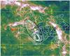 |
Fig. 15 XMM-Newton/EPIC continuum-subtracted 6.4-keV line intensity contours (linearly spaced between 3 × 10⁻⁸ and 1.8 × 10⁻⁷ photons cm-2 s-1 arcmin-2) overlaid with an HST/NICMOS map in the H Paschen-α line (Wang et al. 2010; Dong et al. 2011). The axes of the map indicate Galactic coordinates in degrees. The black ellipse and the magenta circle show the two regions used for spectral extraction (see Fig. 10). The red arrow illustrates the observed proper motion of the Arches cluster, which is almost parallel to the Galactic plane (Stolte et al. 2008; Clarkson et al. 2012). North is up and east to the left. |
Together with the nondetection of time variability, the poor correlation of the spatial distribution of the 6.4 keV line emission with that of the molecular gas also argues against any origin of the Fe line in the Arches cluster region related to Sgr A∗ (Wang et al. 2006). Lang et al. (2001; 2002) studied the position of the molecular clouds in the vicinity of the cluster by combining CS(2–1) observations with H92α recombination line data. The latter were used to trace the Arched filaments H ii regions, which are thought to be located at edges of molecular clouds photoionized by the adjacent star cluster. Lang et al. (2001; 2002) show that the molecular material in this region has a finger-like distribution and that the cluster is located in the midst of the so-called “ − 30 km s-1 cloud” complex, which extends over a region of ~20 pc diameter (see also Serabyn & Güesten 1987).
Figure 15 compares the distribution of the 6.4 keV line emission around the star cluster with a high-resolution image in the hydrogen Paschen-α (Pα) line recently obtained with the Hubble Space Telescope/NICMOS instrument (Wang et al. 2010; Dong et al. 2011). The Pα line emission is a sensitive tracer of massive stars – the Arches cluster is clearly visible in this figure at Galactic coordinates (ℓ,b) ≈ (0.122°,0.018°) – and of warm interstellar gas photoionized by radiation from these stars. The main diffuse Pα-emitting features in Fig. 15 are the three easternmost Arched filaments: E1 (at 0.13° ≲ ℓ ≲ 0.15° and b ~ 0.025°), E2 (at b ≳ 0.04°), and G0.10+0.02 (running from (ℓ,b) ~ (0.09°,0.006°) to (0.1°,0.025°); see also Lang et al. 2002). The 6.4 keV line emission is not well correlated with the Arched filaments. The most prominent structure at 6.4 keV is concentrated in a region of only a few pc2 surrounding the star cluster, much smaller than the spatial extent of the − 30 km s-1 cloud complex. The origin of the faint Fe K emission at (ℓ,b) ~ (0.10°,0.02°) is discusssed in the next section. This strongly suggests that the origin of the bright nonthermal X-ray radiation is related to the cluster itself and not to a distant source such as Sgr A∗.
Assuming that the nonthermal emission from the cloud region is produced by a hard X-ray photoionization source located in the Arches cluster, the 4–12 keV source luminosity required to produce the observed 6.4 keV line flux can be estimated from Sunyaev & Churazov (1998):  (2)where the distance to the GC is again assumed to be 8 kpc. Here, F6.4 keV is the measured 6.4 keV line flux (Table 3), is the column density of the line-emitting cloud, and Ω the fractional solid angle that the cloud subtends at the X-ray source. This quantity is called the covering factor in, e.g., Yaqoob et al. (2010). In comparison, the unabsorbed luminosity of the cluster that we measured from the time-averaged XMM-Newton spectra is LX(4−12 keV) ≈ 5 × 1033 erg s-1. Capelli et al. (2011a) recently detected a 70% increase in the X-ray emission of the Arches cluster in March/April 2007. However, the observed X-ray luminosity of the cluster is about two orders of magnitude short of what is required for the fluorescence interpretation.
An alternative hypothesis is that the 6.4 keV line is produced by a transient photoionization source that was in a long-lasting (>8.5 years) bright state at LX ~ 1036 erg s-1 before a space telescope was able to detect it. No such source was detected with the Einstein observatory in 1979 (Watson et al. 1981) and with subsequent X-ray observatories as well, which imposes a minimum distance of ~4.6 pc between the cloud emitting at 6.4 keV and the putative transient X-ray source. This distance is increased to ~9.2 pc if the cloud and the source are assumed to be at the same line-of-sight distance from the Earth. Furthermore, except for the extraordinarily long outburst of GRS 1915+105, which is predicted to last at least ~20 ± 5 yr (Deegan et al. 2009), the outburst duration of transient X-ray sources is generally much shorter than 8.5 years (see Degenaar et al. 2012). We also note that the Arches cluster is probably too young (t ~ 2.5 yr; Najarro et al. 2004) for an X-ray binary system to have formed within it.
Thus, the 6.4 keV line emission arising from the vicinity of the Arches cluster is unlikely to result from photoionization and is most probably produced by CR impact. We have shown that the measured slope of the nonthermal power-law continuum ( ) and the EW of the 6.4 keV line from this region (EW6.4 keV = 1.2 ± 0.2 keV) are consistent with the predictions of the LECR ion model. On the other hand, LECR electrons cannot satisfactorily account for this emission, because it would require too high metallicity of the ambient gas (Z > 3.1 Z⊙) and too low minimum energy Emin < 41 keV (Table 4). It is indeed unlikely that quasi-thermal electrons of such low energies can escape their acceleration region and penetrate a neutral or weakly ionized medium to produce the 6.4 keV line. We thus conclude that the 6.4 keV line emission from the cloud region is most likely produced by LECR ions.
6.2.2. Are there other processes of production of the 6.4 keV line at work in the Arches cluster region?
A relatively weak line at 6.4 keV is also detected in the spectrum of the X-ray emission from the star cluster. The low EW of this line (EW6.4 keV = 0.4 ± 0.1 keV) may suggest that this radiation is produced by LECR electrons accelerated within the cluster. The existence of a fast electron population there is supported by the detection with the VLA of diffuse nonthermal radio continuum emission (Yusef-Zadeh et al. 2003). The nonthermal electrons are thought to be produced by diffuse shock acceleration in colliding wind shocks of the cluster flow.
It is, however, more likely that the 6.4 keV line detected from this region is produced in molecular gas along the line of sight outside the star cluster. In the Chandra/ACIS 6.4 keV line image of the Arches cluster region, the bow shock-like structure observed in the neutral or low-ionization Fe Kα line covers the position of the star cluster (Wang et al. 2006). The 6.4 keV line emission from the region “Cluster” is not observed in the present map (Figs. 10 and 15), because it has been artificially removed in the process of subtraction of the continuum under the line (see Sect. 5.2). Lang et al. (2002) find evidence of molecular gas lying just in front of the ionized gas associated with the most eastern Arched filament (E1) close to the cluster sight line. According to the geometric arrangement of the −30 km s-1 clouds proposed by these authors, it is likely that the cluster is presently interacting with this foreground molecular gas. From the gradient of visual extinction detected by Stolte et al. (2002) over a field of 40′′ × 40′′ around the star cluster, 9 < ΔAV < 15 mag, the H column density of this cloud along the line of sight can be estimated as  cm-2. The calculations of the present paper show that LECR ions can produce a significant 6.4 keV Fe Kα line emission in such a cloud (Sect. 2), especially in the case of strong particle diffusion for which the CR path length Λ can be much higher than (see Appendix A). It is thus likely that the weak nonthermal X-ray emission detected in the cluster spectrum has the same physical origin as the nonthermal emission from the cloud region.
Relatively faint, diffuse emission in the neutral or low-ionization Fe Kα line is also detected to the west of the Arches cluster, from an extended region centered at (ℓ,b) ~ (0.1°,0.016°) (see Fig. 15). Capelli et al. (2011b) found the light curve of the 6.4 keV line flux from this region (labelled “SN” by these authors) to be constant over the 8-year observation time. With a measured proper motion of ~4.5 mas yr-1 almost parallel to the Galactic plane and towards increasing longitude (Stolte et al. 2008; Clarkson et al. 2012), the Arches cluster was located within this region of the sky ~2 × 10⁴ years ago. It is therefore conceivable that this emission is also due to LECR ions that were accelerated within or close to the cluster at that time. That the nonthermal X-ray emission is still visible today would then indicate that the fast ions have propagated since then in a medium of mean density nH ≲ 103 cm-3. Indeed most of the 6.4 keV line emission from LECR ions is produced by protons of kinetic energies <200 MeV (see Fig. 5b) and the slowing-down time of 200-MeV protons in nH = 103 cm-3 is ~2 × 10⁴ years.
Capelli et al. (2011b) also considered a large region of 6.4 keV line emission located at (ℓ,b) ~ (0.11°,0.075°) (see Fig. 10, left panel). They measured a fast variability of the neutral or low-ionization Fe Kα line from this region and suggest that it could result from the illumination of a molecular cloud by a nearby transient X-ray source. The X-ray emission from this region is not studied in the present paper.
7. Origin of the LECR ion population
Two sites of particle acceleration in the Arches cluster region have been proposed. As already mentioned, Yusef-Zadeh et al. (2003) report evidence of diffuse nonthermal radio synchrotron emission from the cluster and suggest that the emitting relativistic electrons are accelerated by diffuse shock acceleration in the colliding stellar winds of the cluster flow. Another scenario is proposed by Wang et al. (2006), who suggest that the 6.4 keV line emission from this region comes from LECR electrons produced in a bow shock resulting from an ongoing supersonic collision between the star cluster and an adjacent molecular cloud. Both processes could also produce LECR ions.
Since the work of Wang et al. (2006), the apparent proper motion of the Arches cluster in the plane of the sky has been observed with Keck laser-guide star adaptive optics (Stolte et al. 2008; Clarkson et al. 2012). The direction of motion of the cluster stars relative to the field population is represented by the arrow in Fig. 15. The 6.4 keV line emission close to the cluster shows two bright knots connected by a faint bridge to the east of the cluster, i.e. ahead of the moving stars (Fig. 15). The overall structure indeed suggests a bow shock. However, the Fe K line intensity scales as the product of the density of cosmic rays and that of the ambient medium around the cluster, which is probably highly inhomogeneous. A clear bow shock shape is therefore not to be expected. In fact, the 6.4 keV map from this region may also be explained by LECR ions escaping from the cluster and interacting with adjacent molecular gas. Thus, the morphology of the bright structure at 6.4 keV does not allow us to favor one of the two proposed sites for the production of fast ions. But more information can be obtained by studying the CR power required to explain the X-ray emission (Sect. 7.1), as well as the accelerated particle composition (Sect. 7.2).
7.1. CR spectrum and energetics
Whether the main source of LECR ions in the Arches cluster region is the cluster bow shock or colliding stellar winds within the cluster flow, the nonthermal particles are likely to be produced by the diffusive shock acceleration (DSA) process. The nonthermal particle energy distribution resulting from this process can be written for linear acceleration as (e.g. Jones & Ellison 1991)  (3)where p and v are the particle momentum and velocity, respectively, and
  (4)Here, γg is the adiabatic index of the thermal gas upstream the shock front (γg = 5 / 3 for an ideal nonrelativistic gas) and MS = Vs / cS is the upstream sonic Mach number of the shock, whose velocity is Vs. The sound velocity in the upstream gas is
  (5)where k is the Boltzmann constant, T the gas temperature and μmH the mean particle mass. In an interstellar molecular gas of temperature T = 100 K, cS ≈ 0.8 km s-1. For a strong shock verifying Vs ≫ cS, we find from Eq. (4) sDSA ≅ 2, such that the particle spectrum in the nonrelativistic domain is a power law in kinetic energy of index s ≅ 1.5 (see Eq. (3)). Nonlinear effects due to the modification of the shock structure induced by the back-reaction of accelerated ions can slightly steepen the LECR spectrum, such that typically 1.5 < s < 2 (Berezhko & Ellison 1999). The slope of the CR source spectrum that we derived from the X-ray spectral analysis,
  (see Table 4), is consistent with this theory.
The total power acquired by LECR ions in the cloud region can be estimated from the best-fit normalization of the nonthermal X-ray component (NLECR, see Table 4). We find that the power injected by fast primary protons of energies between Emin = 10 MeV and Emax = 1 GeV in the X-ray emitting region is  erg s-1 (still assuming a distance to the GC of 8 kpc). Taking the uncertainty in Emin into account changes the proton power to (0.2–1) × 1039 erg s-1 (see Sect. 5.5). By integration of the CR source spectrum, we find that about 30–60% more power is contained in suprathermal protons with E < Emin, which, by assumption, do not penetrate dense regions of nonthermal X-ray production. Considering the accelerated α-particles with Cα / Cp ≅ 0.1 adds another factor of 40%. The required total CR power finally amounts to (0.5–1.8) × 1039 erg s-1.
7.1.1. Mechanical power available from massive star winds
The total mechanical power contained in the fast winds from massive stars of the cluster can be estimated from near infrared and radio data. Using such observations, Rockefeller et al. (2005) modeled the diffuse thermal X-ray emission from the cluster with 42 stellar wind sources with mass-loss rates in the range (0.3–17) × 10-5 M⊙ yr-1 and a terminal wind velocity of 1000 km s-1. The total mechanical power contained in these 42 sources is 4 × 1038 erg s-1. Of course, only a fraction of this energy reservoir can be converted to CR kinetic energy. We also note that LECR ions produced in the cluster are likely to diffuse away isotropically, such that those interacting with an adjacent molecular cloud emitting at 6.4 keV would probably represent a minority. Thus, the cluster wind is likely not powerful enough to explain the intensity of the nonthermal X-ray emission.
7.1.2. Mechanical power available from the Arches cluster proper motion
The proper motion of the Arches cluster relative to the field star population has recently been measured to be 172 ± 15 km s-1 (Stolte et al. 2008; Clarkson et al. 2012).The cluster is also moving away from the Sun, with a heliocentric line-of-sight velocity of + 95 ± 8 km s-1 (Figer et al. 2002). The resulting three-dimensional space velocity is V∗ ≈ 196 km s-1. To model the form of the bow shock resulting from this supersonic motion, we approximate the cluster as a point source object that loses mass at a rate ṀW = 10-3 M⊙ yr-1 through a wind of terminal velocity VW = 1000 km s-1 (see Rockefeller et al. 2005). The shape of the bow shock is determined by the balance between the ram pressure of the cluster wind and the ram pressure of the ongoing ISM gas. The pressure equilibrium is reached in the cluster direction of motion at the so-called standoff distance from the cluster (see, e.g., Wilkin 1996)  (6)where ρIC ≅ 1.4mpnIC is the mass density of the local ISM. Here, we assume that since the birth of the cluster ~2.5 Myr ago (Figer et al. 2002; Najarro et al. 2004), the bow shock has propagated most of the time in an intercloud medium of mean H density nIC ~ 10 cm-3 (see Launhardt et al. 2002, for a description of the large-scale ISM in the GC region).
The circular area of a bow shock projected on a plane perpendicular to the direction of motion is  (see Wilkin 1996). Thus, the mechanical power processed by the cluster bow shock while propagating in the intercloud medium is
  erg s-1. In comparison, the steady state, mechanical power supplied by supernovae in the inner ~200 pc of the Galaxy is ~1.3 × 1040 erg s-1 (Crocker et al. 2011). LECRs continuously accelerated out of the intercloud medium at the Arches cluster bow shock possibly contribute ~1% of the steady-state CR power in the GC region (assuming the same acceleration efficiency as in supernova remnants).
The initial total kinetic energy of the cluster motion is  erg, where M∗ ~ 5 × 10⁴ M⊙ is the cluster initial total mass (Harfst et al. 2010). This energy would be dissipated in ~4 Myr according to our estimate of PIC.
Most of the interstellar gas mass in the Galactic nuclear bulge is contained in dense molecular clouds with average H densities of nMC ~ 104 cm-3 and a volume filling factor of a few percent (Launhardt et al. 2002). In the region where the Arches cluster is presently located, the volume filling factor of dense molecular gas is even ≳ 0.3 (Serabyn & Güesten 1987). Thus, the probability of a collision between the cluster bow shock and a molecular cloud is strong. The evidence that the cluster is presently interacting with a molecular cloud has already been discussed by Figer et al. (2002) and Wang et al. (2006). This molecular cloud was identified as “Peak 2” in the CS map of Serabyn & Güesten (1987), who estimated its mass to be MMC = (6 ± 3) × 104 M⊙ and mean H density as nMC = (2 ± 1) × 104 cm-3. The corresponding diameter for a spherical cloud is dMC ~ 5.5 pc or 2.4′ at a distance of 8 kpc, which is consistent with the apparent size of the cloud (Serabyn & Güesten 1987).
The total kinetic power processed in this collision is given by  (7)where ρMC ≅ 1.4mpnMC, VMC is the velocity of the molecular cloud projected onto the direction of motion of the Arches cluster, and AC the area of the contact surface between the “Peak 2” cloud and the bow shock. The latter quantity is not well known. We assume that it is equal to the area of the large region around the cluster emitting in the 6.4 keV line (i.e., the region labeled “Cloud” in Fig. 10 and Table 2): AC = 7 pc2.
The cloud-projected velocity VMC obviously depends on the orbital path of the molecular cloud about the GC. By studying the velocity field of the molecular gas around the Arches cluster, Lang et al. (2001; 2002) obtained constraints on the trajectory of the − 30 km s-1 clouds. They find that the cloud complex likely resides on the far side of the GC, either on a x2 orbit (a noncircular orbit family set up in response to the Galaxy’s stellar bar) or on a trajectory directed towards Sgr A∗ (the cloud complex would then be radially infalling into the supermassive black hole) or perhaps on a trajectory midway between the two situations. If the “Peak 2” cloud resides on an x2 orbit in the back of the Galaxy, the collision of this cloud with the Arches cluster is almost frontal (see Stolte et al. 2008; Clarkson et al. 2012), and VMC is close to the x2 orbital speed vorb ~ 80 km s-1 (see, e.g., Molinari et al. 2011). But if the cloud is radially infalling towards the supermassive black hole, given the radial velocity of the cloud (vrad ≈ − 30 km s-1) and the radial and transverse velocity components of the Arches cluster (vrad ≈ +95 km s-1 and vtrans ≈ + 172 km s-1 directed towards positive longitude; see Clarkson et al. 2012), one finds that VMC ~ 20 km s-1. Thus, depending on the exact cloud trajectory VMC ≈ 50 ± 30 km s-1, which, together with V∗ ≈ 196 km s-1, gives PMC ~ 2.3 × 1040 erg s-1 from Eq. (7).
In comparison, the CR power needed to explain the X-ray observations is dW / dt = (0.5–1.8) × 1039 erg s-1, such that the required particle acceleration efficiency in the bow shock system amounts to a few percent. This is a typical efficiency in the DSA theory and in the phenomenology of the acceleration of the Galactic CRs in supernova remnant shocks, as well (see, e.g., Tatischeff 2008, and references therein). However, a detailed study of the particle acceleration process at work in this peculiar shock system would go beyond the scope of this paper.
The collision kinetic power estimated above is comparable to the steady-state, mechanical power due to supernovae in the inner Galaxy, ~1.3 × 1040 erg s-1 (Crocker et al. 2011). But the typical time duration of a collision between the Arches cluster bow shock and a molecular cloud is expected to be only ~3 × 10⁴ yr, assuming that the size dMC ~ 5.5 pc is typical of the highly-fragmented dense molecular gas of the GC region. The mechanical energy released in such a collision is then ~1052 erg, i.e. comparable to the cluster initial total kinetic energy. Thus, the cluster bow shock very likely has collided no more than once with a molecular cloud since the cluster birth ~2.5 Myr ago. Such a collision can briefly release in the ISM a power in LECRs comparable to the steady-state CR power supplied by supernovae in the GC region (Crocker et al. 2011).
The ISM volume swept up by the Arches cluster bow shock since the cluster birth can be estimated as  (8)where t∗ = 2.5 Myr is the estimated cluster age. This volume represents less than 1% of the total volume of the Galactic nuclear bulge, VNB ~ 1.5 × 10⁷ pc3. In comparison, the volume filling factor of dense molecular cloud in the inner ~230 pc of the Galaxy is a few percent (Launhardt et al. 2002). It is thus likely that the star cluster did not experience any interaction with a molecular cloud before the one with the “Peak 2” cloud that is presently observed.
Simulated orbits of the Arches cluster about the GC suggest that the cluster formed in the front of the Galaxy near an x2 orbit (Stolte et al. 2008). That the Arches cluster presently interacts with a molecular cloud located behind the GC shows that the cluster’s orbit is retrograde to the general motion of stars and gas clouds in the bar potential (see Fig. 8 of Stolte et al. 2008). According to the simulation of possible orbits, the cluster has performed about half a revolution around the GC since its formation, which may have brought it near the far side of the elliptical ring of dense molecular clouds recently studied with the Herschel satellite (Molinari et al. 2011). In this environment, the probability of a collision between the cluster and a molecular cloud has become strong.
7.2. Accelerated ion composition
Fast C and heavier ions can emit very broad X-ray lines resulting from 2p to 1s (Kα) and 3p to 1s (Kβ) in-flight transitions. The 2p and 3p orbital states can be populated either by electron capture from ambient atoms (i.e. charge exchange) or by excitation of 1s electrons for fast ions having one or two electrons. To study the composition of the energetic ions accelerated near the Arches cluster, we developed new LECR ion models that include the line emission of fast C, N, O, Ne, Mg, Si, S, and Fe. We used the tables of K X-ray differential multiplicities,  , given in Tatischeff et al. (1998). This quantity is defined as the number of photons emitted in the Kk line by the projectile i as it slows down over the differential kinetic energy interval dE, owing to interactions with all the constituents of the ambient medium. In the adopted steady-state, slab interaction model, the X-ray line production rate is then simply given by
 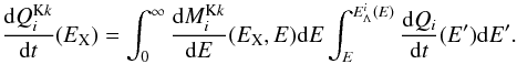 (9)The energy of the emitted X-rays depends on both the velocity and spatial distributions of the fast ions through the usual Doppler formula. We assumed isotropic propagation of the LECRs in the interaction region, which leads to a maximum broadening of the lines.
We note that the calculations of Tatischeff et al. (1998) were done for an ambient medium of solar composition. Nevertheless, their multiplicity results can be used in good approximation for a medium of order twice solar metallicity, since it was found that most of the line emission from the fast ions is produced by interactions with ambient H and He.
We first developed an X-ray production model in which the abundances of the heavy ions are in solar proportions relative to each other, but can vary with respect to H and He, that is (see also Eq. (A.7)) 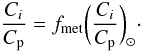 (10)The parameter fmet adds to the spectral index s and the metallicity of the ambient medium Z as a free parameter of the model. But here, we fixed Emin = 10 MeV and Λ = 5 × 1024 cm-2, as in Sect. 5.2. The resulting model was made readable in XSPEC and then used to fit the XMM-Newton spectra extracted from the cloud region. As before, we chose to fit to the data the global XSPEC model WABS × (APEC + LECRi). The best fit was obtained for
  . The corresponding χ2 and best-fit values of the other parameters are nearly the same as in Table 4, in particular with Z / Z⊙ = 1.7 ± 0.2 and
  . The obtained limit at the 90% confidence level fmet < 15.2 shows that the heavy ion abundance is not well constrained by this model.
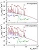 |
Fig. 16 Calculated X-ray emission produced by LECR ions with the spectral parameters s = 1.9, Emin = 10 MeV nucleon-1, and the escape path length Λ = 5 × 1024 cm-2, interacting in a gas cloud of metallicity Z = 1.7 Z⊙ (as obtained in Sect. 5). In panel a) the abundances of the accelerated heavy ions are in solar proportion, but with a metallicity enhancement factor relative to the solar system (SS) composition (see text) fmet = 1 (dashed curve) and fmet = 10 (solid and dotted curves). Panel b) same but for the CRS composition (see text). The dotted curves show the effect of photoelectric absorption on the X-ray spectra for a H column density of 1023 cm-2. |
Figure 16a shows calculated X-ray spectra for the solar system composition with fmet = 1 and 10. We see that intense broad lines can be emitted below 1 keV from X-ray transitions in fast C, N, and O. But this line emission cannot be observed from sources in the GC region, because of the strong interstellar photoelectric absorption along the line of sight. With NH ≈ 1023 H cm-2 (Table 4), the main constraint on the accelerated particle composition is provided by a very broad line feature between ~5.5 and 9 keV owing to de-excitations in fast Fe. This emission is produced by Fe ions of energies between ~5 and 20 MeV nucleon-1 (Tatischeff et al. 1998).
In a second model, we assumed that the fast metals have the composition as the current epoch Galactic CRs at their sources. We obtained the CR source (CRS) composition by taking the heavy ion abundances relative to O given by Engelmann et al. (1990) and using the abundance ratios Cα / CO = 19 and Cp / Cα = 15 recommended by Meyer et al. (1997). The resulting CRS composition is consistent with the recent theoretical works of Putze et al. (2011). The Fe abundance in the CRS composition is CFe / Cp = 6.72 × 10⁻⁴, which is 19 times higher than the one in the solar system composition, (CFe / Cp)⊙ = 3.45 × 10⁻⁵ (Lodders et al. 2003). The best fit of this model to the X-ray spectra of the cloud region was obtained for  (i.e. fmet < 0.71 at the 90% confidence level), consistent with the higher abundance of Fe in the CRS composition. X-ray spectra calculated for this composition are shown in Fig. 16b.
The main outputs of this analysis are the nondetection in the X-ray spectra of the cloud region of a significant excess emission from fast Fe and the implication that CFe / Cp ≲ 5 × 10⁻⁴. This result by itself does not provide strong support for one or the other possible site of acceleration of the LECR ions in the Arches cluster region. Indeed, with the best-fit metallicity Z / Z⊙ = 1.7 ± 0.2, the Fe abundance in the local molecular cloud is aFe = Z / Z⊙ (aFe)⊙ ≈ 5.9 × 10⁻⁵, which is well below the upper limit obtained above. The Fe abundance can be slightly higher in the wind material expelled by the massive stars of the Arches cluster. According to Parizot et al. (1997), one expects in the average composition of the winds from OB associations in the inner Galaxy aFe = 1.4 × 10⁻⁴, which is still below the derived upper limit.
However, the Galactic CRS composition is best described in terms of a general enhancement of the refractory elements such as Fe relative to the volatile ones (Meyer et al. 1997). This selection effect is most likely related to the acceleration process at work in supernova remnant shock waves. Given the limit fmet < 0.71 that we obtained for the CRS composition, we conclude that this effect is weaker in the shock system associated with the Arches cluster proper motion, which according to the energetics arguments discussed in Sect. 6.2.2, is the most likely site of acceleration of the X-ray emitting LECR ions.
8. Cosmic-ray ionization rate
We estimated in Sect. 7.1 that a kinetic power of (0.5–1.8) × 1039 erg s-1 is currently delivered by the Arches cluster bow shock system to LECR ions of energies <1 GeV nucleon-1. The power continuously deposited into the adjacent molecular cloud is lower than that, because of (i) the nonpenetration of CRs with E < Emin into the interaction region and (ii) the escape from the cloud of the highest energy CRs. For Λ = 5 × 1024 cm-2, protons of energies up to 180 MeV are stopped in the cloud, whereas those injected at higher energies do not virtually lose energy in this medium. Taking these effects into account, we find that the power deposited by LECRs into the cloud amounts to Ẇd ~ 4 × 1038 erg s-1. The initial kinetic energy of the fast ions is essentially lost through ionization of the ambient gas and the corresponding ionization rate can be estimated to be 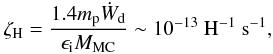 (11)where ϵi ≈ 40 eV is the mean energy required for a fast ion to produce a free electron in a neutral gas mixture of H2 and He in cosmic proportion (Dalgarno et al. 1999) and MMC = (6 ± 3) × 104 M⊙ is the cloud mass (Serabyn & Güesten 1987). The mean ionization rate induced by LECRs in this molecular cloud is significantly higher than the mean ionization rate in the GC region, ζH ≳ 10-15 H-1 s-1 (see Crocker et al. 2011, and references therein).
By integrating the differential equilibrium number of LECRs in the X-ray production region (see Eq. (A.1)), we find that the total kinetic energy contained in fast ions diffusing in the cloud is Etot ~ 4 × 1048 erg. The corresponding mean energy density is Etot / VMC ~ 1000 eV cm-3 (here VMC = MMC / (1.4nMCmp)), which is about one thousand times higher than the Galactic CR energy density in the solar neighborhood. Thus, the molecular cloud irradiated by fast particles accelerated near the Arches cluster bow shock shows some similarities with the “extreme CR dominated regions” recently studied by Papadopoulos et al. (2011) in the context of starbursts. Following the works of these authors, LECRs could explain the high temperature of the “Peak 2” cloud measured by Serabyn & Güesten (1987): T ≳ 100 K.
9. Gamma-ray counterparts
Collisions of LECR ions with molecular cloud matter can lead to nuclear excitations of both ambient and accelerated heavy ions followed by emission of de-excitation γ-ray lines (Ramaty et al. 1979; Benhabiles-Mezhoud et al. 2011). We calculated the γ-ray line flux expected from the Arches cluster region using the same CR interaction model as before (see Appendix A), with s = 1.9, Emin = 10 MeV, NLECR = 5.6 × 10⁻⁸ erg cm-2 s-1, Λ = 5 × 1024 cm-2, and Z / Z⊙ = 1.7 (Table 4). The predicted flux is well below the sensitivity limit of the INTEGRAL observatory. For example, we obtain a flux of 2.3 × 10⁻⁸ ph cm-2 s-1 in the 4.44 MeV line from de-excitations of ambient 12C, whereas the sensitivity of the INTEGRAL spectrometer SPI for detection of a narrow line at this energy is >10-5 ph cm-2 s-1.
Nuclear interactions of CR ions with ambient matter can also lead to high-energy γ-ray emission via the production and subsequent decay of π0 mesons. We used the model of Dermer (1986) for this calculation, but multiplied the π0 emissivity given by this author by a factor of 1.27 to be consistent with the local emissivity measured with the Fermi Gamma-ray Space Telescope (Abdo et al. 2009). The high-energy γ-ray flux strongly depends on the shape of the CR energy distribution, because the neutral pions are produced at significantly higher energies than the nonthermal X-rays. We first assumed a CR source spectrum of the form given by Eq. (3) for this calculation (i.e. resulting from the DSA process) with sDSA = 2s − 1 = 2.8 and no high-energy cutoff. We then found that the Arches cluster region would emit a flux of 5.7 × 10⁻⁷ ph cm-2 s-1 in γ-rays of energies >300 MeV. Such high-energy emission would have probably been already detected by Fermi, since the predicted flux is ~1.75 times higher than the flux of the Galactic central source 1FGL J1745.6–2900 (Chernyakova et al. 2011). But an exponential cutoff in the CR distribution can be expected either because of the finite size of the particle acceleration region near the cluster bow shock or the finite time available for particle acceleration. For example, with an exponential cutoff at 0.5 GeV nucleon-1 (resp. 1 GeV nucleon-1), the flux of γ-rays > 300 MeV would be reduced to 1.4 × 10⁻⁸ ph cm-2 s-1 (resp. 5.1 × 10⁻⁸ ph cm-2 s-1) without significantly changing the nonthermal X-ray production. The high-energy γ-ray emission from the Arches cluster region would then be undetectable with Fermi.
10. Summary
We have studied the production of nonthermal line and continuum X-rays by interaction of LECR electrons and ions with a neutral ambient medium in detail. We developed a steady-state, slab model in which accelerated particles penetrate at a constant rate a cloud of neutral gas, where they produce nonthermal X-rays by atomic collisions until they either stop or escape from the cloud. We examined the properties of the neutral Fe Kα line excited by impacts of LECR electrons and ions. The predicted line EW and luminosity, as well as the slope of the underlying bremsstrahlung continuum, were presented as functions of the free parameters of the model. These results are intended to help observers study the potential role of LECRs for any 6.4 keV line emission and possibly decipher the nature of the nonthermal particles responsible for the line emission. In addition, we generated LECR electron and ion models that can be used in the XSPEC software for more quantitative comparison with data.
We showed, in particular, that the EW of the neutral Fe Kα line excited by LECR electrons is generally expected to be lower than 1 keV, except if the metallicity of the ambient medium exceeds ≈ 2 Z⊙. But LECR ions with a relatively soft source spectrum can lead to a much larger EW. However, the production of 6.4 keV line photons by both LECR electrons and ions is relatively inefficient: the radiation yield R6.4 keV = LX(6.4 keV) / (dW / dt) is typically on the order of 10-6, meaning that a high power in LECRs should generally be needed to produce an observable neutral Fe Kα line.
We then employed the newly developed models to study the X-ray emission emanating from the Arches cluster region. We used all public XMM-Newton EPIC observations encompassing the studied region for our analysis. The main results of this analysis can be summarized as follows.
-
The X-ray flux detected from the Arches cluster is dominated bythe emission of an optically thin thermal plasma with atemperaturekT ~ 1.7 keV. This component most likely arises from the thermalization of massive star winds that merge and expand together, plus the contribution of several colliding stellar wind binaries within the cluster.
-
A second thermal plasma of lower temperature is required to explain the presence of He-like Si and S Kα emission lines in the X-ray spectrum of the cluster. This component, which was not detected in previous X-ray observations, may be produced by a collection of individual massive stars.
-
Bright 6.4 keV Fe Kα line structures are observed around the Arches cluster. We found that the line flux from this region is consistent with its being constant over more than eight years of XMM-Newton repeated observations, in agreement with the recent works of Capelli et al. (2011b). This radiation is unlikely to result from the photoionization of a molecular cloud by a hard X-ray source. It is also probably not produced by LECR electrons, because it would require a metallicity of the ambient gas (Z > 3.1 Z⊙) that is too high. On the other hand, the X-ray emission observed around the cluster can be well-fitted with a model composed of an optically thin thermal plasma and a nonthermal component produced by LECR ions. The best-fit metallicity of the ambient medium found with this model is Z / Z⊙ = 1.7 ± 0.2, and the best-fit CR source spectral index is
. -
The required flux of LECR ions is likely to be produced by the diffusive shock acceleration process in the region of interaction of the Arches cluster and the adjacent molecular cloud identified as “Peak 2” in the CS map of Serabyn & Güesten (1987). We estimated that a total kinetic power of ~2.3 × 1040 erg s-1 is currently processed in the ongoing supersonic collision between the star cluster and the molecular cloud emitting the 6.4 keV line. A particle acceleration efficiency of a few percent in the resulting bow shock system would produce enough CR power to explain the luminosity of the nonthermal X-ray emission.
-
We developed LECR ion models that include the production of broad X-ray lines from fast C and heavier ions following electron captures from ambient atoms (i.e. charge exchanges) and atomic excitations. It allowed us to constrain the abundance of fast Fe ions relative to protons in the LECR ion population: CFe / Cp ≲ 5 × 10⁻⁴. This limit is ~15 times higher than the Fe abundance in the solar system composition.
-
The mean ionization rate induced by LECRs in the molecular cloud that is thought to presently interact with the Arches cluster is ζH ~ 10-13 H-1 s-1. The CR energy density in the interaction region is estimated to be ~1000 eV cm-3, which is about one thousand times higher than the Galactic CR energy density in the solar neighborhood.
-
The high-energy γ-ray emission produced by hadronic collisions between CRs accelerated in the Arches cluster bow shock system and ambient material might be detected with the Fermi Gamma-ray Space Telescope. It crucially depends, however, on the unknown shape of the CR energy distribution above ~1 GeV nucleon-1.
The nonthermal X-ray emission emanating from the Arches cluster region probably offers the best available signature currently for a source of low-energy hadronic cosmic rays in the Galaxy. Deeper observations of this region with X-ray telescopes would allow better characterization of the acceleration process and the effects of LECRs on the interstellar medium. The theory presented in this paper could also be useful for identifying new sources of LECRs in the Galaxy.
Online material
Appendix A: Cosmic-ray interaction model
We consider a model in which low-energy cosmic rays (LECRs) are produced in an unspecified acceleration region and penetrate a nearby cloud of neutral gas at a constant rate (see Fig. A.1). The energetic particles can produce nonthermal X-rays by atomic collisions while they slow down by ionization and radiative energy losses in the dense cloud. We further assume that the LECRs that penetrate the cloud can escape from it after an energy-independent path length Λ, which is a free parameter of the model. The differential equilibrium number of primary CRs of type i (electrons, protons, or α particles) in the cloud is then given by ![Mathematical equation: \appendix \setcounter{section}{1} \begin{equation} N_i (E) = {1 \over [{\rm d}E/{\rm d}t(E)]_i} \int_{E}^{E_\Lambda^i(E)} {{\rm d}Q_i \over {\rm d}t} (E') {\rm d}E', \label{eq1} \end{equation}](/articles/aa/full_html/2012/10/aa19016-12/aa19016-12-eq325.png) (A.1)where (dQi / dt) is the differential rate of LECRs injected in the cloud, [dE / dt(E)] i is the CR energy loss rate, and the maximum energy
(A.1)where (dQi / dt) is the differential rate of LECRs injected in the cloud, [dE / dt(E)] i is the CR energy loss rate, and the maximum energy  is related to the escape path length Λ (expressed in units of H atoms cm-2) by
 ![Mathematical equation: \appendix \setcounter{section}{1} \begin{equation} \Lambda = \int_{E}^{E_\Lambda^i(E)} {{\rm d}E' \over [{\rm d}E/{\rm d}N_{\rm H}(E')]_i}, \label{eq2} \end{equation}](/articles/aa/full_html/2012/10/aa19016-12/aa19016-12-eq329.png) (A.2)where
(A.2)where ![Mathematical equation: \appendix \setcounter{section}{1} \begin{equation} \bigg({{\rm d}E \over {\rm d}N_{\rm H}}\bigg)_i = {1 \over v_i n_{\rm H}} \bigg({{\rm d}E \over{\rm d}t}\bigg)_i \simeq m_{\rm p} \bigg[ \bigg({{\rm d}E \over {\rm d}x}\bigg)_{i,{\rm H}} + 4 \, a_{\rm He} \bigg({{\rm d}E \over {\rm d}x}\bigg)_{i,{\rm He}} \bigg]\cdot \label{eq3} \end{equation}](/articles/aa/full_html/2012/10/aa19016-12/aa19016-12-eq330.png) (A.3)Here, vi is the particle velocity, nH the mean number density of H atoms in the cloud, mp the proton mass, aHe = 0.0964 the cosmic abundance of He relative to H (Lodders 2003), and (dE / dx)i,H and (dE / dx)i,He the CR stopping powers (in units of MeV g-1 cm2) in ambient H and He, respectively. We used for electrons the stopping-power tables of Berger & Seltzer (1982) below 1 GeV and the relativistic formulae given by Schlickeiser (2002) above this energy. The stopping powers for protons and α-particles were extracted from the online databases PSTAR and ASTAR, respectively (Berger et al. 2005).
(A.3)Here, vi is the particle velocity, nH the mean number density of H atoms in the cloud, mp the proton mass, aHe = 0.0964 the cosmic abundance of He relative to H (Lodders 2003), and (dE / dx)i,H and (dE / dx)i,He the CR stopping powers (in units of MeV g-1 cm2) in ambient H and He, respectively. We used for electrons the stopping-power tables of Berger & Seltzer (1982) below 1 GeV and the relativistic formulae given by Schlickeiser (2002) above this energy. The stopping powers for protons and α-particles were extracted from the online databases PSTAR and ASTAR, respectively (Berger et al. 2005).
The process of CR transport in the cloud, which does not need to be specified in the above formalism, is nevertheless relevant to estimate the escape path length Λ from the cloud size. It is clear that if the cloud medium is not diffusive, because of, e.g., efficient ion-neutral damping of MHD waves, Λ ~ nHLC, where LC is the characteristic size of the cloud. But otherwise, the escape path length, which can then be estimated as 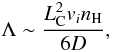 (A.4)can be much greater than the characteristic column density
  , depending on the diffusion coefficient D. For example, with the typical mean diffusion coefficient for the propagation of Galactic CR nuclei in the local interstellar magnetic field B (Berezinsky et al. 1990),
  (A.5)where β = vi / c and Ri is the particle rigidity, one gets from Eq. (A.4) for non-relativistic protons:
  (A.6)where , nH and B are scaled to typical values for massive molecular clouds in the GC region.
For nonrelativistic particles diffusing in the cloud with a diffusion coefficient  typically with 0.3 < sD < 0.5, the escape path length estimated from Eq. (A.4) depends only mildly on energy as Λ ∝ E − sD / 2. However, we have adopted here a simple slab model with an energy-independent escape path length in order to limit the number of free parameters as much as possible.
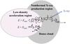 |
Fig. A.1 Schematic illustration of the cosmic-ray interaction model: fast particles produced in a low-density acceleration region can diffusively penetrate a denser cloud (if their kinetic energy is higher than a threshold energy Emin) and then produce nonthermal X-rays by atomic collisions. |
The process of CR penetration into molecular clouds is not well known (see, e.g., Gabici et al. 2007, and references therein). The theoretical predictions range from almost-free penetration (e.g. Cesarsky & Völk 1978) to exclusion of CRs of kinetic energies up to tens of GeV (e.g. Skilling & Strong 1976). Here, for simplicity, we assume that CRs can freely penetrate the clouds if their kinetic energy is higher than a threshold energy Emin, which is another free parameter of the model. We further consider the differential rate of primary CRs that penetrate the nonthermal X-ray production region to be a power law in kinetic energy above Emin:  (A.7)The model finally has four free parameters that can be studied from spectral fitting of X-ray data (see Sect. 5): Λ, Emin, the power-law spectral index s, and the metallicity of the X-ray emitting cloud, Z. The X-ray spectral analysis also provides the CR spectrum normalization Ci, which allows one to estimate the power injected by the primary LECRs into the nonthermal X-ray production region:
  (A.8)In the following, the integration in the above equation is limited to Emax = 1 GeV. Due to CR escape, the power continuously deposited by the fast particles inside the cloud should generally be lower than dWi / dt.
Appendix B: X-rays from accelerated electron interactions
In the framework of the adopted steady-state, slab interaction model, the differential X-ray production rate from collisions of accelerated electrons with the cloud constituents can be written as ![Mathematical equation: \appendix \setcounter{section}{2} \begin{eqnarray} {{\rm d}Q_{\rm X} \over {\rm d}t}(E_{\rm X}) & = & n_{\rm H} \sum_j a_j \int_0^{\infty} {{\rm d}\sigma_{{\rm e}j} \over {\rm d}E_{\rm X}}(E_{\rm X},E) v_{\rm e}(E) \nonumber \\ & & \times~ [ N_{\rm e,p}(E) + N_{\rm e,s}(E) ] {\rm d}E , \label{eq9} \end{eqnarray}](/articles/aa/full_html/2012/10/aa19016-12/aa19016-12-eq353.png) (B.1)where aj is the abundance of element j relative to H in the X-ray emitting cloud, (dσej / dEX) is the differential X-ray production cross section for electron interaction with atoms j, and Ne,p and Ne,s are the differential equilibrium numbers of primary and secondary LECR electrons in the ambient medium, respectively.
(B.1)where aj is the abundance of element j relative to H in the X-ray emitting cloud, (dσej / dEX) is the differential X-ray production cross section for electron interaction with atoms j, and Ne,p and Ne,s are the differential equilibrium numbers of primary and secondary LECR electrons in the ambient medium, respectively.
B.1. Secondary electron production
Primary LECR electrons injected into an interstellar molecular cloud produce secondary electrons mainly from ionization of ambient H2 molecules and He atoms. The corresponding differential production rate of knock-on electrons is given by ![Mathematical equation: \appendix \setcounter{section}{2} \begin{eqnarray} {{\rm d}Q_{\rm e,s} \over {\rm d}t} (E_{\rm s}) & = & n_{\rm H} \int_{2E_{\rm s}}^{\infty} \bigg[ 0.5 {{\rm d}\sigma_{\rm H_2} \over {\rm d}E_{\rm s}}(E_{\rm s},E_{\rm p}) + a_{\rm He} {{\rm d}\sigma_{\rm He} \over {\rm d}E_{\rm s}}(E_{\rm s},E_{\rm p}) \bigg] \nonumber \\ & & \times~ v_{\rm e}(E_{\rm p}) N_{\rm e,p}(E_{\rm p}) {\rm d}E_{\rm p}, \label{eq10} \end{eqnarray}](/articles/aa/full_html/2012/10/aa19016-12/aa19016-12-eq359.png) (B.2)where (dσH2 / dEs) and (dσHe / dEs) are the H2 and He differential ionization cross sections for the production of a secondary electron of energy Es by impact of a primary electron of energy Ep. The lower limit of the integral is 2Es, because the primary electron is by convention the faster of the two electrons emerging from the collision. The maximum possible energy transfer is therefore Es = 0.5(Ep − Bj) ≃ 0.5Ep, where BH2 = 15.43 eV and BHe = 24.59 eV are the electron binding energies of H2 and He, respectively. This convention is consistent with the definition of the stopping powers used throughout this paper (see Eq. (A.3)), which also pertain to the outgoing electron of higher energy.
(B.2)where (dσH2 / dEs) and (dσHe / dEs) are the H2 and He differential ionization cross sections for the production of a secondary electron of energy Es by impact of a primary electron of energy Ep. The lower limit of the integral is 2Es, because the primary electron is by convention the faster of the two electrons emerging from the collision. The maximum possible energy transfer is therefore Es = 0.5(Ep − Bj) ≃ 0.5Ep, where BH2 = 15.43 eV and BHe = 24.59 eV are the electron binding energies of H2 and He, respectively. This convention is consistent with the definition of the stopping powers used throughout this paper (see Eq. (A.3)), which also pertain to the outgoing electron of higher energy.
The differential ionization cross sections are calculated from the relativistic binary encounter dipole (RBED) theory (Kim et al. 1994; 2000b). This successful model combines the binary-encounter theory for hard collisions with the dipole interaction of the Bethe theory for fast incident electrons. For the differential oscillator strengths, we use the analytic fits provided by Kim et al. (1994) for H2 and Kim et al. (2000a) for He. For the average orbital kinetic energy of the target electrons, we take UH2 = 15.98 eV and UHe = 39.51 eV.
By inserting Eq. (A.1) into Eq. (B.2) and using for the electron energy loss rate the expression given in Eq. (A.3), we see that the secondary electron production rate does not depend on the absolute density of H atoms in the ambient medium (nH). This comment also applies to the X-ray production rate, which only depends on the relative abundances aj (see Eq. (B.1)). This important property of the adopted steady-state, slab model will allow us to estimate unambiguously the cosmic-ray power dWi / dt (Eq. (A.8)) from the measured X-ray flux.
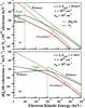 |
Fig. B.1 Calculated differential equilibrium electron numbers (Ne; solid lines) for two differential injection rates of primary electrons (dQe,p / dt; dotted lines): a) s = 3, Emin = 10 keV; b) s = 2, Emin = 1 MeV. Also shown are the differential production rates of secondary, knock-on electrons (dQe,s / dt; dashed lines). The H density in the nonthermal X-ray production region, which intervenes in the calculation of Ne,p and Ne,s, is nH = 104 cm-3 and the path length of the primary electrons in this region is Λ = 1024 cm-2. The calculations are normalized to a total power of 1 erg s-1 injected by the primary LECR electrons in the X-ray production region. |
Calculated differential production rates of primary and knock-on electrons are shown in Fig. B.1. Also shown is the corresponding steady-state differential number of secondary electrons in the ambient medium, Ne,s. We calculated the latter from Eqs. (A.1) and (A.2), assuming the characteristic escape path length of the secondary particles to be Λ/2. Although this assumption is uncertain, it has no significant effect on the total X-ray production.
We see in Fig. B.1 that the effect of H2 and He ionization on the electron energy distribution is to redistribute the total kinetic energy of the injected particles to a larger number of lower-energy electrons. Thus, for hard enough primary electron spectrum (i.e. low s and high Emin, see Fig. B.1b), secondary electrons of energies Es ≳ 10 keV could potentially make a significant contribution to the total nonthermal X-ray emission. On the other hand, one can easily check that the successive production of knock-on electrons by the secondary electrons themselves can be safely neglected for the X-ray emission.
B.2. X-ray continuum emission
The X-ray continuum emission is due to the bremsstrahlung of both primary and secondary electrons. We take electron bremsstrahlung into account only in ambient H and He and calculate the differential cross sections from the work of Strong et al. (2000, Appendix A), which is largely based on Koch & Motz (1959). We use the scattering functions from Blumenthal & Gould (1970) to take into account the arbitrary screening of the H and He nuclei by the bound electrons.
B.3. X-ray line emission
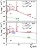 |
Fig. B.2 Calculated X-ray emission produced by LECR electrons with the source spectra shown in Fig. B.1 interacting in a gas cloud of solar metallicity. PEB: primary electron bremsstrahlung; SEB: secondary electron bremsstrahlung. Photoelectric absorption is taken into account with a H column density of 1022 cm-2. |
The X-ray line emission results from the filling of inner-shell vacancies produced by fast electrons in ambient atoms. We consider the Kα and Kβ lines (2p → 1s and 3p → 1s transitions in the Siegbahn notation) from ambient C, N, O, Ne, Mg, Si, S, Ar, Ca, Fe, and Ni. The corresponding cross sections can be written as  (B.3)where EKk is the energy of line Kk (Kα or Kβ), δ(EX − EKk) is Dirac’s delta function,
  the total cross section for the K-shell ionization of atom j by an electron of energy E, and
  the Kk fluorescence yield for atom j (Kaastra & Mewe 1993). Note that
  for element j with atomic number ≤ 12 (i.e. Mg), since these atoms do not have 3p electrons in their ground level.
For the K-shell ionization cross sections, we adopted the semi-empirical formula of Quarles (1976), which agrees well with the RBED cross sections for Ni and lighter elements (see Kim et al. 2000b) and is simpler to use. We checked that the Quarles’s formula correctly reproduces the data compiled in Long et al. (1990), in particular at relativistic energies.
The width of the X-ray lines produced by electron impact can be estimated from the sum of the natural widths of the atomic levels involved in the transition. Indeed, broadening effects caused by multiple simultaneous ionizations can be safely neglected for LECR electrons. Thus, the Kα1 and Kα2 components of the Fe Kα line have experimental full widths at half-maximum (FWHM) of only 2.5 and 3.2 eV, respectively (Salem & Lee 1976). However, the energy separation of the two fine-structure components is 13 eV, which is much less than the energy resolution at 6.4 keV of the X-ray cameras aboard XMM-Newton and Chandra, but larger than the expected resolution of the ASTRO-H X-ray Calorimeter Spectrometer (7 eV FWHM; Takahashi et al. 2010). Here, we neglect the fine-structure splitting of the K lines and for simplicity adopt the same width for all the lines: ΔEX = 10 eV.
Figure B.2 shows calculated nonthermal X-ray spectra (LX = EX × dQX / dt) produced by LECR electrons injected with the differential rates shown in Fig. B.1 into a cloud of solar metallicity. We took the photoelectric absorption of X-rays into account using a H column density NH = 1022 cm-2 and the cross sections of Morrison & McCammon (1983). We see in Fig. B.2 that the most prominent line is that of Fe at 6.40 keV. This is because this element has the highest product of Kα fluorescence yield ( , Kaastra & Mewe 1993) and cosmic abundance. The EW of the Fe Kα line is equal to 293 and 394 eV in the spectra shown in panels a and b, respectively. The second strongest line in these spectra is the Si Kα line at 1.74 keV; its EW is equal to 80 and 90 eV in panels a and b, respectively. We also see in this figure that (i) the shape of the continuum emission reflects the hardness of the primary electron injection spectrum; and (ii) the total X-ray emission is dominated by the contribution of the primary electrons. The emission from the secondary electrons is negligible in panel a and accounts for 10–20% of the total emission below 10 keV in panel b.
Appendix C: X-rays from accelerated ion interactions
The differential X-ray production rate from accelerated ion interactions can be written with a slight modification of Eq. (B.1), as follows: ![Mathematical equation: \appendix \setcounter{section}{3} \begin{eqnarray} {{\rm d}Q_{\rm X} \over {\rm d}t}(E_{\rm X}) & = & n_{\rm H} \sum_j a_j \int_0^{\infty} \bigg[ \sum_i {{\rm d}\sigma_{ij} \over {\rm d}E_{\rm X}} (E_{\rm X},E) v_i(E) N_i(E) \nonumber \\ & & + {{\rm d}\sigma_{{\rm e}j} \over {\rm d}E_{\rm X}}(E_{\rm X},E) v_{\rm e}(E) N_{\rm e,s}(E) \bigg] {\rm d}E , \label{eq13} \end{eqnarray}](/articles/aa/full_html/2012/10/aa19016-12/aa19016-12-eq395.png) (C.1)where the index i runs over the constituents of the nonthermal ion population. The first term in the integral represents the X-ray production by the primary LECR ions and the second term the contribution of the secondary electrons. As a starting point, we assume in the present work that the LECR ion population is mainly composed of protons and α particles and that the contributions of accelerated metals to the total X-ray emission can be neglected. We therefore do not consider the broad X-ray line emission that can arise from atomic transitions in fast C and heavier species following electron captures and excitations (Tatischeff et al. 1998), except in Sect. 7.2. However, for typical compositions of accelerated cosmic particles, the fast metals significantly contribute neither to the production of the X-ray lines from the ambient atoms nor to the bremsstrahlung continuum radiation (see Tatischeff et al. 1998). We further assume that the accelerated protons and α particles are in solar proportion, that is, Cα / Cp = aHe (see Eq. (A.7)).
(C.1)where the index i runs over the constituents of the nonthermal ion population. The first term in the integral represents the X-ray production by the primary LECR ions and the second term the contribution of the secondary electrons. As a starting point, we assume in the present work that the LECR ion population is mainly composed of protons and α particles and that the contributions of accelerated metals to the total X-ray emission can be neglected. We therefore do not consider the broad X-ray line emission that can arise from atomic transitions in fast C and heavier species following electron captures and excitations (Tatischeff et al. 1998), except in Sect. 7.2. However, for typical compositions of accelerated cosmic particles, the fast metals significantly contribute neither to the production of the X-ray lines from the ambient atoms nor to the bremsstrahlung continuum radiation (see Tatischeff et al. 1998). We further assume that the accelerated protons and α particles are in solar proportion, that is, Cα / Cp = aHe (see Eq. (A.7)).
In the calculations of the equilibrium spectra (Np and Nα), we neglect the nuclear destruction and catastrophic energy loss (e.g. interaction involving pion production) of the fast ions in the cloud. Indeed these processes are not important in comparison with the ionization losses below ~300 MeV nucleon-1 kinetic energy (see, e.g., Schlickeiser 2002) and most of the X-ray emission below 10 keV, which is the prime focus of the present work, is produced by ions in this low energy range (see Fig. 5b).
C.1. Secondary electron production
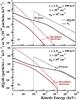 |
Fig. C.1 Calculated differential equilibrium numbers of fast particles (Ni; solid lines) for the differential injection rate of primary protons given by s = 2 and Emin = 100 keV (dQp / dt; dotted lines). Also shown are the differential production rates of secondary knock-on electrons (dQe,s / dt; dashed lines). a) Λ = 1021 cm-2; b) Λ = 1024 cm-2. The H density in the nonthermal X-ray production region is nH = 104 cm-3. The calculations are normalized to a total power of 1 erg s-1 injected by the primary LECR protons in this region. |
We calculate the production of secondary electrons associated to the ionization of ambient H2 molecules and He atoms. The corresponding differential ionization cross sections are obtained as in Tatischeff et al. (1998) from the work of Chu et al. (1981). We neglect the production of secondary electrons and positrons that follows the production of charged pions in hadronic collisions. In fact, the corresponding electron and positron source functions can dominate the one of knock-on electrons only at energies >10 MeV (Schlickeiser 2002), and these high-energy leptons are not important for the production of X-rays <10 keV (see Fig. 5a).
Differential production rates of knock-on electrons are shown in Fig. C.1, together with the corresponding equilibrium spectra of primary protons and secondary electrons. This figure illustrates the effects of changing the CR escape path length from Λ = 1021 cm-2 (panel a) to 1024 cm-2 (panel b). In the first case, protons of energies up to 1.4 MeV are stopped in the cloud, whereas in the second case the transition energy between proton stopping and escape is at 71 MeV. We see that above this transition energy the equilibrium spectrum has a similar slope than the source spectrum, whereas at lower energies the equilibrium proton distribution is harder due to the ionization losses. We can anticipate that the total X-ray production rate will be much higher for the case Λ = 1024 cm-2, as a result of the higher proton number at equilibrium above a few MeV.
C.2. X-ray continuum emission
The X-ray continuum emission is due to inverse bremsstrahlung from the fast ions (the radiation of a single photon in the collision of a high-speed ion with an electron effectively at rest) and classical bremsstrahlung from the secondary knock-on electrons. In the nonrelativistic domain, the bremsstrahlung produced by a proton of kinetic energy E in a collision with a H atom at rest has the same cross section as that of an electron of kinetic energy (me / mp)E in a collision with a stationary proton (me and mp are the electron and proton masses, respectively). We calculate this cross section as in Sect. 3.2, but without taking the screening of the H nucleus by the bound electron into account. The cross section for interaction of a proton with a H atom is then multiplied by (1 + 2aHe) to take the ambient He into account. For α particles, we replace the proton energy E by the energy per nucleon of the projectile and multiply the proton cross section by 4 to account for the nuclear charge dependence of the bremsstrahlung cross section.
In the relativistic case, the cross section for proton inverse bremsstrahlung is different from the one for classical electron bremsstrahlung, owing to the appearance of angular and energy abberations in the transformation between the two rest frames of the interacting particles (Haug 2003). We checked that these effects can be neglected in good approximation in the present work.
In Fig. C.2 we show two X-ray spectra corresponding to the particle equilibrium spectra presented in Fig. C.1. We see that the continuum emission is dominated by inverse bremsstrahlung, which is a general rule independent of the model parameters (see Tatischeff et al. 1998). We also see that, as expected, the X-ray production rate is much higher for Λ = 1024 cm-2 than for Λ = 1021 cm-2, the difference being a factor of 22, 337 and 1054 at 1, 10, and 100 keV, respectively.
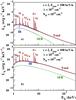 |
Fig. C.2 Calculated X-ray emission produced by LECR protons and α-particles interacting in a gas cloud of solar metallicity, for the differential injection rate of primary protons shown in Fig. 9. The contribution of accelerated α-particles is included as explained in the text, assuming in particular the solar abundance Cα / Cp = 0.0964. a) Λ = 1021 cm-2; b) Λ = 1024 cm-2. IB: inverse bremsstrahlung; SEB: secondary electron bremsstrahlung. Photoelectric absorption is taken into account with a H column density of 1022 cm-2. |
C.3. X-ray line emission
For producing X-ray lines from the ambient atoms, we take both the contribution from secondary electrons (see Eq. (B.3)) and that from primary ions into account. The cross sections for K-shell ionization by proton and α-particle impacts are extracted from the data library implemented by Pia et al. (2009) in the Geant4 toolkit for the simulation of particle induced X-ray emission (PIXE). We use the cross sections calculated in the ECPSSR theory with high-velocity corrections (Lapicki et al. 2008). These cross sections are more accurate for mildly relativistic projectiles than those previously employed by Tatischeff et al (1998).
Proton and α-particle collisions with target atoms do not lead to significant line broadening effects caused by multiple simultaneous ionizations. We thus adopt as before a width of 10 eV for all the lines (see Sect. 3.3). We note, however, that the X-ray lines produced by collisions of ions heavier than 4He can be
shifted by several tens of eV, significantly broadened and split up into several components (Garcia et al. 1973). For example, the Fe Kα line produced by impacts of O ions of 1.9 MeV nucleon-1 is blueshifted by ~50 eV in comparison with the one produced by 5-MeV proton impacts, and has a FWHM of ~100 eV (see Garcia et al. 1973, Fig. 3.55).
The most intense line produced by LECR protons and α-particles is also the neutral Fe Kα line at 6.40 keV (Fig. C.2). This line has an EW of 2.31 and 0.80 keV in the spectra shown in Figs. C.2a and b, respectively. The second strongest line in these spectra is the Si Kα line at 1.74 keV; its EW is equal to 309 eV in panel a and 152 eV in panel b.
Noteworthy is that these results were obtained without taking the systematic error in the effective area of the EPIC camera into account. This error is estimated to be 7% for on-axis sources and to increase with off-axis angle (see the XMM-Newton Calibration Technical Note CAL-TN-0018.pdf at http://xmm.vilspa.esa.es/external/xmm_sw_cal/calib/documentation.shtml).
These models are available upon request to the authors.
Acknowledgments
We would like to thank an anonymous referee for suggestions that helped improve the paper. G.M. acknowledges financial support from the CNES. This work uses observations performed with XMM-Newton, an ESA Science Mission with instruments and contributions directly funded by ESA member states and the USA (NASA).
References
- Abdo, A. A., Ackermann, M., Ajello, M., et al. 2009, ApJ, 703, 1249 [Google Scholar]
- Antokhin, I. I., Rauw, G., Vreux, J.-M., van der Hucht, K. A., & Brown, J. C. 2008, A&A, 477, 593 [NASA ADS] [CrossRef] [EDP Sciences] [Google Scholar]
- Arnaud, M., Majerowicz, S., Lumb, D., et al. 2002, A&A, 390, 27 [NASA ADS] [CrossRef] [EDP Sciences] [Google Scholar]
- Benhabiles-Mezhoud, H., Kiener, J., Thibaud, J.-P., et al. 2011, Phys. Rev. C, 83, 024603 [NASA ADS] [CrossRef] [Google Scholar]
- Berezhko, E. G., & Ellison, D. C. 1999, ApJ, 526, 385 [NASA ADS] [CrossRef] [Google Scholar]
- Berezinskii, V. S., Bulanov, S. V., Dogiel, V. A., & Ptuskin, V. S. 1990, Astrophysical Cosmic Rays, ed. V. L. Ginzburg (North-Holland), Chap. 9 [Google Scholar]
- Berger, M. J., & Seltzer, S. M. 1982, Stopping Powers and Ranges of Electrons and Positrons, National Bureau of Standards report: NBSIR 82-2550, US Dept. of Commerce, Washington, D.C. 20234 [Google Scholar]
- Berger, M. J., Coursey, J. S., Zucker, M. A., & Chang, J. 2005, ESTAR, PSTAR, and ASTAR: Computer Programs for Calculating Stopping-Power and Range Tables for Electrons, Protons, and Helium Ions (version 1.2.3), http://physics.nist.gov/Star, National Institute of Standards and Technology, Gaithersburg, MD [Google Scholar]
- Blumenthal, G. R., & Gould, R. J. 1970, Rev. Mod. Phys., 42, 237 [NASA ADS] [CrossRef] [Google Scholar]
- Capelli, R., Warwick, R. S., Cappelluti, N., et al. 2011a, A&A, 525, L2 [NASA ADS] [CrossRef] [EDP Sciences] [Google Scholar]
- Capelli, R., Warwick, R. S., Porquet, D., Gillessen, S., & Predehl, P. 2011b, A&A, 530, A38 [NASA ADS] [CrossRef] [EDP Sciences] [Google Scholar]
- Cesarsky, C. J., & Volk, H. J. 1978, A&A, 70, 367 [NASA ADS] [Google Scholar]
- Chernyakova, M., Malyshev, D., Aharonian, F. A., Crocker, R. M., & Jones, D. I. 2011, ApJ, 726, 60 [Google Scholar]
- Chu, T. C., Ishii, K., Yamadera, A., Sebata, M., & Morita, S. 1981, Phys. Rev. A, 24, 1720 [NASA ADS] [CrossRef] [Google Scholar]
- Clarkson, W. I., Ghez, A. M., Morris, M. R., et al. 2012, ApJ, 751, 132 [NASA ADS] [CrossRef] [Google Scholar]
- Crocker, R. M., Jones, D. I., Aharonian, F., et al. 2011, MNRAS, 413, 763 [NASA ADS] [CrossRef] [Google Scholar]
- Culhane, J. L., Gabriel, A. H., Acton, L. W., et al. 1981, ApJ, 244, L141 [NASA ADS] [CrossRef] [Google Scholar]
- Dalgarno, A., Yan, M., & Liu, W. 1999, ApJS, 125, 237 [NASA ADS] [CrossRef] [Google Scholar]
- Deegan, P., Combet, C., & Wynn, G. A. 2009, MNRAS, 400, 1337 [NASA ADS] [CrossRef] [Google Scholar]
- Degenaar, N., Wijnands, R., Cackett, E. M., et al. 2012, A&A, 545, A49 [NASA ADS] [CrossRef] [EDP Sciences] [Google Scholar]
- Dermer, C. D. 1986, A&A, 157, 223 [NASA ADS] [Google Scholar]
- Dogiel, V., Cheng, K.-S., Chernyshov, D., et al. 2009, PASJ, 61, 901 [NASA ADS] [CrossRef] [Google Scholar]
- Dogiel, V., Chernyshov, D., Koyama, K., Nobukawa, M., & Cheng, K.-S. 2011, PASJ, 63, 535 [NASA ADS] [Google Scholar]
- Dong, H., Wang, Q. D., Cotera, A., et al. 2011, MNRAS, 417, 114 [NASA ADS] [CrossRef] [Google Scholar]
- Engelmann, J. J., Ferrando, P., Soutoul, A., Goret, P., & Juliusson, E. 1990, A&A, 233, 96 [NASA ADS] [Google Scholar]
- Figer, D. F., Najarro, F., Gilmore, D., et al. 2002, ApJ, 581, 258 [NASA ADS] [CrossRef] [Google Scholar]
- Fukazawa, Y., Hiragi, K., Mizuno, M., et al. 2011, ApJ, 727, 19 [NASA ADS] [CrossRef] [Google Scholar]
- Gabici, S., Aharonian, F. A., & Blasi, P. 2007, Ap&SS, 309, 365 [Google Scholar]
- Garcia, J. D., Fortner, R. J., & Kavanagh, T. M. 1973, Rev. Mod. Phys., 45, 111 [NASA ADS] [CrossRef] [Google Scholar]
- George, I. M., & Fabian, A. C. 1991, MNRAS, 249, 352 [NASA ADS] [CrossRef] [Google Scholar]
- Ghez, A. M., Salim, S., Weinberg, N. N., et al. 2008, ApJ, 689, 1044 [NASA ADS] [CrossRef] [Google Scholar]
- Giardino, G., Favata, F., Pillitteri, I., et al. 2007, A&A, 475, 891 [NASA ADS] [CrossRef] [EDP Sciences] [Google Scholar]
- Güdel, M., & Nazé, Y. 2009, A&ARv, 17, 309 [NASA ADS] [CrossRef] [Google Scholar]
- Hamaguchi, K., Corcoran, M., Gull, T., et al. 2007, ApJ, 663, 522 [NASA ADS] [CrossRef] [Google Scholar]
- Harfst, S., Portegies Zwart, S., & Stolte, A. 2010, MNRAS, 409, 628 [NASA ADS] [CrossRef] [Google Scholar]
- Haug, E. 2003, A&A, 406, 31 [NASA ADS] [CrossRef] [EDP Sciences] [Google Scholar]
- Hellier, C., & Mukai, K. 2004, MNRAS, 352, 1037 [NASA ADS] [CrossRef] [Google Scholar]
- Inui, T., Koyama, K., Matsumoto, H., & Tsuru, T. G. 2009, PASJ, 61, 241 [Google Scholar]
- Jones, F. C., & Ellison, D. C. 1991, Space Sci. Rev., 58, 259 [NASA ADS] [CrossRef] [Google Scholar]
- Kaastra, J. S., & Mewe, R. 1993, A&AS, 97, 443 [NASA ADS] [Google Scholar]
- Kim, Y.-K., & Rudd, M. E. 1994, Phys. Rev. A, 50, 3954, http://physics.nist.gov/PhysRefData/Ionization/index.html [NASA ADS] [CrossRef] [PubMed] [Google Scholar]
- Kim, Y.-K., Johnson, W. R., & Rudd, M. E. 2000a, Phys. Rev. A, 61, 034702 [NASA ADS] [CrossRef] [Google Scholar]
- Kim, Y.-K., Santos, J. P., & Parente, F. 2000b, Phys. Rev. A, 62, 052710 [NASA ADS] [CrossRef] [Google Scholar]
- Koch, H. W., & Motz, J. W. 1959, Rev. Mod. Phys., 31, 920 [NASA ADS] [CrossRef] [Google Scholar]
- Koyama, K., Maeda, Y., Sonobe, T., et al. 1996, PASJ, 48, 249 [NASA ADS] [CrossRef] [Google Scholar]
- Kuntz, K. D., & Snowden, S. L. 2008, A&A, 478, 575 [NASA ADS] [CrossRef] [EDP Sciences] [Google Scholar]
- Lang, C. C., Goss, W. M., & Morris, M. 2001, AJ, 121, 2681 [NASA ADS] [CrossRef] [Google Scholar]
- Lang, C. C., Goss, W. M., & Morris, M. 2002, AJ, 124, 2677 [NASA ADS] [CrossRef] [Google Scholar]
- Lapicki, G. 2008, J. Phys. B At. Mol. Phys., 41, 115201 [NASA ADS] [CrossRef] [Google Scholar]
- Launhardt, R., Zylka, R., & Mezger, P. G. 2002, A&A, 384, 112 [NASA ADS] [CrossRef] [EDP Sciences] [Google Scholar]
- Leahy, D. A., & Creighton, J. 1993, MNRAS, 263, 314 [NASA ADS] [CrossRef] [Google Scholar]
- Lodders, K. 2003, ApJ, 591, 1220 [NASA ADS] [CrossRef] [Google Scholar]
- Long, X., Liu, M., Ho, F., & Peng, X. 1990, At. Data Nucl. Data Tables, 45, 353 [NASA ADS] [CrossRef] [Google Scholar]
- Mateos, S., Saxton, R. D., Read, A. M., & Sembay, S. 2009, A&A, 496, 879 [NASA ADS] [CrossRef] [EDP Sciences] [Google Scholar]
- Meyer, J.-P., Drury, L. O., & Ellison, D. C. 1997, ApJ, 487, 182 [NASA ADS] [CrossRef] [Google Scholar]
- Molinari, S., Bally, J., Noriega-Crespo, A., et al. 2011, ApJ, 735, L33 [NASA ADS] [CrossRef] [Google Scholar]
- Morrison, R., & McCammon, D. 1983, ApJ, 270, 119 [NASA ADS] [CrossRef] [Google Scholar]
- Muno, M. P., Baganoff, F. K., Brandt, W. N., Park, S., & Morris, M. R. 2007, ApJ, 656, L69 [NASA ADS] [CrossRef] [Google Scholar]
- Najarro, F., Figer, D. F., Hillier, D. J., & Kudritzki, R. P. 2004, ApJ, 611, L105 [NASA ADS] [CrossRef] [Google Scholar]
- Odaka, H., Aharonian, F., Watanabe, S., et al. 2011, ApJ, 740, 103 [NASA ADS] [CrossRef] [Google Scholar]
- Osten, R. A., Godet, O., Drake, S., et al. 2010, ApJ, 721, 785 [NASA ADS] [CrossRef] [Google Scholar]
- Papadopoulos, P. P., Thi, W.-F., Miniati, F., & Viti, S. 2011, MNRAS, 414, 1705 [NASA ADS] [CrossRef] [Google Scholar]
- Parizot, E., Cassé, M., & Vangioni-Flam, E. 1997, A&A, 328, 107 [Google Scholar]
- Pia, M. G., Weidenspointner, G., Augelli, M., et al. 2009, IEEE Trans. Nucl. Sci., 56, 3614 [NASA ADS] [CrossRef] [Google Scholar]
- Ponti, G., Terrier, R., Goldwurm, A., Belanger, G., & Trap, G. 2010, ApJ, 714, 732 [NASA ADS] [CrossRef] [Google Scholar]
- Pratt, G., & Arnaud, M. 2003, A&A, 408, 11 [CrossRef] [EDP Sciences] [Google Scholar]
- Pratt, G. W., Böhringer, H., Croston, J. H., et al. 2007, A&A, 461, 71 [NASA ADS] [CrossRef] [EDP Sciences] [Google Scholar]
- Putze, A., Maurin, D., & Donato, F. 2011, A&A, 526, A101 [NASA ADS] [CrossRef] [EDP Sciences] [Google Scholar]
- Quarles, C. A. 1976, Phys. Rev. A, 13, 1278 [NASA ADS] [CrossRef] [Google Scholar]
- Ramaty, R., Kozlovsky, B., & Lingenfelter, R. E. 1979, ApJS, 40, 487 [NASA ADS] [CrossRef] [Google Scholar]
- Revnivtsev, M. G., Churazov, E. M., Sazonov, S. Y., et al. 2004, A&A, 425, L49 [NASA ADS] [CrossRef] [EDP Sciences] [Google Scholar]
- Revnivtsev, M., Sazonov, S., Churazov, E., et al. 2009, Nature, 458, 1142 [NASA ADS] [CrossRef] [PubMed] [Google Scholar]
- Rockefeller, G., Fryer, C. L., Melia, F., & Wang, Q. D. 2005, ApJ, 623, 171 [NASA ADS] [CrossRef] [Google Scholar]
- Salem, S. I., & Lee, P. L. 1976, At. Data Nucl. Data Tables, 45, 353 [Google Scholar]
- Schlickeiser, R. 2002, Cosmic ray astrophysics/Reinhard Schlickeiser, Astronomy and Astrophysics Library, Physics and Astronomy Online Library (Berlin: Springer), ISBN 3-540-66465-3 [Google Scholar]
- Serabyn, E., & Guesten, R. 1987, A&A, 184, 133 [NASA ADS] [Google Scholar]
- Skilling, J., & Strong, A. W. 1976, A&A, 53, 253 [NASA ADS] [Google Scholar]
- Smith, R. K., Brickhouse, N. S., Liedahl, D. A., & Raymond, J. C. 2001, ApJ, 556, L91 [NASA ADS] [CrossRef] [Google Scholar]
- Stolte, A., Grebel, E. K., Brandner, W., & Figer, D. F. 2002, A&A, 394, 459 [NASA ADS] [CrossRef] [EDP Sciences] [Google Scholar]
- Stolte, A., Ghez, A. M., Morris, M., et al. 2008, ApJ, 675, 1278 [NASA ADS] [CrossRef] [Google Scholar]
- Strong, A. W., Moskalenko, I. V., & Reimer, O. 2000, ApJ, 537, 763 [Google Scholar]
- Sunyaev, R., & Churazov, E. 1998, MNRAS, 297, 1279 [NASA ADS] [CrossRef] [Google Scholar]
- Sunyaev, R. A., Markevitch, M., & Pavlinsky, M. 1993, ApJ, 407, 606 [NASA ADS] [CrossRef] [Google Scholar]
- Takahashi, T., Mitsuda, K., Kelley, R., et al. 2010, Proc. SPIE, 7732, 27 [NASA ADS] [Google Scholar]
- Tatischeff, V. 2003, EAS Pub. Ser., 7, 79 [CrossRef] [EDP Sciences] [Google Scholar]
- Tatischeff, V. 2008, in Proc. of Supernovae: lights in the darkness (XXIII Trobades Cientifiques de la Mediterrania), PoS(028) [arXiv:0804.1004] [Google Scholar]
- Tatischeff, V., Ramaty, R., & Kozlovsky, B. 1998, ApJ, 504, 874 [NASA ADS] [CrossRef] [Google Scholar]
- Terrier, R., Ponti, G., Bélanger, G., et al. 2010, ApJ, 719, 143 [NASA ADS] [CrossRef] [Google Scholar]
- Torrejón, J. M., Schulz, N. S., Nowak, M. A., & Kallman, T. R. 2010, ApJ, 715, 947 [NASA ADS] [CrossRef] [Google Scholar]
- Tsujimoto, M., Feigelson, E. D., Grosso, N., et al. 2005, ApJS, 160, 503 [NASA ADS] [CrossRef] [Google Scholar]
- Tsujimoto, M., Hyodo, Y., & Koyama, K. 2007, PASJ, 59, 229 [NASA ADS] [Google Scholar]
- Valinia, A., Tatischeff, V., Arnaud, K., Ebisawa, K., & Ramaty, R. 2000, ApJ, 543, 733 [NASA ADS] [CrossRef] [Google Scholar]
- Vink, J., Kaastra, J. S., & Bleeker, J. A. M. 1997, A&A, 328, 628 [NASA ADS] [Google Scholar]
- Wang, Q. D., Dong, H., & Lang, C. 2006, MNRAS, 371, 38 [NASA ADS] [CrossRef] [Google Scholar]
- Wang, Q. D., Dong, H., Cotera, A., et al. 2010, MNRAS, 402, 895 [NASA ADS] [CrossRef] [Google Scholar]
- Watson, M. G., Willingale, R., Hertz, P., & Grindlay, J. E. 1981, ApJ, 250, 142 [NASA ADS] [CrossRef] [Google Scholar]
- Wilkin, F. P. 1996, ApJ, 459, L31 [NASA ADS] [CrossRef] [Google Scholar]
- Yaqoob, T., Murphy, K. D., Miller, L., & Turner, T. J. 2010, MNRAS, 401, 411 [NASA ADS] [CrossRef] [Google Scholar]
- Yusef-Zadeh, F., Law, C., & Wardle, M. 2002a, ApJ, 568, L121 [NASA ADS] [CrossRef] [Google Scholar]
- Yusef-Zadeh, F., Law, C., Wardle, M., et al. 2002b, ApJ, 570, 665 [NASA ADS] [CrossRef] [Google Scholar]
- Yusef-Zadeh, F., Nord, M., Wardle, M., et al. 2003, ApJ, 590, L103 [NASA ADS] [CrossRef] [Google Scholar]
- Yusef-Zadeh, F., Muno, M., Wardle, M., & Lis, D. C. 2007, ApJ, 656, 847 [NASA ADS] [CrossRef] [Google Scholar]
- Zarro, D. M., Dennis, B. R., & Slater, G. L. 1992, ApJ, 391, 865 [NASA ADS] [CrossRef] [Google Scholar]
All Tables
Spectral analysis of the X-ray emission from the Arches star cluster and associated cloud region with standard XSPEC models.
Spectral analysis of the X-ray emission from the cloud region with LECR electron and ion models.
All Figures
|
Fig. 1 Calculated a) EW and b) luminosity of the 6.4 keV Fe Kα line produced by LECR electrons as a function of the path length of the primary electrons injected in the X-ray production region, for five values of the electron spectral index s (Eq. (A.7)). The ambient medium is assumed to have a solar composition and the electron minimum energy Emin = 100 keV. In panel b), the luminosity calculations are normalized to a total power of 1 erg s-1 injected by the fast primary electrons in the ambient medium. |
| In the text | |
|
Fig. 2 Slope at 6.4 keV of the bremsstrahlung continuum emission produced by LECR electrons, as a function of the path length of the primary electrons injected in the X-ray production region, for five values of the spectral index s. The electron minimum energy is taken to be Emin = 100 keV. |
| In the text | |
|
Fig. 3 Same as Fig. 1 but as a function of the electron minimum energy, for Λ = 1025 cm-2. |
| In the text | |
|
Fig. 4 Same as Fig. 2 but as a function of the electron minimum energy, for Λ = 1025 cm-2. |
| In the text | |
|
Fig. 5 Cross sections involved in the calculation of the Fe Kα line EW. Solid lines: cross sections (in units of barn per ambient H-atom) for producing the 6.4 keV line by the impact of fast electrons (left panel) and protons (right panel), assuming solar metallicity. Dashed lines: differential cross section (in barn per H-atom per keV) for producing 6.4 keV X-rays by bremsstrahlung of fast electrons (left panel) and inverse bremsstrahlung from fast protons (right panel), in a medium composed of H and He with H/He = 0.1. The ratio of these two cross sections gives the EW of the 6.4 keV line (in keV) for a mono-energetic beam of accelerated particles. |
| In the text | |
|
Fig. 6 Calculated a) EW and b) luminosity of the 6.4 keV Fe Kα line produced by LECR ions as a function of the path length of the CRs injected in the X-ray production region, for five values of the CR source spectral index s (Eq. (A.7)). The ambient medium is assumed to have a solar composition, and the minimum energy of the CRs that penetrate this medium is Emin = 1 MeV nucleon-1. In panel b) the luminosity calculations are normalized to a total power of 1 erg s-1 injected by the fast primary protons in the ambient medium. |
| In the text | |
|
Fig. 7 Slope at 6.4 keV of the continuum emission produced by LECR ions as a function of the path length of the fast ions in the X-ray production region, for five values of the spectral index s. The minimum energy of injection is taken to be Emin = 1 MeV nucleon-1. |
| In the text | |
|
Fig. 8 Same as Fig. 6 but as a function of the minimum energy of injection, for Λ = 1025 cm-2. |
| In the text | |
|
Fig. 9 Same as Fig. 7 but as a function of the minimum energy of injection, for Λ = 1025 cm-2. |
| In the text | |
|
Fig. 10 XMM-Newton/EPIC continuum-subtracted Fe Kα emission line maps of the Arches cluster region at 6.4 keV (left panel) and 6.7 keV (right panel). The images have been adaptively smoothed at a signal-to-noise of 20. The magenta circle indicates the region (“Cluster”) used to characterize the Arches cluster X-ray emission, which shows strong Fe Kα emission at 6.7 keV. The region inside the white ellipse but outside the magenta circle indicates the region (“Cloud”) used for spectral extraction to characterize the bright 6.4 keV regions surrounding the Arches cluster. The region inside the yellow circle but outside the two dashed ellipses shows the local background used for the spectral analysis. The axes of the maps (in green) indicate Galactic coordinates in degrees. North is up and east to the left. |
| In the text | |
|
Fig. 11 Lightcurve of the 6.4 keV Fe Kα line flux arising from a large region around the Arches cluster (the region labeled “Cloud” in Fig. 10). The red horizontal line shows the best fit with a constant flux. |
| In the text | |
|
Fig. 12 X-ray spectra of the Arches cluster as measured in the MOS1 (black), MOS2 (red), and pn (green) cameras aboard XMM-Newton, compared to a) a model with only one thermal plasma component (model 1 in Table 3) and b) a model with two thermal plasma components (model 3 in Table 3). The lower panels show the associated residuals in terms of standard deviations. The second plasma of temperature kT = 0.9 keV accounts for a significant emission in the He-like Si and S Kα lines at 1.86 and 2.46 keV, respectively. |
| In the text | |
 |
Fig. 13 Same as Fig. 10 but for the He-like Si Kα line at 1.86 keV. |
| In the text | |
|
Fig. 14 a) X-ray spectra of the cloud region as measured in the XMM-Newton cameras and the best-fit spectral model assuming that the emission comes from a combination of a collisionally ionization equilibrium plasma (APEC model) and a nonthermal component produced by interactions of LECR ions with the cloud constituents (see Table 4); b) model components. |
| In the text | |
|
Fig. 15 XMM-Newton/EPIC continuum-subtracted 6.4-keV line intensity contours (linearly spaced between 3 × 10⁻⁸ and 1.8 × 10⁻⁷ photons cm-2 s-1 arcmin-2) overlaid with an HST/NICMOS map in the H Paschen-α line (Wang et al. 2010; Dong et al. 2011). The axes of the map indicate Galactic coordinates in degrees. The black ellipse and the magenta circle show the two regions used for spectral extraction (see Fig. 10). The red arrow illustrates the observed proper motion of the Arches cluster, which is almost parallel to the Galactic plane (Stolte et al. 2008; Clarkson et al. 2012). North is up and east to the left. |
| In the text | |
|
Fig. 16 Calculated X-ray emission produced by LECR ions with the spectral parameters s = 1.9, Emin = 10 MeV nucleon-1, and the escape path length Λ = 5 × 1024 cm-2, interacting in a gas cloud of metallicity Z = 1.7 Z⊙ (as obtained in Sect. 5). In panel a) the abundances of the accelerated heavy ions are in solar proportion, but with a metallicity enhancement factor relative to the solar system (SS) composition (see text) fmet = 1 (dashed curve) and fmet = 10 (solid and dotted curves). Panel b) same but for the CRS composition (see text). The dotted curves show the effect of photoelectric absorption on the X-ray spectra for a H column density of 1023 cm-2. |
| In the text | |
|
Fig. A.1 Schematic illustration of the cosmic-ray interaction model: fast particles produced in a low-density acceleration region can diffusively penetrate a denser cloud (if their kinetic energy is higher than a threshold energy Emin) and then produce nonthermal X-rays by atomic collisions. |
| In the text | |
|
Fig. B.1 Calculated differential equilibrium electron numbers (Ne; solid lines) for two differential injection rates of primary electrons (dQe,p / dt; dotted lines): a) s = 3, Emin = 10 keV; b) s = 2, Emin = 1 MeV. Also shown are the differential production rates of secondary, knock-on electrons (dQe,s / dt; dashed lines). The H density in the nonthermal X-ray production region, which intervenes in the calculation of Ne,p and Ne,s, is nH = 104 cm-3 and the path length of the primary electrons in this region is Λ = 1024 cm-2. The calculations are normalized to a total power of 1 erg s-1 injected by the primary LECR electrons in the X-ray production region. |
| In the text | |
|
Fig. B.2 Calculated X-ray emission produced by LECR electrons with the source spectra shown in Fig. B.1 interacting in a gas cloud of solar metallicity. PEB: primary electron bremsstrahlung; SEB: secondary electron bremsstrahlung. Photoelectric absorption is taken into account with a H column density of 1022 cm-2. |
| In the text | |
|
Fig. C.1 Calculated differential equilibrium numbers of fast particles (Ni; solid lines) for the differential injection rate of primary protons given by s = 2 and Emin = 100 keV (dQp / dt; dotted lines). Also shown are the differential production rates of secondary knock-on electrons (dQe,s / dt; dashed lines). a) Λ = 1021 cm-2; b) Λ = 1024 cm-2. The H density in the nonthermal X-ray production region is nH = 104 cm-3. The calculations are normalized to a total power of 1 erg s-1 injected by the primary LECR protons in this region. |
| In the text | |
|
Fig. C.2 Calculated X-ray emission produced by LECR protons and α-particles interacting in a gas cloud of solar metallicity, for the differential injection rate of primary protons shown in Fig. 9. The contribution of accelerated α-particles is included as explained in the text, assuming in particular the solar abundance Cα / Cp = 0.0964. a) Λ = 1021 cm-2; b) Λ = 1024 cm-2. IB: inverse bremsstrahlung; SEB: secondary electron bremsstrahlung. Photoelectric absorption is taken into account with a H column density of 1022 cm-2. |
| In the text | |
Current usage metrics show cumulative count of Article Views (full-text article views including HTML views, PDF and ePub downloads, according to the available data) and Abstracts Views on Vision4Press platform.
Data correspond to usage on the plateform after 2015. The current usage metrics is available 48-96 hours after online publication and is updated daily on week days.
Initial download of the metrics may take a while.