© ESO, 2012

1. Introduction

The Tully-Fisher relation (Tully & Fisher 1977, hereafter TFR) is considered one of the most fundamental scaling relations of disc galaxies because it links two important properties: their stellar (sTFR) or baryonic (bTFR) mass content and the depth of their potential well measured by the rotation velocity. Therefore, the study of the TFR at different redshifts (z) could help to trace the dynamics of the gas and the star formation activity within the dark matter haloes, and hence, to provide constraints for galaxy formation models (e.g. Avila-Reese et al. 1998; Mo et al. 1998; Avila-Reese et al. 2008).

The determination of the slope and zero point of the TFR at low (e.g. Bell & de Jong 2001; Pizagno et al. 2007; Meyer et al. 2008; Gurovich et al. 2010) and intermediate and high redshifts (e.g. Conselice et al. 2005; Flores et al. 2006; Atkinson et al. 2007; Kassin et al. 2007; Puech et al. 2008; Cresci et al. 2009; Gnerucci et al. 2011) has been the subject of numerous works. Although many authors suggest the existence of evolution, observational results have not converged yet, and it is also unclear if the evolution is present in the zero point, the slope, or in both (Vogt et al. 1996, 1997; Nakamura et al. 2006). Recent observational results by Miller et al. (2011) show evidence for a modest evolution of the sTFR by 0.04 ± 0.07 from z ~ 1 to z ~ 0.3 in the sense that at a given rotation velocity, galaxies have lower stellar masses in the past. According to the results of Cresci et al. (2009), the sTFR seems to be already in place at z ~ 2 with a slope similar to the local one but displaced towards lower stellar masses by 0.41 ± 0.11 dex. These trends generally agree well with predictions of hydrodynamical simulations (e.g. Portinari & Sommer-Larsen 2007; de Rossi et al. 2010). At higher redshifts, it is not yet clear if the TFR is in place because of the high scatter measured so far (e.g Gnerucci et al. 2011). The origin and evolution of the scatter of the TFR is also considered an open problem. Observational results suggest that it might be driven by systems that exhibit disturbed kinematics as a consequence of galaxy interactions and mergers (Kannappan & Barton 2004; Flores et al. 2006; Puech et al. 2008; Kassin et al. 2007; Covington et al. 2010). Based on previous studies of the TFR (Tully & Fouque 1985), Weiner et al. (2006) proposed a new kinematical estimator generating a combined velocity scale, s_K: ${\mathit{s}}_{\mathrm{K}}^{\mathrm{2}}\mathrm{=}\mathit{K}{\mathit{V}}_{\mathrm{rot}}^{\mathrm{2}}\mathrm{+}{\mathit{\sigma }}^{\mathrm{2}}\mathit{,}$(1)where K is a constant  ≤ 1 and σ is the velocity dispersion. The scale s_K combines rotation (associated to order motion) and pressure support (associated to turbulent and random motion). Kassin et al. (2007) reported that the observed sTFR resulting from the used of s_0.5 is capable of generating a unified relation for galaxies of all morphological types in their sample, including disturbed and merging cases. This TFR based in s_0.5 was also found to be remarkably tight over 0.1 < z < 1.2. By using hydrodynamical pre-prepared merger simulations, Covington et al. (2010) showed that the kinematical indicator s_0.5 correlates with the total potential well of galaxies including baryons and dark matter. A close examination of the kinematical scaling laws of galaxies led these authors to conclude that the appropriate constant K should be  ~ 0.5. Covington et al. (2010) also found that the scatter of the TFR correlates with close encounters and mergers, which suggests that the kinematics could be used to determine the merger stage of the galactic systems (see also Pedrosa et al. 2008). Finally, these authors introduced the kinematical parameter $\mathit{S}\mathrm{=}\sqrt{\mathrm{2}}\mathrm{\times }{\mathit{s}}_{\mathrm{0.5}}$, which seems to be a good tracer of the circular velocity in their simulations. Also, Weiner et al. (2006) proposed a modified version as ${\mathit{s}}_{\mathrm{1.0}}\mathrm{=}\sqrt{{\mathit{V}}_{\mathrm{rot}}^{\mathrm{2}}\mathrm{+}{\mathit{\sigma }}^{\mathrm{2}}}$.

In the current paradigm for galaxy formation, systems assemble hierarchically in a bottom-up fashion so that more massive galaxies are formed by the aggregation of smaller ones. In this scenario, mergers and interactions between galactic systems play a major role in the evolution of baryonic matter within the dark matter potential wells, partially regulating the gas infall and star formation process, which also influence the efficiency of feedback mechanisms. In this context, cosmological N-body/hydrodynamical simulations constitute an ideal tool to follow the evolution of the astrophysical properties of galaxies and may help in understanding the fundamental relations between them. Our simulations were run with a version of GADGET-3, which includes a physically-motivated supernova (SN) feedback (Scannapieco et al. 2006) that is able to trigger mass-loaded gas outflows. This scheme does not require ad hoc mass-dependent parameters but naturally regulates the strength of the SN feedback in haloes of different masses (Scannapieco et al. 2008).

In de Rossi et al. (2010), we studied the sTFR and bTFR in simulated galaxies with very well-defined dominating gaseous discs (disc-to-total gas mass ratios D/T ≥ 0.75) formed in a Λ-CDM universe. We found that both the sTFR and the bTFR are well reproduced by our simulations. Our SN feedback model works in a self-regulated way so that small systems are more strongly affected than large ones. Our simulated sTFR agrees with that recently estimated by Reyes et al. (2011) in the same mass range. While the sTFR is detected to have a bend in the slope for low stellar mass systems as a result of the SN feedback, the bTFR does not show the same feature except at very high redshifts. Accordingly, we found in this previous work that the bTFR does not store information on the impact of SN feedback for reasonable SN energies, except at very early times (z ≈ 3).

In this paper, we extend the work of de Rossi et al. (2010) by studying the gas kinematics of all galaxies with surviving gaseous discs, even those systems dominated by spheroidal components, using the same set of cosmological hydrodynamical simulations. Particular attention is paid to the study of the origin and evolution of the scatter in the TFR, considering the impact of mergers and interactions as well as the importance of gas inflows and outflows. The rotation curves are derived from the analysis of the surviving gaseous discs with the aim at determining the best gas-phase kinematical tracer for the gravitational potential. We assumed that even if the surviving gaseous disc is tenuous, it will trace the potential well that it inhabits.

In Sect. 2, we introduce the numerical simulations studied in this work, the galaxy catalogue, and the methods developed to perform the analysis of gas kinematics. In Sect. 3, we present a discussion of the local TFR and various kinematic gas indicators for galaxies of different morphologies. In Sect. 4, we investigate the fingerprints of the hierarchical aggregation of the structure on the TFR-plane. Our conclusions are summarised in Sect. 5.

2. Numerical experiments

The simulation analysed in this work was performed with the chemical code GADGET-3, an update of GADGET-2 optimised for massive parallel simulations of highly inhomogeneous systems (Springel & Hernquist 2003; Springel 2005). Our version of the code includes treatments for metal-dependent radiative cooling, stochastic star formation, a multiphase model for the interstellar medium (ISM) and an SN feedback scheme (Scannapieco et al. 2005, 2006). The multiphase model allows the coexistence of diffuse and dense gas phases, which improves the description of the ISM (Scannapieco et al. 2006). The SN feedback model is able to trigger mass-loaded galactic outflows without introducing mass-dependent parameters.

The chemical evolution prescription used in this code was developed by Mosconi et al. (2001) and was subsequently adapted by Scannapieco et al. (2005) for GADGET-2. The model describes the enrichment by type II (SNII) and type Ia (SNIa) supernovae according to the chemical yield prescriptions of Woosley & Weaver (1995) and Thielemann et al. (1993), respectively. We adopted a standard Salpeter initial mass function with a lower and upper mass cut-offs of 0.1 M_⊙ and 40 M_⊙, respectively. It was assumed that each SN event generates 0.7 × 10⁵¹ erg. For SNIa, we assumed a time-delay for the ejection of material randomly chosen within  [0.1,1]  Gyr. We assumed that SNII evolved within the same time interval in which they are formed. Metals are distributed within the neighbouring gas particles weighted by the smoothing kernel as proposed by Mosconi et al. (2001).

We used numerical hydrodynamical simulations consistent with a Λ-CDM universe with Ω = 0.3,Λ = 0.7,Ω_b = 0.04, a normalisation of the power spectrum of σ₈ = 0.9 and H₀ = 100   h km s^-1   Mpc^-1 with h = 0.7. Although this set of parameters differs slightly from WMAP-7, the variations have no significant consequences on our results. We simulated a typical field region of the Universe in a comoving cubic volume of 10 Mpc h^-1 side length. Our simulation was run with 2 × 230³ particles, obtaining an initial mass of 9.1 × 10⁵  M_⊙   h^-1 for gas particles, and a mass of 5.9 × 10⁶  M_⊙   h^-1 for the dark matter particles. It is the so-called S230 in de Rossi et al. (2010).

In de Rossi et al. (2010), we showed that the dynamical properties of the galaxies in this sample are robust against numerical resolution and small changes in the parameters of the SN-feedback model. We also found that this simulation predicts correlations between the dynamical properties of galaxies in general good agreement with observations, providing a suitable sample for studying the origin and evolution of the TFR in a cosmological context. In particular, we found that the stellar mass fractions of galaxies residing within dark matter haloes agree well with estimates derived from semi-empirical models¹ based on the observed luminosity function (Guo et al. 2010; Moster et al. 2010). In de Rossi et al. (2010), it was also proven that the adopted SN feedback model is able to successfully reproduce the observed bend of the sTFR at  ~100   km   s^-1 (e.g. McGaugh et al. 2000; Amorín et al. 2009; Torres-Flores et al. 2011) as a consequence of its high efficiency at regulating the star formation process of galaxies in haloes with shallow potential wells (de Rossi et al. 2010). In contrast, the bTFR shows no SN feedback imprinted feature at low redshift.

2.1. The galaxy catalogue

The virialized structures in the simulated box are identified by a standard friends-of-friends technique and the substructures within each dark matter halo are then individualised by using the SUBFIND algorithm (Springel et al. 2001). To diminish numerical problems, we only analysed substructures with a total number of particles N_sub > 2000 from z ~ 4. This gives a total number of galaxies that ranges from 150 at z = 3 to 309 at z = 0.

The dynamical properties of the simulated galaxies were estimated within the baryonic radius R_bar, defined as that which encloses 83 per cent of the baryonic mass of the system. In these simulations, a typical Milky-Way-type galaxy is resolved with about 10⁵ total particles within R_bar. It is also worth noting that for our simulated galaxies more than 90% of the gas inside R_bar have T < T_c = 8 × 10⁴ K, with T_c being the critical temperature used by the multi-phase model of the ISM (Scannapieco et al. 2006). Therefore, for the sake of simplicity, we did not distinguish between a cold and hot component in the analysis of gas dynamics because the mean behaviour is almost entirely determined by the cold gas.

2.2. Kinematic analysis of simulated galaxies

For a given simulated galaxy, we calculated the circular velocity as ${\mathit{V}}_{\mathrm{circ}}\mathrm{=}\sqrt{\mathit{GM}\mathrm{\left(}\mathit{r}\mathrm{\right)}\mathit{/}\mathit{r}}$, where M(r) is the total mass enclosed within the radius, r. In equilibrium, for baryons dominated by rotation, the rotation velocity V_rot ~ V_circ, which is a measure of the potential well of the system. For each gas (stellar) particle i within a given galaxy, we defined the rotation velocity (V_rot,i) as its tangential velocity on the plane perpendicular to the total gas-phase (stellar-phase) angular momentum J_g (J_s) of the system. We estimated the averaged values of the velocity components for particles at equally spaced radial bins in the gas and in the stellar components. Then, we calculated the dispersion velocity (σ_i) for each particle i inside these bins. Finally, following Scannapieco et al. (2005), we used the ratio between the dispersion and the rotation velocity of each baryonic particle (σ_i/V_rot,i) to define the disc and spheroid component of the given galaxy. If σ_i/V_rot,i < 1, we considered that the particle i belongs to the disc component, otherwise it was assumed that it belongs to the spheroid component². Note that our definition implies that the spheroid component is made of all particles dominated by dispersion so that it includes both the bulge and the inner stellar halo.

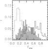Fig. 1 Distributions of disc-to-total mass ratios (Fdisc) estimated by using the gas (solid line), stellar (dashed line) and baryonic (shaded area) mass in simulated galaxies at z = 0. All simulated galaxies have a surviving gaseous disc even in systems where all stars are forming a spheroidal component.

To characterise the morphology of simulated galaxies, we estimated ${\mathit{F}}_{\mathrm{disc}}^{\mathrm{g}}$ (${\mathit{F}}_{\mathrm{disc}}^{\mathrm{\ast }}$) as the mass fraction of the total gas (stellar) mass within 3   R_bar which is supported by rotation (i.e. the D/T ratio for the gas or stellar phase, respectively). We found that, in general, our sample of simulated galaxies is constituted by systems with dominating stellar spheroids and thick stellar discs while the gas mass fractions associated to the spheroid or the disc are very divers. This behaviour can be appreciated more clearly in Fig. 1, where we show the histograms of ${\mathit{F}}_{\mathrm{disc}}^{\mathrm{g}}$ (solid line), ${\mathit{F}}_{\mathrm{disc}}^{\mathrm{\ast }}$ (dashed line) and a similarly defined fraction for the baryonic mass (${\mathit{F}}_{\mathrm{disc}}^{\mathrm{b}}$, shaded area) for simulated galaxies at z = 0³. We can see that the percentage of the stellar mass dominated by rotation does not exceed 60% for any of the analysed galaxies while, for the gas component, we obtained percentages ranging from 20% to  ~100%. When considering the baryonic phase as a whole, the percentage of mass dominated by rotation exhibits an intermediate behaviour with percentages ranging between 10% and 80%. Most of the simulated galaxies in our sample have a significant spheroidal component and all of them have surviving gaseous discs from which it is possible to estimate rotation curves. Our goal here is to analyse if, regardless of galaxy morphology, the gaseous discs can defined a TFR consistent with observations and if the corresponding rotation curves are able to trace the potential wells of their galaxies.

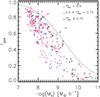Fig. 2 Gas fraction as a function of stellar mass for simulated galaxies. Different symbols depict systems with different values of ${\mathit{F}}_{\mathrm{disc}}^{\mathrm{g}}$, as indicated in the figure. Symbols enclosed by squares correspond to galaxies with ${\mathit{F}}_{\mathrm{disc}}^{\mathrm{b}}\mathrm{\ge }\mathrm{0.5}$. The black dotted curve is the analytical fit to observations given by Stewart et al. (2009) at z = 0.

As shown in Fig. 2, the f_gas of our simulated galaxies decreases with stellar mass, consistently with observations, although at a given stellar mass, they have lower gas fractions than the observed ones (e.g. Stewart et al. 2009; Reyes et al. 2011) as a consequence of the very efficient SN feedback assumed in this model (e.g. de Rossi et al. 2010, 2012). We also appreciate that simulated galaxies with dominant baryonic discs (${\mathit{F}}_{\mathrm{disc}}^{\mathrm{b}}\mathrm{\ge }\mathrm{0.5}$) are biased to lower stellar masses and high gas fractions indicating that the baryonic discs are formed by significant gas masses. In this figure, we also highlighted the simulated galaxies according to the parameter ${\mathit{F}}_{\mathrm{disc}}^{\mathrm{g}}$ (${\mathit{F}}_{\mathrm{disc}}^{\mathrm{g}}\mathit{<}\mathrm{0.5}$, $\mathrm{0.5}\mathrm{\le }{\mathit{F}}_{\mathrm{disc}}^{\mathrm{g}}\mathit{<}\mathrm{0.75}$, ${\mathit{F}}_{\mathrm{disc}}^{\mathrm{g}}\mathrm{\ge }\mathrm{0.5}$) to show the rich variety of gas disc-type galaxies produced by the simulations. While there are no massive stellar galaxies (M_∗ ≳ 10¹⁰   M_⊙   h^-1) with significant stellar disc components, the left-over gas mass is mainly dominated by rotational motions. We have no system dominated by stellar discs, as indicated by the lack of population with ${\mathit{F}}_{\mathrm{disc}}^{\mathrm{g}}\mathit{<}\mathrm{0.5}$ and ${\mathit{F}}_{\mathrm{disc}}^{\mathrm{b}}\mathrm{\ge }\mathrm{0.5}$.

Normal spiral galaxies have aligned gaseous and stellar disc components. Cases of misalignment are generally considered the product of interactions or recent mergers that perturbed the kinematics of the systems (Snaith et al. 2012). Therefore, to gain a clearer picture of the baryonic kinematics in our sample, we calculated the cosines of the angles (α) determined by the angular momenta of the gas discs (J_g) and those of the stellar ones (J_∗). For galaxies with dominant baryonic discs (${\mathit{F}}_{\mathrm{disc}}^{\mathrm{b}}\mathrm{\ge }\mathrm{0.5}$), we estimated these cosines taking into account only the mass associated to the disc component while for systems with dominant baryonic spheroids (${\mathit{F}}_{\mathrm{disc}}^{\mathrm{b}}\mathit{<}\mathrm{0.5}$), we considered the whole baryonic mass. Our results show that cos(α) > 0.95 for all systems with ${\mathit{F}}_{\mathrm{disc}}^{\mathrm{b}}\mathrm{\ge }\mathrm{0.5}$, showing that gaseous and stellar discs are very well aligned, consistent with disc-like galaxies. For galaxies with ${\mathit{F}}_{\mathrm{disc}}^{\mathrm{b}}\mathit{<}\mathrm{0.5}$, J_g and J_∗ are not always aligned, forming angles larger than π/4 in some cases, which reveals different levels of disturbance in the baryonic kinematics. For future discussion, we define three subsamples: S1, constituted by systems with dominant baryonic discs, which are more similar to real spiral galaxies; S2, formed by systems with dominant baryonic spheroids and aligned gas discs (${\mathit{F}}_{\mathrm{disc}}^{\mathrm{b}}\mathit{<}\mathrm{0.5}$ and cos(α) > 0.7); and S3, including galaxies also with dominant baryonic spheroids but misaligned gas discs (${\mathit{F}}_{\mathrm{disc}}^{\mathrm{b}}\mathit{<}\mathrm{0.5}$ and cos(α) ≤ 0.7). The percentages of galaxies corresponding to S1, S2 and S3 are 33%, 31% and 36%, respectively.

Because the main goal of this work is the analysis of the gas kinematics in the disc component, we will characterise simulated systems by using only ${\mathit{F}}_{\mathrm{disc}}^{\mathrm{g}}$ but, when necessary, we will also refer to the subsamples S1, S2 and S3 to obtain a more complete picture. In de Rossi et al. (2010), we restricted our study to galaxies with ${\mathit{F}}_{\mathrm{disc}}^{\mathrm{g}}\mathrm{\ge }\mathrm{0.75}$ so that the gaseous disc components were significant with well-behaved rotation curves. As mentioned before, in this work we extend that analysis to the whole sample of simulated galaxies with a surviving gas disc.

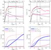Fig. 3 Upper panels: rotation curves for two typical simulated galaxies G1 and G2 (left and right panels, respectively) at z = 0 with different fractions of gas supported by rotation (${\mathit{F}}_{\mathrm{disc}}^{\mathrm{g}}$). The total circular velocity is shown with a solid line. The circular velocities contributed by the gas, stellar, baryonic and dark components are represented with dotted, dot-dashed, dashed and long-dashed lines, respectively. The mean rotation curve (diamonds) and the mean dispersion velocity curve (squares) for the gas-phase are also plotted. The vertical lines indicate the baryonic radius (Rbar) and the radius where the mean rotation velocity reaches a maximum value (Rmax). Lower panels: gas (solid lines) and stellar (dashed lines) mass in the spheroidal (red) and disc (blue) components as a function of radius, normalised to the corresponding total gas or stellar mass within 3   Rbar. The vertical line depicts Rbar.

Fig. 4 Simulated sTFR (upper panels) and bTFR (lower panels) at z = 0 by using Vrot estimated at different radii as indicated in the labels. The green circles depict systems with ${\mathit{F}}_{\mathrm{disc}}^{\mathrm{g}}\mathit{<}\mathrm{0.75}$, while the blue squares represent systems with ${\mathit{F}}_{\mathrm{disc}}^{\mathrm{g}}\mathrm{\ge }\mathrm{0.75}$. The black solid lines indicate the mean relations estimated by using Vcirc measured at the corresponding radii and their standard deviations.

2.2.1. Rotation curves

In the upper panels of Fig. 3, we show the rotation and circular velocities for two typical simulated galaxies at z = 0. The left panels exhibit the results for a galaxy with a stellar mass of M_∗ = 10^9.7   M_⊙   h^-1 and ${\mathit{F}}_{\mathrm{disc}}^{\mathrm{g}}\mathrm{=}\mathrm{0.9}$ (G1), while in the right panels we display those of a galaxy with a stellar mass of M_∗ = 10¹⁰   M_⊙   h^-1 and ${\mathit{F}}_{\mathrm{disc}}^{\mathrm{g}}\mathrm{=}\mathrm{0.6}$ (G2). G1 belongs to the subsample S1 (i.e. systems more similar to real spiral galaxies) and G2 to the subsample S2 (i.e. systems with dominant baryonic spheroids, with aligned gas discs). Evidently, G1 has a more important gas-phase disc component with a rotation curve tracing the circular velocity remarkably well until R_bar, while in the case of G2, it drops at about R_max, departing significantly from the circular velocity. In both cases, the decrease in the rotation curve is accompanied by an increase of the gas mean dispersion velocity, as expected.

In the lower panels of Fig. 3, we can appreciate the gas (solid lines) and stellar (dashed lines) mass fractions associated to the spheroidal (red) and disc (blue) components as a function of radius for G1 and G2. The gas (stellar) mass in each component is normalised to the total gas (stellar) mass enclosed by 3   R_bar. We see that, for G1, the stars are more concentrated than in G2.

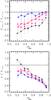Fig. 5 Vrot/Vcirc and σ/Vrot as a function of the fraction of the gas mass supported by rotation and at different radii in the simulations at z = 0: Rmax (dot-dashed line), 0.5   Rbar (solid line), Rbar (dotted line) and 1.5   Rbar (dashed line). Error bars correspond to the standard deviations. It is interesting to note that Vrot at Rmax can approximate Vcirc with good accuracy (>90%) for all simulated systems.

3. The Tully-Fisher relation

The kinematical analysis performed for G1 and G2 in Sect. 2.2 was extended to our whole sample of simulated galactic systems at z = 0. We constructed the sTFR and bTFR by using the rotation velocity and the circular velocity estimated at different radii: R_max, 0.5   R_bar, R_bar and 1.5   R_bar, as shown in Fig. 4. Our simulated TFR agrees very well with that reported by Reyes et al. (2011) over the whole observed mass range ( ≈ 10⁹ − 10¹¹   M_⊙   h^-1). Our SN feedback model is able to reproduce the observed sTFR and bTFR even for these large stellar masses without the need to resort to other physical processes (see McCarthy et al. 2012, for different results). As shown in de Rossi et al. (2010), this SN feedback model can also predict the observed bend of the sTFR at smaller stellar masses M_∗ < 10⁹   M_⊙   h^-1 (e.g. McGaugh et al. 2000; Amorín et al. 2009). Indeed, the good agreement of our simulated TFRs with observations of large and small stellar masses is the result of the action of the self-regulated SN feedback adopted in our models, which is able to regulate the star formation process in systems of different potential wells without the need to introduce ad hoc mass-dependent parameters.

For gaseous disc-dominated systems (blue squares in Fig. 4, ${\mathit{F}}_{\mathrm{disc}}^{\mathrm{g}}\mathrm{\ge }\mathrm{0.75}$, 23% of the total sample), the good agreement between the TFR obtained by using V_rot and that estimated by using V_circ at different radii shows that the former is a good measure of the total potential well. For these systems, we obtained that the scatter in the sTFR and bTFR decreases when V_rot is estimated at  ~0.5   R_bar, in agreement with observations (Yegorova & Salucci 2007). We also found for these systems, that V_rot(R_max) ≈ V_rot(R_bar) consistent with the findings of Persic & Salucci (1995).

For systems with more significant gas spheroidal components (green circles in Fig. 4, ${\mathit{F}}_{\mathrm{disc}}^{\mathrm{g}}\mathit{<}\mathrm{0.75}$), the rotation velocities tend to be lower than the V_circ at a given mass. This is accompanied by the increase in gas velocity dispersion. To quantify the behaviour of the kinematical estimators, in Fig. 5 we show V_rot/V_circ and σ/V_rot as a function of ${\mathit{F}}_{\mathrm{disc}}^{\mathrm{g}}$, measured at different radii (σ is estimated by considering all gas particles within a given radius). When the disc dominates the gas-phase component, V_rot can approximate V_circ with good accuracy (higher than  ~ 90%). However, as ${\mathit{F}}_{\mathrm{disc}}^{\mathrm{g}}$ decreases, V_rot/V_circ becomes lower and σ/V_rot increases as the gas component is increasingly dominated by dispersion, showing stronger variations when measured at larger radii. For galaxies whose gas component is dominated by dispersion (${\mathit{F}}_{\mathrm{disc}}^{\mathrm{g}}\mathit{<}\mathrm{0.4}$), we found a mean value of σ/V_rot ~ 0.7 measured at R_max, in agreement with recent observational results by Catinella et al. (2012).

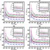Fig. 6 Vi/Vcirc at z = 0 as a function of radius in the simulations for Vi: σ (blue triangles), Vrot (red squares), s0.5 (black crosses), s1.0 (green asterisks) and S (pink diamonds). Each symbol represents the averaged value over the entire sample of galaxies (upper left panel) and the subsamples S1, S2 and S3 defined in Sect. 2.2 (upper right panel, lower left panel and lower right panel, respectively). The corresponding standard deviations are also shown. The radii are given normalised to Rbar in the main panels while in the insets, they are given normalised to Rmax. The horizontal solid line indicates where Vi agrees with Vcirc, while the dashed horizontal lines denote the range where Vi does not depart more than 20% from Vcirc.

We recalculated these trends for the subsamples S1, S2 and S3 (see Sect. 2.2), obtaining similar global results. For σ/V_rot, regardless of the alignment between stellar and gaseous angular momenta, galaxies with dominating baryonic spheroids have also more highly disturbed gas dynamics, implying higher ratios than those for systems with a baryonic dominating disc at a given ${\mathit{F}}_{\mathrm{disc}}^{\mathrm{g}}$.

As we note from Fig. 5, a very interesting result from our model is that V_rot at R_max seems to be the best proxy for the circular velocity because it shows no significant dependence on ${\mathit{F}}_{\mathrm{disc}}^{\mathrm{g}}$: V_rot is always within 90% of V_circ for all systems. This trend is even better for gas systems dominated by rotation. We checked these trends for S1, S2 and S3, finding similar results. Regardless of the relative angular momentum orientation between stellar and gas components, V_rot at R_max provides on average the best indicator for the total circular velocity, although with high standard deviations for systems with ${\mathit{F}}_{\mathrm{disc}}^{\mathrm{b}}\lesssim \mathrm{0.5}$.

As discussed in the introduction, Kassin et al. (2007) and Covington et al. (2010) proposed new kinematical estimators based on observational and numerical results, respectively, to account for the disordered motions in the gas component with the aim at explaining the origin of the scatter in the TFR. We tested these estimators in our cosmological simulations. In Fig. 6, we can appreciate V_i/V_circ at z = 0 as a function of radius where V_i could be either σ, V_rot, s_0.5, s_1.0 or S. Each symbol represents the averaged value over the entire sample of galaxies (upper left panel) and the subsamples S1, S2 and S3 defined in Sect. 2.2 (upper right panel, lower left panel and lower right panel, respectively). The corresponding standard deviations are also shown. The radii are given normalised to R_bar in the main panels while in the insets, they are given normalised to R_max. The horizontal solid line indicates where V_i agrees with V_circ, while the dashed horizontal lines denote the range where V_i does not depart more than 20% from V_circ. By analysing the main panels of this figure it is clear that σ is lower than V_circ at almost all analysed radii with the only exception of the inner parts of the galaxies. At radii larger than 0.5   R_bar, σ/V_circ remains almost constant at  ≈ 0.55 if we consider the whole sample of galaxies,  ≈0.50 in the case of S1 and  ≈ 0.60 for S2 and S3. These findings are consistent with the fact that S1 is comprised of more disc-like galaxies and hence, the dispersion velocities tend to be lower. For the whole galaxy sample, our results indicate that V_rot can be considered a proxy for V_circ in the range 0.2   R_bar < r < 0.5   R_bar. Similar trends can be appreciated for the subsamples S2 and S3 but in the case of S1, this range can be extended towards 0.7   R_bar, approximately. By comparing V_circ with s_0.5 and S, we see that the former underestimates V_circ, while the latter overproduces it for the whole sample and for S1, S2 and S3. Nevertheless, in the case of S1, S constitutes a better representation of V_circ as a consequence of the lower dispersion velocities in this subsample. The analysis of the rotation and dispersion velocity curves of our simulated galaxies suggests that the best proxy for V_circ at z = 0 is s_1.0, which approximates the simulated V_circ remarkably well at r > 0.5   R_bar for our whole sample and each one of the subsamples.

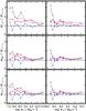Fig. 7 Ratio between the standard deviations of Vi and Vcirc (ΔVi/ΔVcirc) at z = 0 for different bins of stellar (M∗) and baryonic (Mb) mass. Each bin is constituted by 35 galaxies of similar stellar or baryonic masses. Results are shown for Vi: Vrot (upper panels), s0.5 (middle panels) and s1.0 (lower panels). The kinematical indicators are estimated by evaluating the gas kinematics at different radii in the simulations: Rmax (dot-dashed line), 0.5   Rbar (solid line), Rbar (dotted line) and 1.5   Rbar (dashed line).

When analysing the behaviour of V_i/V_circ as a function of R/R_max (insets of Fig. 6), we note that for the whole sample of galaxies the scatter in the vertical axis increases significantly, mainly at R/R_max ~ 1. We can see that the main contribution to this scatter comes from galaxies in S2 and S3, while in the case of S1 the scatter is quite small. For S3, the scatter is even larger than for S2 because these systems exhibit a more highly disturbed baryonic kinematics (misaligned gas discs). It is interesting to note that in these simulations, the rotation curves of spheroid-dominated systems tend to be more affected in the inner parts of the galaxy (R ~ R_max) than outwards (R ~ R_bar). It is also worth noting that for the three subsamples, on average, V_rot ≈ V_circ at R ~ R_max.

In Fig. 7, we plotted the ratio between the standard deviation of the TFR by using V_rot, s_0.5 and s_1.0 and the standard deviation by using V_circ. The ratio is analysed as a function of stellar and baryonic mass. We can appreciate that by combining V_rot and σ in the definition of the kinematical indicator s_0.5 or s_1.0, the dispersion in the sTFR and bTFR at a given mass is considerably reduced. By analysing these trends for S1, S2 and S3 separately, we found that this scatter is mostly generated by galaxies in S2 and S3 (but mainly in S3) given the lower mass fractions associated to their surviving discs. Nevertheless, all kinematical indicators including V_rot lead to the tightest relation if evaluated at R_max. Hence, V_rot at R_max not only seems to be a very good representation of the potential well of simulated systems, regardless of the morphology (Figs. 5, 6) but the scatter of the sTFR and bTFR also tends to be reduced if the velocity indicators are evaluated at this radius. This may be suggesting that R_max can be considered a characteristic radius for the gas kinematics of galaxies, at least for the potential wells reproduced by these simulations. From Fig. 7, we also appreciate that both s_0.5 and s_1.0 reduce the scatter of the TFR by similar amounts but in the literature, most authors use s_0.5. In our simulations we found s_1.0 to be a better tracer of the gas kinematics because it is also a good proxy for V_circ (Fig. 6). Finally, by comparing the relative deviations of the sTRF and bTFR (left- and right-hand panels of Fig. 7), it is evident that the bTFR is tighter than the sTFR for the analysed mass range everywhere but at the lowest masses. The less massive systems are also the most affected by numerical resolution, therefore the trends at the low-mass end should be confirmed with higher numerical resolution simulations.

4. The effects of galaxy assembly in the TFR-plane

To understand the evolution of the gas kinematics in simulated galaxies and its implications for the origin of the scatter in the sTFR and bTFR, we analysed the evolution of galaxies on the TFR-plane as a function of time and in relation to important events such as mergers. To accomplish this purpose, we reconstructed the assembly history of the complete sample of simulated galaxies from their formation time to z = 0 and explored which events disturb their rotation curves and lead to outliers on the TFR-plane. We designed our own algorithm to follow the main progenitor branch for each simulated galaxy. At each available time, we define the main progenitor as the most massive baryonic substructure. All other smaller systems in the tree are considered satellites that will eventually merge onto the main branch.

Fig. 8 Formation histories for six typical simulated galaxies at z = 0 in the simulations, with different stellar (M∗) and baryonic (Mb) masses and circular velocities (Vcirc). The masses are given in logarithm and in units of M⊙   h-1. The circular velocities are given in logarithm and in units of km   s-1. In each panel, we show the evolution of ${\mathit{F}}_{\mathrm{inter}}^{{\mathit{R}}_{\mathrm{vir}}}$ (dotted line) and ${\mathit{F}}_{\mathrm{inter}}^{\mathrm{2}{\mathit{R}}_{\mathrm{vir}}}$ (dashed line) in box A. In box B, we can appreciate Fmerger. Box C shows the time evolution of the gas fraction (dotted line), baryonic mass relative to the final one (triple-dot-dashed line) and ${\mathit{F}}_{\mathrm{disc}}^{\mathrm{g}}$ (dashed line). Box D shows the star formation efficiency SFRe in yr-1 and, in box E, we can appreciate the ratio Vrot/Vcirc (dashed lines) and s1.0/Vcirc (solid lines) evaluated at Rbar. See text for definitions of variables.

To evaluate the effects of the galaxy-galaxy interactions, we determined the total mass within R_bar (${\mathit{M}}_{\mathrm{dyn}}^{\mathrm{main}}$) for a given galaxy and the mass of all its neighbours (${\mathit{M}}_{\mathrm{dyn}}^{\mathrm{neighb}}$) located at a distance shorter than a certain radius D, which can be taken either as the virial radius (R_vir) or as twice its value. We quantified the strength of interactions by the ratio ${\mathit{F}}_{\mathrm{inter}}^{\mathit{D}}\mathrm{=}\sum {\mathit{M}}_{\mathrm{dyn}}^{\mathrm{neighb}}\mathit{/}{\mathit{M}}_{\mathrm{dyn}}^{\mathrm{main}}$. This ratio is measured at both distances to form an idea of the satellite distribution with respect to the main progenitor (for example if most of them are within R_vir or farther away). To quantify the strength of mergers, the ratio 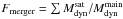${\mathit{F}}_{\mathrm{merger}}\mathrm{=}\sum {\mathit{M}}_{\mathrm{dyn}}^{\mathrm{sat}}\mathit{/}{\mathit{M}}_{\mathrm{dyn}}^{\mathrm{main}}$ is defined, where ${\mathit{M}}_{\mathrm{dyn}}^{\mathrm{sat}}$ is the mass of the satellites that were accreted between two available times.

For the main progenitor, we estimated the gas fraction, its baryonic mass normalised to the value at z = 0 and ${\mathit{F}}_{\mathrm{disc}}^{\mathrm{g}}$ as a function of lookback time to quantify the building-up of the galaxy as well as the role of outflows, as we will discuss in next section. We also calculated the star formation rate efficiency (SFRe) in the progenitor galaxy as the ratio between the star formation rate and the gas mass. We will use the ratios V_rot/V_circ and s_1.0/V_circ to quantify the disturbance of the rotation curve along the evolutionary paths. All these quantities are estimated at R_bar.

4.1. Formation histories of typical galaxies

We analysed the evolution of the quantities defined above for the main progenitor branch of the local simulated galaxies as a function of lookback time. To illustrate the relation between interactions and mergers and disturbances of the rotation curve, we selected six typical galaxies out of a sample of 309 galaxies at z = 0, as shown in Fig. 8.

The galaxy in the upper-left panel of Fig. 8 is one of the more massive galaxies at z = 0, exhibiting a lower scatter in the local simulated TFR. As expected, V_rot/V_circ is approximately 1 at z ~ 0 while s_1.0/V_circ tends to be slightly higher by  ~0.1 dex. By analysing its formation history, we see that the main progenitor has not experienced significant interactions or merger events during the last 5 Gyr. Its SFRe has also decreased by more than an order of magnitude in the same time interval as a consequence of the decrease of the gas fraction. Therefore, the galaxy at z = 0 has reached a passive stage of evolution and stability, which is consistent with its well-defined rotation curve and low scatter in the TFR. Note also that although the gas fraction is small (~0.07) at z = 0, the gas mass within R_bar is  ≈ 3 × 10⁹   M_⊙   h^-1 so that it is possible to have a well-resolved disc component. By exploring the main progenitor branch at early times, we can see that for a lookback time longer than 8 Gyr the main progenitor exhibited a disturbed kinematics. At this epoch, the ratio V_rot/V_circ shows variations by  ± 0.1 dex over time intervals of about 1 Gyr. From the inspection of F_inter and F_merger at that time, we can infer that this behaviour can be associated with interaction and merger events that led to a high SFRe and exhausted the gas reservoir of the system. It is interesting that merger and interactions can generate either an increase or decrease of V_rot/V_circ (Pedrosa et al. 2008). With respect to s_1.0/V_circ, we obtained similar trends but with smaller and smoother variations.

The galaxy in the upper right panel is an example of an intermediate-mass galaxy with low scatter in the local TFR. This galaxy also exhibits a passive evolution within the last few Gyr. Similarly to the previous example, we can see that at early times (~9 Gyr ago), its main progenitor experienced significant interactions followed by merger events (${\mathit{F}}_{\mathrm{inter}}^{\mathrm{2}{\mathit{R}}_{\mathrm{vir}}}\mathrm{~}\mathrm{0.4}$, ${\mathit{F}}_{\mathrm{inter}}^{{\mathit{R}}_{\mathrm{vir}}}\mathrm{~}\mathrm{0.3}$, F_merger ~ 0.25) that could be linked to a decrease in V_rot/V_circ ratio by around  ~ 0.5 dex over the corresponding period. Note also that ${\mathit{F}}_{\mathrm{disc}}^{\mathrm{g}}$ exhibits a minimum at that epoch. After these events, its disc component was reconstructed and the gas rotation velocity approached the circular velocity again. It is worth noting that s_1.0/V_circ ~ 1 during the whole formation history of this galaxy, even during the epoch of mergers and interactions. As previously reported in the literature, these findings suggest that the combination of V_rot and σ in the definition of the kinematical indicator generates a velocity scale more robust against disturbances of the gas kinematics.

In the middle panels of Fig. 8, we compare the formation histories of two smaller galaxies with similar stellar masses of M_∗ ≈ 10^9.4   M_⊙   h^-1 and circular velocities of V_circ ≈ 100  km   s^-1. The galaxy in the left panel exhibits a smaller scatter in the local TFR than the galaxy in the right one. By comparing the recent formation histories of these galaxies, we see that the large scatter in the second one can be associated to strong interactions (${\mathit{F}}_{\mathrm{inter}}^{\mathrm{2}{\mathit{R}}_{\mathrm{vir}}}\mathrm{~}\mathrm{0.4}$ and ${\mathit{F}}_{\mathrm{inter}}^{{\mathit{R}}_{\mathrm{vir}}}\mathrm{~}\mathrm{0.2}$) taking place during the last 6 Gyr that culminated in a recent important merger event (F_merger ~ 0.25). Before this epoch, the V_rot/V_circ for the main progenitor remains close to  ~ 1. In the case of s_1.0/V_circ, the behaviour is similar but with smoother variations. Simultaneously with the interactions and merger events, the gas fraction increases and the percentage of gas in the disc component decreases, indicating the presence of gas inflows that contribute more importantly to the formation of a spheroidal component. In the galaxy in the left panel, the lack of mergers and interactions during the last 5 Gyr agrees with the small variations of V_rot/V_circ and the high values of ${\mathit{F}}_{\mathrm{disc}}^{\mathrm{g}}$. However, its main progenitor experiences an increase of V_rot/V_circ 7 Gyr ago, during a merger event (F_merger ~ 0.15), while 9 Gyr ago, a strong interaction (${\mathit{F}}_{\mathrm{inter}}^{\mathrm{2}{\mathit{R}}_{\mathrm{vir}}}\mathrm{~}\mathrm{0.6}$) can be linked to a decrease by more than 0.1 dex in V_rot/V_circ. Once again, the trends for s_1.0/V_circ are similar to those appreciated for V_rot/V_circ but with a smoother evolution. As seen before, ${\mathit{F}}_{\mathrm{disc}}^{\mathrm{g}}$ reaches a minimum during the period of strong interactions.

Finally, in the lower panels, we compare the evolution of galaxies with low stellar masses of M_∗ ≈ 10^8.4   M_⊙   h^-1 and circular velocities of V_circ ≈ 50  km   s^-1. The galaxy in the left panel shows a smaller scatter in the local TFR than the one in the right panel. Even in these small galactic systems, the scatter in V_rot/V_circ seems to be related to the presence of merger events. The galaxy in the left panel has not suffered significant mergers or interactions during the last 5 Gyr, in agreement with its small changes of V_rot/V_circ. However, the progenitor in the main branch has been affected by mergers and interactions 8 Gyr ago, which led to a peak in the SFRe and caused changes by  ~ 0.25 dex in V_rot/V_circ and  < 0.15 dex in the case of s_1.0/V_circ. For the galaxy in the right panel, the distortion of the rotation curve at z ~ 0 can be again related to recent significant mergers and interactions: ${\mathit{F}}_{\mathrm{inter}}^{{\mathit{R}}_{\mathrm{vir}}}\mathrm{~}\mathrm{0.3}$ and F_merger ~ 0.3.

Therefore, our results suggest that the hierarchical aggregation of the structure strongly influences the evolution of the galactic gas component within a Λ-CDM Universe, producing TFR outliers in concordance with previous works (e.g. Simard & Pritchet 1998; Barton et al. 2001; Kannappan & Barton 2004; Böhm et al. 2004; Flores et al. 2006; Weiner et al. 2006; Kassin et al. 2007). Mergers and interactions seem to be important for regulating the gas kinematics and star formation process for the whole range of stellar masses covered by these simulations, affecting the evolutionary tracks of systems on the TFR-plane. All these phenomena seem to be responsible for the scatter we found in the TFR. As previously reported in the literature (e.g. Kassin et al. 2007), we obtained that the combination of V_rot and σ leads to a velocity scale more stable during merger and interaction events reducing the scatter in the sTFR and bTFR. We obtained, for example, that  | log (V_rot/V_circ) |  < 0.5 for the whole sample of simulated systems while  | log (s_1.0/V_circ) |  < 0.3. However, some observational works reported scatters in the sTFR greater than  ~1 dex (e.g. Kassin et al. 2007). In this context, it is worth mentioning that the dispersion in the observed TFR relation might depend very sensitively on the observational approach and modelling techniques (e.g. Miller et al. 2011) and it is not yet clear which is the intrinsic scatter of the relation. By analysing numerical simulations, Covington et al. (2010) found scatters larger than 1 dex. Nevertheless, those simulations were pre-prepared mergers of two isolated galaxies. In this work, by studying cosmological simulations, we are able to follow the evolutionary history of galaxies in a self-consistent way.

4.2. Fingerprints of formation histories on the TFR-plane

In this section, we investigate how the assembly histories of galaxies in a cosmological scenario induced changes in the TFR-plane by searching for fingerprints of particular events which, then, can be used to understand observations.

In Fig. 9, we can appreciate the evolution on the sTFR and bTFR planes of the six galaxies described in the previous section. If the TFR is constructed by using V_circ, it provides us with information about how the stellar and baryonic masses assembled within the potential well of the dark haloes hosting the galaxies, while if V_rot is used, it gives information related to the gas kinematics. To assess when galaxies are outliers of the mean TFR at different redshift, we also included the mean sTFR and bTFR of the whole population as a function of redshift taken from de Rossi et al. (2010). For the sake of clarity, we did not include the tracks given by s_1.0 in Fig. 9 but they can be easily derived from previous section: s_1.0 would in general lead to similar trends as those obtained from V_rot but with a less noisier evolution and, given that s_1.0 is higher than V_rot by definition, the tracks would be also displaced towards higher velocities.

By comparing Figs. 8 and 9, we can understand the origin of the changes as the systems evolve. In particular, we see that mergers lead to an increase of V_circ and mass in different amounts. With respect to interactions, in some cases, we detect a decrease in V_circ due to interactions while in others the interaction generates an increase of the stellar and baryonic mass with an almost constant V_circ. When following the TFR tracks using V_rot, we found a very noisy evolution that is considerably affected by interactions and mergers that produce outliers of the TFR. As expected, we see in Fig. 9 that the tracks given by V_circ are smoother than those given by V_rot. Most mergers and interactions generate a scatter in the TFR greater than the level of evolution that we estimated since z = 3 for the relation based on V_circ in these simulations. As we noted before, these events can shift the V_rot towards lower or higher values than V_circ. These findings suggest that from the observational point of view, selection effects and noise are likely to mask the actual evolution of the TFR.

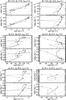Fig. 9 Evolutionary tracks of the six galaxies shown in Fig. 8 on the sTFR and bTFR planes. The background grey lines depict the mean sTFR and bTFR obtained by using Vcirc at Rbar as a kinematical indicator at z = 3,2,1,0.4,0 (dotted, dashed, dot-dashed, triple-dot-dashed, solid line, respectively). The black lines indicate the track of the given galaxy on the TFR plane by using Vcirc (solid line) and Vrot (dashed line) at Rbar as the kinematical indicators. In each panel, there is an arrow indicating in which direction the galaxy evolves along each path.

For the galaxy corresponding to the upper left panel, the most important evolution in the TFR-plane took place more than 8 Gyr ago, during an epoch of important interactions and mergers (${\mathit{F}}_{\mathrm{inter}}^{\mathrm{2}{\mathit{R}}_{\mathrm{vir}}}\mathrm{~}\mathrm{4}$, F_merger ~ 0.3) that generated an increase by more than 1.5 dex in stellar and baryonic mass and by  ~0.4 dex in circular velocity.

For the galaxy in the upper right panel, the track given by V_rot approximates the one given by V_circ with the only exception of the point associated to a lookback time of  ~9 Gyr when the system experienced a significant merger event (F_merger ~ 0.25). As a consequence of the merger, V_rot decreased by  ~0.4 dex departing from V_circ and generating a TFR outlier. After  ~1 Gyr, the disc component was reconstructed, with V_rot approaching V_circ.

With respect to the galaxies in the middle panels, we see that the evolutionary tracks given by V_rot are noisier than those of more massive galaxies. This suggests that interactions and mergers in these simulations are more efficient at producing instabilities in the disc component of systems with shallower potential wells. In these galaxies, the variations in the rotation velocity between two time steps of the simulation are, in some cases, larger that the total level of evolution of the TFR based in V_circ for 3 < z < 0. In particular, the galaxy in the middle right panel reaches z ~ 0 as an outlier of the TFR as a consequence of recent important interactions followed by a merger event (${\mathit{F}}_{\mathrm{inter}}^{\mathrm{2}{\mathit{R}}_{\mathrm{vir}}}\mathrm{~}\mathrm{0.4}$, ${\mathit{F}}_{\mathrm{inter}}^{{\mathit{R}}_{\mathrm{vir}}}\mathrm{~}\mathrm{0.2}$, F_merger ~ 0.25). In this figure, it is evident that during mergers and interactions the tracks given by V_circ and V_rot may diverge.

In the lower panels of Fig. 9, we can appreciate that low-mass galaxies also show a similar behaviour. The galaxy in the left panel becomes an outlier of the TFR given by V_rot at a lookback time of  ~9 Gyr due to interactions and mergers. After  ~1 Gyr, this galaxy recovered its rotational equilibrium with V_rot approaching V_circ again. In the case of the young galaxy in the right panel, the presence of mergers and interactions displaced this galaxy away from the mean TFR based in V_circ. We can also appreciate that due to a recent merger event, V_circ and V_rot evolve in opposite ways.

Although we have pointed out only the correlation between mergers and interactions, we know from the previous section that outflows and inflows can also be associated to sharp changes on the TFR-plane. However, in most cases they also occurred close to mergers or interactions as a second-order effect because these violent events have been proven to be efficient at triggering gas inflows and starbursts (which can drive outflows, e.g. Barnes & Hernquist 1996; Mihos & Hernquist 1996; Tissera 2000).

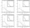Fig. 10 Distribution of the absolute variation of log (Vrot/Vcirc) (main panels) and log (s1.0/Vcirc) (insets) during the last 2 Gyr of evolution for galaxies that have been subject to extreme processes (dashed lines): Fmerger > 0.3 (upper left panel), ${\mathit{F}}_{\mathrm{inter}}^{{\mathit{R}}_{\mathrm{vir}}}\mathit{>}\mathrm{0.6}$ (upper right panel), ΔMbar/Mbar <  − 0.3 (lower left panel) and Δfgas > 0.3 (lower right panel). Solid lines show the corresponding distributions for the whole sample of simulated galaxies at available redshifts.

4.3. Statistical analysis

Our results for these six galaxies suggest that the hierarchical building-up of the structure strongly influences the evolutionary paths of galaxies in the TFR-plane, modulating the evolution of its scatter with cosmic time. To generalise these findings, we performed a statistical study by extending the previous analysis to the whole sample of simulated galaxies. Within the hierarchical aggregation paradigm, galaxies are affected by different types of physical processes such as mergers, interactions, star formation, outflows, gas accretions, etc. All these processes act together to drive galaxy evolution and hence it is not easy to distinguish the effect of each individual event on the variation of the properties of galaxies. It is also possible that the combined actions of two or more different astrophysical processes compensate each other to generate an insignificant change of the mean properties of the system. Therefore, we decided to focus our attention on galaxies that have experienced extreme physical events in the very recent past (in the previous 2 Gyr of galaxies selected at a given z). For these cases, we expect the evolution of the mean properties of galaxies to be mainly affected by a particular extreme physical event.

We assumed that a galaxy has experienced an extreme event when one of the following conditions is true: F_merger > 0.3 (Fig. 10, upper left panel), ${\mathit{F}}_{\mathrm{inter}}^{{\mathit{R}}_{\mathrm{vir}}}\mathit{>}\mathrm{0.6}$ (Fig. 10, upper right panel), ΔM_bar/M_bar <  −0.3 (Fig. 10, lower left panel) and Δf_gas > 0.3 (Fig. 10, lower right panel). ΔM_bar/M_bar is defined as the change in the baryonic mass of the galaxy between two time steps of the simulation if the time interval is not longer than 2 Gyr and is normalised to the initial baryonic mass. In these simulations, a decrease in the baryonic mass of a galaxy (ΔM_bar/M_bar < 0) implies a significant loss of gas and, therefore, the condition ΔM_bar/M_bar <  −0.3 allows us to select systems that have been subject to strong outflows events. Indeed, these simulated galaxies would have lost at least 30% of their baryonic mass during the last 2 Gyr. Δf_gas is defined as the total variation in the gas fraction of the galaxy with time. In these simulations, the gas inside the galaxy tends to decrease because of the star formation process or ejections by galactic winds. Hence, the gas mass can only increase by infall of surrounding material and/or by mergers. Therefore, our condition Δf_gas > 0.3 allows us to identify galactic systems that have suffered substantial gas accretion.

We estimated the distribution of the absolute variations of log (V_rot/V_circ) and log (s_1.0/V_circ) of galaxies that have suffered extreme events, as shown in Fig. 10. For comparison, we calculated the corresponding distribution for the whole sample of simulated galaxies. From the histograms, it is clear that the distribution of galaxies that have been subject to extreme events are biased to higher values of  | Δlog (V_rot/V_circ) |  than those of the whole galaxy sample, indicating that all these processes tend to generate TFR outliers by disturbing the gas kinematics. In particular, most events (from any of the mechanisms considered) induce mean deviations of  ~ 0.1 dex, with maximum offsets in the range [0.4, 0.5] dex. We can also see that  | Δlog (V_rot/V_circ) |  < 0.5 but if we use s_1.0 instead of V_rot, the distribution is narrower with  | Δlog (s_1.0/V_circ) |  < 0.3, approximately. In the case of  | Δlog (s_1.0/V_circ) | , disturbed galaxies tend to be biased towards higher values when associated to mergers and interactions. However, the deviations of s_1.0 from V_circ are less significant in the case of strong inflows and outflows. This suggests that s_1.0 can account better for dispersion associated to these effects than to those that could be imprinted by more violent effects such as mergers and interactions.

To analyse if there is any trend for some of the mechanisms to drive a positive or negative variation of the rotation velocity relative to the circular one, we estimated the percentage of galaxies with Δlog (V_rot/V_circ) < 0 in each of the subsamples. We found a weak trend for galaxies experiencing important mergers or outflows to have negative variations (61% and 58%, respectively) while strong interactions and gas inflows can drive either positive or negative outliers on the TFR-plane (49% and 53%, respectively).

These results indicate that the joint action of mergers, interactions, starbursts, outflows and gas accretion can affect the TFR producing variations in log (V_rot/V_circ) as large as  ~0.5 dex, at least in these simulations. Hence, at a given stellar or baryonic mass, these events can produce a scatter in the TFR-plane larger than the mean level of velocity evolution since z ~ 3 (~0.1 dex). Indeed, for any of the subsamples analysed in Fig. 10, while  ~25% of the galaxies have variations in log (V_rot/V_circ) of  ~0.1 dex, 55% of the systems exhibit values  > 0.1 dex, which might mask the evolution of the TFR in observational studies. However, as we have seen, by combining V_rot and σ in the definition of the kinematical indicator, it is possible to generate a velocity scale more robust against disturbances of the gas kinematics, which is able to reduce the scatter in the simulated sTFR and bTFR by a factor of  ~2.

5. Conclusions

We studied the evolution of the gas kinematics of galaxies with numerical simulations that include a physically motivated SN feedback. We focused on the origin of the scatter of galaxies in the TFR-plane and the connection with the formation histories of these systems. In particular, we analysed the role of mergers and interactions on the determination of gas kinematics and of the features of rotation curves during the assembly of galaxies. We extended the work by de Rossi et al. (2010), who studied gas rotation-dominated systems, and explored the whole sample of galactic systems, including also gas dispersion-dominated galaxies. It is worth mentioning that our simulated sample does not contain realistic spiral-like galaxies as, in general, simulated systems have dominant stellar spheroids. Nevertheless, all analysed galaxies have surviving gaseous discs, which are found to be good tracers of the potential wells.

Our main results can be summarised as follows:

• Our simulations support the claim that V_rot is the best proxy for V_circ at R_max for galaxies of all morphology types. For gas rotation-dominated systems, V_rot is a good proxy of V_circ at all radii. As the dispersion-dominated component increases, σ/V_rot increases, particularly in the outer parts of the systems. This leads to an increase of the scatter of the TFR when considering systems with more disordered gas kinematics. Nevertheless, for systems with large dispersion-dominated components, V_rot is still a good proxy for V_circ at R_max. In particular, for spheroidal dominated galaxies, we obtained a mean σ/V_rot of  ~0.7 at R_max in good agreement with recent observations (Catinella et al. 2012).

• The use of the kinematical indicators s_0.5, s_1.0 and S (Weiner et al. 2006; Kassin et al. 2007; Covington et al. 2010) in our galaxy sample led to a reduction of the scatter of the TFR in all cases. Moreover, all of them, together with V_rot, led to the tightest relations if evaluated at R_max. In particular, by comparing s_0.5 and S with V_circ, we obtained that the former underestimates V_circ, while the latter overproduces it. Although in the literature s_0.5 has been used more frequently, we find that for our simulations, s_1.0 is a better kinematical indicator because it does not only reduce the scatter of the TFR but it is also a good proxy of V_circ at large radii (r > 0.5   R_bar). By restricting our study to subsamples with different baryonic D/T or different relative angular momentum orientation between the gas and stellar phases, we obtained, on average, similar global trends. Nevertheless, galaxies with misalignments between the gaseous and the stellar angular momenta or with lower baryonic D/T present larger scatter around the mean behaviour.

• Mergers and interactions within a Λ-CDM scenario can regulate the star formation process as well as drive inflows and outflows of gas affecting the evolutionary tracks of galaxies on the TFR-plane and generating TFR outliers. In particular, we obtained that merger-induced velocity disturbances in our cosmological simulations are typically smaller (<0.5 dex) than predicted by pre-prepared merger simulations of Milky-Way type galaxies (Covington et al. 2010). This is a consequence of the fact that the cosmological merger histories of the galaxies in the simulated mass range involved typically more minor mergers than the major mergers commonly built in merger simulations.

• We detected that mergers and interactions can generate either an increase or decrease of V_rot/V_circ. Nevertheless, statistically, we obtained a weak trend for galaxies subject to important mergers to be biased to negative variations (~61%), while strong interactions can generate either positive or negative changes with similar probability. We also found that gas infall or outflows can lead to TFR outliers. In particular, the statistical study shows a weak trend for outflows to produce negative variations (~58%) while gas inflows can drive either positive or negative changes.

• By comparing the distributions of the absolute variations of log (s_1.0/V_circ) and log (V_rot/V_circ) during the evolution of all simulated galaxies, we obtained that for the former case, the scatter is reduced by a factor of  ~2, exhibiting a narrower distribution ( | Δlog (s_1.0/V_circ) |  < 0.3). In particular, mergers and interactions can be associated to a larger scatter in the TFR even when using s_1.0; conversely, the effects of inflows and outflows seem to be more efficiently accounted for by this kinematical indicator.

• According to our results, extreme physical events in simulated galaxies (e.g. mergers, interactions, outflows and inflows) lead to a scatter on the TFR-plane larger than the mean level of evolution of the TFR since z ~ 3. In addition, by enhancing the star formation rate, mergers and interactions also affect the luminosity and M/L ratio of the systems, which can induce observational offsets from the TFR. Therefore, much work is still needed from the observational and theoretical point of views to address these problems.

Acknowledgments

We thank the anonymous referee for his/her useful comments that helped significantly to improve this paper. We thank Mario Abadi for useful comments. We acknowledge support from the PICT 32342 (2005), PICT 245-Max Planck (2006) of ANCyT (Argentina), PIP 2009-112-200901-00305 of CONICET (Argentina) and the L’oreal-Unesco-Conicet 2010 Prize. Simulations were run in Fenix and HOPE clusters at IAFE.

References

All Figures

	Fig. 1 Distributions of disc-to-total mass ratios (Fdisc) estimated by using the gas (solid line), stellar (dashed line) and baryonic (shaded area) mass in simulated galaxies at z = 0. All simulated galaxies have a surviving gaseous disc even in systems where all stars are forming a spheroidal component.
In the text

Fig. 2 Gas fraction as a function of stellar mass for simulated galaxies. Different symbols depict systems with different values of ${\mathit{F}}_{\mathrm{disc}}^{\mathrm{g}}$, as indicated in the figure. Symbols enclosed by squares correspond to galaxies with ${\mathit{F}}_{\mathrm{disc}}^{\mathrm{b}}\mathrm{\ge }\mathrm{0.5}$. The black dotted curve is the analytical fit to observations given by Stewart et al. (2009) at z = 0.

In the text

Fig. 3 Upper panels: rotation curves for two typical simulated galaxies G1 and G2 (left and right panels, respectively) at z = 0 with different fractions of gas supported by rotation (${\mathit{F}}_{\mathrm{disc}}^{\mathrm{g}}$). The total circular velocity is shown with a solid line. The circular velocities contributed by the gas, stellar, baryonic and dark components are represented with dotted, dot-dashed, dashed and long-dashed lines, respectively. The mean rotation curve (diamonds) and the mean dispersion velocity curve (squares) for the gas-phase are also plotted. The vertical lines indicate the baryonic radius (Rbar) and the radius where the mean rotation velocity reaches a maximum value (Rmax). Lower panels: gas (solid lines) and stellar (dashed lines) mass in the spheroidal (red) and disc (blue) components as a function of radius, normalised to the corresponding total gas or stellar mass within 3   Rbar. The vertical line depicts Rbar.

In the text

Fig. 4 Simulated sTFR (upper panels) and bTFR (lower panels) at z = 0 by using Vrot estimated at different radii as indicated in the labels. The green circles depict systems with ${\mathit{F}}_{\mathrm{disc}}^{\mathrm{g}}\mathit{<}\mathrm{0.75}$, while the blue squares represent systems with ${\mathit{F}}_{\mathrm{disc}}^{\mathrm{g}}\mathrm{\ge }\mathrm{0.75}$. The black solid lines indicate the mean relations estimated by using Vcirc measured at the corresponding radii and their standard deviations.

In the text

Fig. 5 Vrot/Vcirc and σ/Vrot as a function of the fraction of the gas mass supported by rotation and at different radii in the simulations at z = 0: Rmax (dot-dashed line), 0.5   Rbar (solid line), Rbar (dotted line) and 1.5   Rbar (dashed line). Error bars correspond to the standard deviations. It is interesting to note that Vrot at Rmax can approximate Vcirc with good accuracy (>90%) for all simulated systems.

In the text

Fig. 6 Vi/Vcirc at z = 0 as a function of radius in the simulations for Vi: σ (blue triangles), Vrot (red squares), s0.5 (black crosses), s1.0 (green asterisks) and S (pink diamonds). Each symbol represents the averaged value over the entire sample of galaxies (upper left panel) and the subsamples S1, S2 and S3 defined in Sect. 2.2 (upper right panel, lower left panel and lower right panel, respectively). The corresponding standard deviations are also shown. The radii are given normalised to Rbar in the main panels while in the insets, they are given normalised to Rmax. The horizontal solid line indicates where Vi agrees with Vcirc, while the dashed horizontal lines denote the range where Vi does not depart more than 20% from Vcirc.

In the text

Fig. 7 Ratio between the standard deviations of Vi and Vcirc (ΔVi/ΔVcirc) at z = 0 for different bins of stellar (M∗) and baryonic (Mb) mass. Each bin is constituted by 35 galaxies of similar stellar or baryonic masses. Results are shown for Vi: Vrot (upper panels), s0.5 (middle panels) and s1.0 (lower panels). The kinematical indicators are estimated by evaluating the gas kinematics at different radii in the simulations: Rmax (dot-dashed line), 0.5   Rbar (solid line), Rbar (dotted line) and 1.5   Rbar (dashed line).

In the text

Fig. 8 Formation histories for six typical simulated galaxies at z = 0 in the simulations, with different stellar (M∗) and baryonic (Mb) masses and circular velocities (Vcirc). The masses are given in logarithm and in units of M⊙   h-1. The circular velocities are given in logarithm and in units of km   s-1. In each panel, we show the evolution of ${\mathit{F}}_{\mathrm{inter}}^{{\mathit{R}}_{\mathrm{vir}}}$ (dotted line) and ${\mathit{F}}_{\mathrm{inter}}^{\mathrm{2}{\mathit{R}}_{\mathrm{vir}}}$ (dashed line) in box A. In box B, we can appreciate Fmerger. Box C shows the time evolution of the gas fraction (dotted line), baryonic mass relative to the final one (triple-dot-dashed line) and ${\mathit{F}}_{\mathrm{disc}}^{\mathrm{g}}$ (dashed line). Box D shows the star formation efficiency SFRe in yr-1 and, in box E, we can appreciate the ratio Vrot/Vcirc (dashed lines) and s1.0/Vcirc (solid lines) evaluated at Rbar. See text for definitions of variables.

In the text

Fig. 9 Evolutionary tracks of the six galaxies shown in Fig. 8 on the sTFR and bTFR planes. The background grey lines depict the mean sTFR and bTFR obtained by using Vcirc at Rbar as a kinematical indicator at z = 3,2,1,0.4,0 (dotted, dashed, dot-dashed, triple-dot-dashed, solid line, respectively). The black lines indicate the track of the given galaxy on the TFR plane by using Vcirc (solid line) and Vrot (dashed line) at Rbar as the kinematical indicators. In each panel, there is an arrow indicating in which direction the galaxy evolves along each path.

In the text

Fig. 10 Distribution of the absolute variation of log (Vrot/Vcirc) (main panels) and log (s1.0/Vcirc) (insets) during the last 2 Gyr of evolution for galaxies that have been subject to extreme processes (dashed lines): Fmerger > 0.3 (upper left panel), ${\mathit{F}}_{\mathrm{inter}}^{{\mathit{R}}_{\mathrm{vir}}}\mathit{>}\mathrm{0.6}$ (upper right panel), ΔMbar/Mbar <  − 0.3 (lower left panel) and Δfgas > 0.3 (lower right panel). Solid lines show the corresponding distributions for the whole sample of simulated galaxies at available redshifts.

In the text

References

- Abadi, M. G., Navarro, J. F., Steinmetz, M., & Eke, V. R. 2003, ApJ, 591, 499 [NASA ADS] [CrossRef] [Google Scholar]
- Amorín, R., Aguerri, J. A. L., Muñoz-Tuñón, C., & Cairós, L. M. 2009, A&A, 501, 75 [NASA ADS] [CrossRef] [EDP Sciences] [Google Scholar]
- Atkinson, N., Conselice, C. J., & Fox, N. 2007, unpublished [arXiv:0712.1316] [Google Scholar]
- Avila-Reese, V., Firmani, C., & Hernández, X. 1998, ApJ, 505, 37 [NASA ADS] [CrossRef] [Google Scholar]
- Avila-Reese, V., Zavala, J., Firmani, C., & Hernández-Toledo, H. M. 2008, AJ, 136, 1340 [NASA ADS] [CrossRef] [Google Scholar]
- Barnes, J. E., & Hernquist, L. 1996, ApJ, 471, 115 [NASA ADS] [CrossRef] [Google Scholar]
- Barton, E. J., Geller, M. J., Bromley, B. C., van Zee, L., & Kenyon, S. J. 2001, AJ, 121, 625 [NASA ADS] [CrossRef] [Google Scholar]
- Bell, E. F., & de Jong, R. S. 2001, ApJ, 550, 212 [NASA ADS] [CrossRef] [Google Scholar]
- Böhm, A., Ziegler, B. L., Saglia, R. P., et al. 2004, A&A, 420, 97 [NASA ADS] [CrossRef] [EDP Sciences] [Google Scholar]
- Catinella, B., Kauffmann, G., Schiminovich, D., et al. 2012, MNRAS, 420, 1959 [NASA ADS] [CrossRef] [Google Scholar]
- Conselice, C. J., Bundy, K., Ellis, R. S., et al. 2005, ApJ, 628, 160 [NASA ADS] [CrossRef] [Google Scholar]
- Covington, M. D., Kassin, S. A., Dutton, A. A., et al. 2010, ApJ, 710, 279 [NASA ADS] [CrossRef] [Google Scholar]
- Cresci, G., Hicks, E. K. S., Genzel, R., et al. 2009, ApJ, 697, 115 [NASA ADS] [CrossRef] [Google Scholar]
- de Rossi, M. E., Tissera, P. B., & Pedrosa, S. E. 2010, A&A, 519, A89 [NASA ADS] [CrossRef] [EDP Sciences] [Google Scholar]
- de Rossi, M. E., Avila-Reese, V., Tissera, P. B., González-Samaniego, A., & Pedrosa, S. E. 2012, MNRAS, submitted [Google Scholar]
- Flores, H., Hammer, F., Puech, M., Amram, P., & Balkowski, C. 2006, A&A, 455, 107 [NASA ADS] [CrossRef] [EDP Sciences] [Google Scholar]
- Gnerucci, A., Marconi, A., Cresci, G., et al. 2011, A&A, 528, A88 [NASA ADS] [CrossRef] [EDP Sciences] [Google Scholar]
- Guo, Q., White, S., Li, C., & Boylan-Kolchin, M. 2010, MNRAS, 404, 1111 [NASA ADS] [Google Scholar]
- Gurovich, S., Freeman, K., Jerjen, H., Staveley-Smith, L., & Puerari, I. 2010, AJ, 140, 663 [NASA ADS] [CrossRef] [Google Scholar]
- Kannappan, S. J., & Barton, E. J. 2004, AJ, 127, 2694 [NASA ADS] [CrossRef] [Google Scholar]
- Kassin, S. A., Weiner, B. J., Faber, S. M., et al. 2007, ApJ, 660, L35 [NASA ADS] [CrossRef] [Google Scholar]
- McCarthy, I. G., Schaye, J., Font, A. S., et al. 2012, MNRAS, in press [arXiv:1204.5195] [Google Scholar]
- McGaugh, S. S., Schombert, J. M., Bothun, G. D., & de Blok, W. J. G. 2000, ApJ, 533, L99 [NASA ADS] [CrossRef] [PubMed] [Google Scholar]
- Meyer, M. J., Zwaan, M. A., Webster, R. L., Schneider, S., & Staveley-Smith, L. 2008, MNRAS, 391, 1712 [NASA ADS] [CrossRef] [Google Scholar]
- Mihos, J. C., & Hernquist, L. 1996, ApJ, 464, 641 [NASA ADS] [CrossRef] [Google Scholar]
- Miller, S. H., Bundy, K., Sullivan, M., Ellis, R. S., & Treu, T. 2011, ApJ, 741, 115 [NASA ADS] [CrossRef] [Google Scholar]
- Mo, H. J., Mao, S., & White, S. D. M. 1998, MNRAS, 295, 319 [Google Scholar]
- Mosconi, M. B., Tissera, P. B., Lambas, D. G., & Cora, S. A. 2001, MNRAS, 325, 34 [NASA ADS] [CrossRef] [Google Scholar]
- Moster, B. P., Somerville, R. S., Maulbetsch, C., et al. 2010, ApJ, 710, 903 [NASA ADS] [CrossRef] [Google Scholar]
- Nakamura, O., Aragón-Salamanca, A., Milvang-Jensen, B., et al. 2006, MNRAS, 366, 144 [NASA ADS] [CrossRef] [Google Scholar]
- Pedrosa, S., Tissera, P. B., Fuentes-Carrera, I., & Mendes de Oliveira, C. 2008, A&A, 484, 299 [NASA ADS] [CrossRef] [EDP Sciences] [Google Scholar]
- Persic, M., & Salucci, P. 1995, ApJS, 99, 501 [NASA ADS] [CrossRef] [Google Scholar]
- Pizagno, J., Prada, F., Weinberg, D. H., et al. 2007, AJ, 134, 945 [NASA ADS] [CrossRef] [Google Scholar]
- Portinari, L., & Sommer-Larsen, J. 2007, MNRAS, 375, 913 [NASA ADS] [CrossRef] [Google Scholar]
- Puech, M., Flores, H., Hammer, F., et al. 2008, A&A, 484, 173 [NASA ADS] [CrossRef] [EDP Sciences] [Google Scholar]
- Reyes, R., Mandelbaum, R., Gunn, J. E., Pizagno, J., & Lackner, C. N. 2011, MNRAS, 417, 2347 [NASA ADS] [CrossRef] [Google Scholar]
- Scannapieco, C., Tissera, P. B., White, S. D. M., & Springel, V. 2005, MNRAS, 364, 552 [NASA ADS] [CrossRef] [Google Scholar]
- Scannapieco, C., Tissera, P. B., White, S. D. M., & Springel, V. 2006, MNRAS, 371, 1125 [NASA ADS] [CrossRef] [Google Scholar]
- Scannapieco, C., Tissera, P. B., White, S. D. M., & Springel, V. 2008, MNRAS, 389, 1137 [NASA ADS] [CrossRef] [Google Scholar]
- Scannapieco, C., White, S. D. M., Springel, V., & Tissera, P. B. 2009, MNRAS, 396, 696 [NASA ADS] [CrossRef] [Google Scholar]
- Simard, L., & Pritchet, C. J. 1998, ApJ, 505, 96 [NASA ADS] [CrossRef] [Google Scholar]
- Snaith, O., Gibson, B., et al. 2012, MNRAS, 425, 1967 [NASA ADS] [CrossRef] [Google Scholar]
- Springel, V. 2005, MNRAS, 364, 1105 [NASA ADS] [CrossRef] [Google Scholar]
- Springel, V., & Hernquist, L. 2003, MNRAS, 339, 289 [Google Scholar]
- Springel, V., White, S. D. M., Tormen, G., & Kauffmann, G. 2001, MNRAS, 328, 726 [Google Scholar]
- Stewart, K. R., Bullock, J. S., Wechsler, R. H., & Maller, A. H. 2009, ApJ, 702, 307 [NASA ADS] [CrossRef] [Google Scholar]
- Thielemann, F.-K., Nomoto, K., & Hashimoto, M. 1993, in Origin and Evolution of the Elements Conf., 297 [Google Scholar]
- Tissera, P. B. 2000, ApJ, 534, 636 [NASA ADS] [CrossRef] [Google Scholar]
- Tissera, P. B., White, S. D. M., & Scannapieco, C. 2012, MNRAS, 420, 255 [NASA ADS] [CrossRef] [Google Scholar]
- Torres-Flores, S., Epinat, B., Amram, P., Plana, H., & Mendes de Oliveira, C. 2011, MNRAS, 416, 1936 [NASA ADS] [CrossRef] [Google Scholar]
- Tully, R. B., & Fisher, J. R. 1977, A&A, 54, 661 [NASA ADS] [Google Scholar]
- Tully, R. B., & Fouque, P. 1985, ApJS, 58, 67 [NASA ADS] [CrossRef] [EDP Sciences] [Google Scholar]
- Vogt, N. P., Forbes, D. A., Phillips, A. C., et al. 1996, ApJ, 465, L15 [NASA ADS] [CrossRef] [Google Scholar]
- Vogt, N. P., Phillips, A. C., Faber, S. M., et al. 1997, ApJ, 479, L121 [NASA ADS] [CrossRef] [Google Scholar]
- Weiner, B. J., Willmer, C. N. A., Faber, S. M., et al. 2006, ApJ, 653, 1027 [NASA ADS] [CrossRef] [Google Scholar]
- Woosley, S. E., & Weaver, T. A. 1995, ApJS, 101, 181 [NASA ADS] [CrossRef] [Google Scholar]
- Yegorova, I. A., & Salucci, P. 2007, MNRAS, 377, 507 [NASA ADS] [CrossRef] [Google Scholar]