| Issue |
A&A
Volume 545, September 2012
|
|
|---|---|---|
| Article Number | A113 | |
| Number of page(s) | 15 | |
| Section | Extragalactic astronomy | |
| DOI | https://doi.org/10.1051/0004-6361/201219173 | |
| Published online | 17 September 2012 | |
MOJAVE: Monitoring of Jets in Active galactic nuclei with VLBA Experiments
IX. Nuclear opacity⋆
1
Max-Planck-Institut für Radioastronomie, Auf dem Hügel 69, 53121
Bonn, Germany
e-mail: This email address is being protected from spambots. You need JavaScript enabled to view it.
2
Pulkovo Astronomical Observatory of the Russian Academy of
Sciences, Pulkovskoe Chaussee
65/1, 196140
St. Petersburg,
Russia
3
Radio Astronomy Laboratory, Crimean Astrophysical
Observatory, 98688
Nauchny, Crimea,
Ukraine
4
Cahill Center for Astronomy & Astrophysics, California
Institute of Technology, 1200 E.
California Blvd, Pasadena, CA
91125,
USA
5
Department of Physics, Purdue University,
525 Northwestern Avenue,
West Lafayette, IN
47907,
USA
6
Astro Space Center of Lebedev Physical Institute of the Russian
Academy of Sciences, Profsoyuznaya
84/32, 117997
Moscow,
Russia
Received: 5 March 2012
Accepted: 20 July 2012
Abstract
Aims. We have investigated a frequency-dependent shift in the absolute position of the optically thick apparent origin of parsec-scale jets (“core shift” effect) to probe physical conditions in ultra-compact relativistic outflows in active galactic nuclei.
Methods. We used multi-frequency Very Long Baseline Array (VLBA) observations of 191 sources carried out in 12 epochs in 2006 within the Monitoring Of Jets in Active galactic nuclei with VLBA Experiments (MOJAVE) program. The observations were performed at 8.1, 8.4, 12.1, and 15.4 GHz. We implemented a method of determining the core shift vector based on (i) image registration by two-dimensional normalized cross-correlation and (ii) model-fitting the source brightness distribution to take into account a non-zero core component offset from the phase center.
Results. The 15.4−8.1, 15.4−8.4, and 15.4−12.1 GHz core shift vectors are derived for 163 sources, and have median values of 128, 125, and 88 μas, respectively, compared to the typical measured errors of 50, 51, 35 μas. The effect occurs predominantly along the jet direction, with departures smaller than 45° from the median jet position angle in over 80% of the cases. Despite the moderate ratio of the observed frequencies (<2), core shifts significantly different from zero (>2σ) are detected for about 55% of the sources. These shifts are even better aligned with the jet direction, deviating from the latter by less than 30° in over 90% of the cases. There is an indication that the core shift decreases with increasing redshift. Magnetic fields in the jet at a distance of 1 parsec from the central black hole, calculated from the obtained core shifts, are found to be systematically stronger in quasars (median B1 ≈ 0.9 G) than those in BL Lacs (median B1 ≈ 0.4 G). We also constrained the absolute distance of the core from the apex of the jet at 15 GHz as well as the magnetic field strength in the 15 GHz core region.
Key words: galaxies: active / galaxies: jets / radio continuum: galaxies / quasars: general
Full Tables 1 and 4 are available in electronic form at http://www.aanda.org
© ESO, 2012
1. Introduction
Bipolar relativistic outflows (jets) in active galactic nuclei (AGN) are formed in the immediate vicinity of the supermassive central black hole and become detectable at distances of ≳ 100 gravitational radii (Rg = GMbh/c2) at millimeter wavelengths (Junor et al. 1999; Lobanov & Zensus 2007; Hada et al. 2011). The jets take away a substantial fraction of the energy and angular momentum stored in the accretion flow (Hujeirat et al. 2003) and spinning central black hole (Koide et al. 2002; Komissarov 2005). As discussed by Vlahakis & Königl (2004), a poloidal-dominated magnetic field embedded in the accretion disk or in the black hole ergosphere is wound-up into toroidal loops that may provide effective jet collimation via hoop stress and accelerate the flow by magnetic pressure gradient up to a distance of ~103−105 Rg.
Very Long Baseline Interferometry (VLBI) observations provide us with the perfect zoom-in tool to explore AGN jets with a milliarcsecond angular resolution corresponding to parsec-scale linear resolution. Typically, the parsec-scale radio morphology of a bright AGN manifests a one-sided jet structure due to Doppler boosting (e.g., Blandford & Königl 1979; Kellermann et al. 2007; Lister et al. 2009) that enhances the emission of the approaching jet. The apparent base of the jet is commonly called the “core”, and it is often the brightest and most compact feature in VLBI images of AGN. The VLBI core is thought to represent the jet region, located at the distance rcore to the central engine, at which its optical depth reaches τν ≈ 1 at a given frequency. At short mm-wavelengths the core may also be the first recollimation shock downstream of the τ = 1 surface instead of the surface itself. This does not affect our analysis, which uses longer wavelengths. Thus, the absolute position of the radio core is frequency-dependent and varies as rcore ∝ ν − 1/kr (Blandford & Königl 1979; Königl 1981), i.e., it shifts upstream at higher frequencies and downstream at lower frequencies (the so-called “core shift” effect). The first core shift measurement from VLBI observations was performed by Marcaide & Shapiro (1984). Recent multi-frequency studies of the core shift effect (O’Sullivan & Gabuzda 2009; Fromm et al. 2010; Sokolovsky et al. 2011; Hada et al. 2011) showed that kr ≈ 1 in most sources and epochs. This is consistent with the Blandford & Königl (1979) model of a synchrotron self-absorbed conical jet in equipartition between energy densities of the magnetic field and the radiating particle population. Nonetheless, departures in kr from unity are also possible and can be caused by pressure and density gradients in the jet or by external absorption from the surrounding medium (Lobanov 1998; Kadler et al. 2004).
The frequency-dependent offsets of the core positions can be used for astrophysical studies of ultra-compact AGN jets to calculate the magnetic fields, synchrotron luminosities, total (kinetic and magnetic field) power, maximum brightness temperature and geometrical properties of the jet (Lobanov 1998). The core shift effect also has immediate astrometric applications. A typical shift between the radio (4 cm) and optical (6000 Å) domains for distant quasars is estimated to be at the level of 0.1 mas (Kovalev et al. 2008), which is comparable with the expected positional accuracy of the Gaia astrometric mission (Lindegren & Perryman 1996). Thus, the core shifts are likely to influence not only the positional accuracy of the radio reference frame but also an alignment of optical and radio astrometry catalogs. Moreover, it is natural to expect that opacity properties are variable on a time scale from months to years due to the continuous emergence of new jet components, and especially during strong nuclear flares. Therefore, as discussed by Kovalev et al. (2008), a special coordinated program is required to perform multi-frequency and multi-epoch VLBI observation of a pre-selected source sample to investigate the problem of core shift variability.
A major difficulty in measuring the core shift is the accurate registration of the VLBI images taken at different frequencies. The problem stems from the loss of absolute position information in the standard VLBI data reduction path, which involves self-calibration of the station phases. Several approaches have been presented to overcome this difficulty and measure core shifts. One of them is based on relative VLBI astrometry, i.e., phase-referencing to a calibrator source (e.g. Marcaide & Shapiro 1984; Lara et al. 1994; Guirado et al. 1995; Ros & Lobanov 2001; Bietenholz et al. 2004; Hada et al. 2011). This particular technique is resource-consuming and has been used for a limited number of sources only. Another approach is the self-referencing method (Lobanov 1998; Kovalev et al. 2008; Sokolovsky et al. 2011), in which the core shift is derived by referencing the core position to bright optically thin jet features whose positions are expected to be achromatic. Although this method has provided the majority of known core shift measurements, it has a certain limitation. It cannot be applied for faint or smooth jets that lack compact bright feature(s) well separated from the core at different frequencies. A proper alignment of the optically thin parts of the jet can also be accomplished by two-dimensional cross-correlation of the images, initially suggested and performed by Walker et al. (2000) for multi-frequency VLBA observations of 3C 84. The algorithm was also discussed by Croke & Gabuzda (2008) and Fromm et al. (in prep.), and applied by O’Sullivan & Gabuzda (2009) to obtain core shifts in four BL Lac objects. This approach, in conjunction with source model fitting, presents a more widely applicable method for deriving core shifts (see Sect. 3 for detailed discussion), which we use in this paper. Another alternative indirect method recently proposed by Kudryavtseva et al. (2011) is based on an analysis of time lags of flares monitored with single-dish observations. Although it has obvious limitations on the epoch at which the core shift can be measured, the method is promising for highly compact sources, which pose problems for other opacity study methods due to the lack of optically thin jet structure. It is noteworthy that all of the aforementioned techniques provide a comparable accuracy level. To date, only two core shift studies (Kovalev et al. 2008; Sokolovsky et al. 2011) have been carried out on large samples. They have shown that the effect is significant for many sources.
In this paper, we measure frequency-dependent shifts in the absolute core positions and study the statistical properties of the detected core shift vectors by using a large sample of sources from the MOJAVE (Monitoring Of Jets in Active galactic nuclei with VLBA Experiments) program (Lister et al. 2009). We also analyze systematics and discuss the uncertainties of the two-dimensional cross-correlation technique, investigating its properties for different jet morphologies. We constrain the basic physical properties of the jets, such as the magnetic field strength in the core region and at the true base of the flow, the distance from the jet apex to the radio core, as well as the estimate of the central black hole mass from the derived core shifts.
Throughout the paper, we assume the power index kr = 1, i.e., rcore ∝ ν-1 (see model assumptions for this case above). We use the ΛCDM cosmological model with H0 = 71 km s-1 Mpc-1, Ωm = 0.27, and ΩΛ = 0.73 (Komatsu et al. 2009). All position angles are given in degrees from north through east.
2. Observations and data processing
The MOJAVE project (Lister et al. 2009) is a long-term VLBA program aimed at investigating the structure and evolution of extragalactic relativistic radio jets in the northern sky. The full monitoring list currently consists of about 300 sources, and includes a statistically complete, flux-density limited sample of 135 AGN, referred to as MOJAVE-1. In addition to the program’s usual single-frequency setup at 15.4 GHz, 12 monthly separated epochs of observations during 2006 were carried out simultaneously also at 12.1, 8.4, and 8.1 GHz. The observations were made in dual circular polarization mode, with a bandwidth of 16 MHz at two lower bands and 32 MHz at two upper bands, and recorded with a bit rate of 128 Mbit s-1. In total, 191 sources were observed.
The initial calibration was performed with the NRAO Astronomical Image Processing System (AIPS) (Greisen 2003) following the standard techniques. All frequency bands were processed separately throughout the data reduction. CLEANing (Högbom 1974), phase and amplitude self-calibration (Jennison 1958; Twiss et al. 1960), were performed in the Caltech Difmap (Shepherd 1997) package. In all cases a point-source model was used as an initial model for the iterative procedure. Final maps were produced by applying natural weighting of the visibility function. For a more detailed discussion of the data reduction and imaging process schemes, see Lister et al. (2009); Hovatta et al. (2012).
The structure of each source at each frequency band was model-fitted in the visibility (u,υ) plane in Difmap using circular and elliptical Gaussian components. To achieve matched resolution in all bands in the image plane, we appropriately cut the long baselines from the 15.4 and 12.1 GHz interferometric visibility data sets and short baselines from 8.1 and 8.4 GHz data sets. For each source, all maps were restored with the same beam size taken from lowest frequency (8.1 GHz) data using a pixel size of 0.03 mas, and these images were cross-correlated to register them as explained in Sect. 3.
This set of observations was also used to investigate the jet Faraday rotation measures (Hovatta et al. 2012) and spectral index distributions (Hovatta et al. 2012).
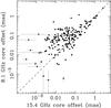 |
Fig. 1 Phase center offsets of the core components at 8.1 GHz versus that at 15.4 GHz taken from model fits. |
3. Method for measuring the core shift
Registration of two VLBI images taken at different frequencies provides a shift between the image phase centers, such that they are co-aligned to the same position on the sky. This image shift is not equal to the core shift we want to measure. In general, the presence of the jet structure we detect results in a non-zero offset of the core from the phase center. As the core components significantly dominate in total flux, the magnitude of the offsets is typically small, but at the same time not negligible. When a distant jet component is brighter than the core, the offset can be large, as in the case of the quasar 0923+392, where the offset is about 2.6 mas. Extreme cases are discussed in Petrov et al. (2011). Moreover, these offsets are different at different frequencies for a given source, and become statistically larger at lower frequencies due to spectral properties of the jets. Figure 1 shows the core offsets at 15.4 and 8.1 GHz, with the median values being 36 and 81 μas, respectively.
The core position departures from the phase center thus have to be taken into account to
derive the core shifts. Because the image shift IS is
independent of the core component position, it measures the vector sum of the absolute core
shift CS
(| CS| = Δrcore, ν1ν2)
and the difference in the coordinates (offset shift relative to the map center)
OS:  (1)from which the magnitude and direction of the
core shift vector can be readily calculated.
(1)from which the magnitude and direction of the
core shift vector can be readily calculated.
We used the fast normalized cross-correlation (NCC) algorithm by Lewis (1995) to register the images across the frequencies. The algorithm allows one to apply frequency domain methods to calculate the unnormalized cross correlation and then efficiently normalizes it by using precomputed integrals of the images over the search area. Thus, spatial domain computation of the cross correlation function is not needed and for large images the decrease in computing time is significant. The features that were matched between the images were selected from the optically thin part of the jet and assumed to have constant spectral index across them. The effect of possible spectral index gradients across the features is discussed in Sect. 5. In all cases, the image shifts IS, obtained with NCC, were verified by visually inspecting the corresponding spectral index images before and after the alignment, because the latter are extremely sensitive to the (in)accurate image alignment, as was shown by Kovalev et al. (2008). The spectral index images are presented and discussed by Hovatta et al. (2012). The image shifts between 15.4 GHz and other bands are found to be within a range of 0 and 1.11 mas, with a median value of 0.13 mas. The extreme value of 1.11 mas was detected in 3C 273 between 15.4 and 8.4 GHz, where the peak of brightness at those two frequencies corresponds to different features in the source structure. In some rare cases (e.g., 1928+738 at epoch 2006 Apr. 28 of and 2128−123 at epoch of 2006 Oct. 6), when an optically thin, bright, compact jet component dominates in flux density, the image shift was measured to be zero, as expected for achromatic jet components. The accuracy of the two-dimensional cross-correlation technique is discussed in Sect. 5.
The magnitude of the core offset difference vector OS between 15.4 GHz and other bands ranged between 0 and 1.09 mas, with a median value of 0.05 mas. The maximum value of 1.09 mas holds also for quasar 3C 273 due to the same reason.
Derived core shift vectors.
4. Core shift measurement results
Substituting the results of model fitting and two-dimensional cross correlation into Eq. (1), we calculated the magnitude Δrcore, ν1ν2 and direction θcs of the 15.4−8.1, 15.4−8.4, and 15.4−12.1 GHz core shift vectors for 160, 158, and 147 sources (Table 1), respectively. For the other 31, 33, and 44 sources we could not measure the respective 15.4−8.1, 15.4−8.4, and 15.4−12.1 core shifts, mostly due to the weakness of their jet emission (especially at 15.4 GHz). This made the cross-correlation technique inapplicable, since there was no sufficiently large optically thin emission structure for feature matching. We also excluded those sources, mostly nearby galaxies listed in Table 2, whose core region was complex (e.g., 3C 84, M 87; the core shift in M 87 was studied by Hada et al. 2011, using phase-referencing VLBA observations) or for which the identification of the core component was unclear (e.g., 0108+388, 1509+054). The maximum and median magnitude of the derived 15.4−8.1, 15.4−8.4, and 15.4−12.1 GHz core shift vectors in angular and linear scale are summarized in Table 3. As seen from Table 3, the median values of the 15.4−8.1 and 15.4−8.4 GHz core shifts are comparable, while the 15.4−12.1 GHz ones are statistically smaller, as expected. In angular scale, these values are of about 8% of the corresponding FWHM beam size at 8.1 GHz.
Sources excluded from the analysis due to unclear core position.
Core shift statistics.
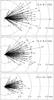 |
Fig. 2 Polar plots of the 15.4−8.1 (top), 15.4−8.4 (middle), and 15.4−12.1 GHz (bottom) core shift vectors. The polar axis is pointing to the right and co-aligns with the median jet direction of a source. Radial distance is given in mas. Dotted lines are drawn at intervals of 30°. |
In Fig. 2, we present plots of the derived core shifts in polar coordinates, where the head of each core shift vector represents the core position at lower frequency, while all core positions at higher frequency are placed at the origin. The polar axis corresponds to the median jet direction θjet calculated from position angles of the jet components with respect to the core component, using a corresponding model fit at 15.4 GHz. Thus the polar coordinates of the head of each vector represent the magnitude of the core shift vector, Δrcore,ν1ν2, and the angular deviation from the jet direction, θcs − θjet. The shift effect occurs predominantly along the jet direction. In more than 80% of cases, the core shift vectors deviate less than 45° from the median jet position angle. Statistically, the larger core shifts have better alignment with the jet direction because (i) they are less influenced by random errors and (ii) the core shift takes place along the jet in most cases. The weighted average of θcs − θjet is close to zero. Significant angular deviations of the core shift vectors from the median jet direction may take place in sources with substantial jet bending, either within an unresolved region near the VLBI core, or in the outer jet, thus affecting the median jet position angle. We have also analyzed distributions of the angular deviation between the core shift vectors and (i) inner jet direction determined as a position angle of the innermost jet component at 15.4 GHz and (ii) flux density-weighted average of the position angles of all Gaussian jet components at 15.4 GHz. In both these cases the scatter was larger, indicating that the median jet position angle is a better estimate for the direction of the outflow for the majority of sources.
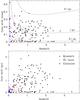 |
Fig. 3 Top: 15.4−8.1 GHz core shift in angular scale versus redshift. The dashed lines correspond to a fixed projected linear scale of 0.1, 1, and 3.1 pc. The latter curve envelopes all the measurements. Bottom: 15.4−8.1 GHz core shifts in projected linear scale versus redshift. Typical error values are discussed in Sect. 5. |
Our median 15.4−8.1 GHz core shift of 0.128 mas exceeds that of 0.080 mas reported by Sokolovsky et al. (2011), which was based on a smaller sample of 20 sources, for which the core shifts were derived using the self-referencing method. But if the 15.4−8.1 GHz core shifts for the 20-source sample are calculated from the fitted hyperbolas (Sokolovsky et al. 2011), which provide more accurate core shift values, the corresponding median yields 0.127 mas, which agrees well with the median of our sample.
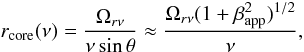
The sources with the largest angular shifts are all at z < 1, as shown in Fig. 3 (top), where we plot the 15.4−8.1 GHz core shift against redshift values. All measurements are confined under the aspect line corresponding to 3.1 pc, the maximum linear 15.4−8.1 GHz shift (see Table 3). In contrast, in linear projected scale (Fig. 3, bottom), low-redshift sources are characterized by small shifts due to quick falling of the scale factor, while more distant sources have larger shifts. We have found evidence that the angular core shift decreases with increasing redshift by binning the data into nine equally populated bins, though we cannot claim the dependence to be highly significant due to the large scatter in measured core shifts, which stems from different physical conditions and viewing angles in different sources at the same redshift. The plots for 15.4−8.4 and 15.4−12.1 GHz core shifts are qualitatively similar to Fig. 3.
Additionally, we tested whether the core shift measurements are affected by limited angular resolution blending following the approach used by Kovalev et al. (2008). If present, this effect would preferentially increase the magnitude of the core shift vectors when they are better aligned with the major axis of the interferometric restoring beam resulting in a U-shape dependence between Δrcore, ν1ν2 and |θcs − θbpa|, where θbpa is the position angle of the major axis of the beam, and −90 ≤ θbpa ≤ 90. We found no such trend in the 15.4−8.1 GHz measurements, confirming that the registered core shifts are not dominated by blending.
5. Accuracy of the method
5.1. Random errors
As seen from Eq. (1), the uncertainty of the core shift σν1ν2 is determined by errors of the core positions and image registration. However, individual a posteriori estimates of the image registration accuracy are problematic, since (1) in our case the values of the applied similarity criterion (NCC) are not normally distributed, making an estimation of random errors difficult, and since (2) systematic errors can only be addressed by simulations. Therefore, we used a statistical approach to assess the typical random core shift error in our sample. If we assume that (i) the core shift occurs along the jet and (ii) the errors are random in direction and comparable to each other, then the standard deviation of the transverse projections of the core shift vectors onto the jet direction yields the typical error. In Fig. 4, we plot the corresponding 15.4−8.1, 15.4−8.4, and 15.4−12.1 GHz distributions, from which we find σ15.4−8.1 GHz = 50 μas, σ15.4−8.4 GHz = 51 μas, and σ15.4−12.1 GHz = 35 μas. From these values, we determine that in 57%, 59%, and 58% of cases the respective core shifts are significantly (>2σ) different from zero, more than 90% of which in turn deviate less than 30° from the median jet direction. The derived error estimates are conservative, since in some cases the angular deviations of the core shift vector from the median jet direction can be real, for instance, in curved jets.
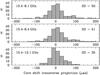 |
Fig. 4 Distributions of transverse projections of the 15.4−8.1, 15.4−8.4, and 15.4−12.1 GHz core shift vectors onto the jet direction. |
An alternative way to estimate a typical random error in core shift is based on the fact that 8.1 and 8.4 GHz bands are closely separated, but were processed independently. Therefore, the 15.4−8.1 and 15.4−8.4 GHz core shifts are expected to be virtually the same and the non-zero difference between them is due purely to errors. This approach was also used in Sokolovsky et al. (2011). Constructing a distribution of these differences and calculating its standard deviation, we found σ15.4−8.1 GHz ≈ σ15.4−8.4 GHz ≈ 55 μas, which is consistent with the error estimates obtained using the first method.
Since there is some freedom in selecting the jet feature to be matched in NCC, there is a possibility that user decisions affect the image registration results. We tested the robustness of the registration algorithm to “user bias” by having two different people separately perform the image alignment for one of the observing epochs. They both had similar instructions regarding the selection of the matched feature, i.e., (1) it should be optically thin, (2) and it should have as much structural variation as possible. The distribution of the differences in IS had a standard deviation of ≈ 50 μas for N = 24 pairs of images. This also closely matches the typical random error estimated above.
5.2. Systematic errors
So far we have discussed random errors, but the image registration method is also prone to systematic errors that may bias our core shift measurements. Namely, the assumption of a constant spectral index across the matched features does not necessarily hold in real jets. Indeed, it is known that spectral index gradients occur along the jet. The spectral index images between 8.1 and 15.4 GHz typically show gradients in the optically thin part of the jet from −0.3 mas-1 to +0.1 mas-1 with an average of ~− 0.1 mas-1 (Hovatta et al. 2012).
We tested the systematic effect that such gradients may have on image registration results by performing simulations. For the simulations we selected five sources with different jet morphologies: NGC 315 (straight, long and very smooth jet), 0716+714 (straight, short and smooth jet; Fig. 5, top), 3C 273 (long, wiggling jet with prominent knots; Fig. 6, top), BL Lac (wide, curved jet having one prominent knot downstream of the core), and 3C 454.3 (complex, curved jet with knots). For each source we created three sets of simulated images at six different frequencies exhibiting three different spectral index gradients along the jet: −0.1, −0.2, and −0.3 mas-1. The simulated images were based on a real 15.4 GHz image of a given source, to which a constant spectral index gradient along the jet was applied and new images at frequencies of 1.25, 1.50, 1.75, 2.00, 2.25, and 2.50 times the original frequency were calculated. Finally, random noise at the same level as in the original image was added to simulated images to ensure that background noise patterns between the images do not correlate. The original image and the simulated one were then registered using NCC. Note that this simulation setup provides a worst-case scenario in the sense that the gradient is assumed to be constant for the whole jet length, whereas in the real jets this is typically not the case.
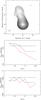 |
Fig. 5 Naturally weighted total intensity CLEAN image of 0716+714 at 15.4 GHz (top). The alignment error (in beam widths) along the jet as a function of frequency ratio (middle). The alignment error (in beam widths) perpendicular to the jet (bottom). The error is defined as rν1 − rν2 where rν1 is the position in the low-frequency image and rν2 is the corresponding position in the high-frequency image. The different spectral index gradients are shown in different colors: −0.1 mas-1 (black squares), −0.2 mas-1 (blue crosses), and −0.3 mas-1 (red circles). |
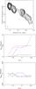 |
Fig. 6 Naturally weighted total intensity CLEAN image of 3C 273 at 15.4 GHz (top). The alignment error (in beam widths) along the jet as a function of frequency ratio (middle). The alignment error (in beam widths) perpendicular to the jet (bottom). The error is defined as rν1−rν2 where rν1 is the position in the low-frequency image and rν2 is the corresponding position in the high-frequency image. The different spectral index gradients are shown in different colors: −0.1 mas-1 (black squares), −0.2 mas-1 (blue crosses), and −0.3 mas-1 (red circles). |
The simulation results show that spectral index gradients along the jet can indeed affect the registration results and that the systematic error introduced this way depends on the jet morphology, the magnitude of the gradient, and the frequency ratio of the registered pair of images. In 3C 273 and BL Lac, which have significant structural detail in the optically thin part of the jet, the errors in the registered shift along the jet are less than 5% and less than 3% of the beam size, respectively, for all values of the gradient and for frequency ratios lower than 2. For 3C 273, a gradient of −0.1 mas-1 results in an error that is less than 1% of the beam size (Fig. 6, middle). The jet in 3C 454.3 also has significant structural detail, and the systematic errors for a gradient of −0.1 mas-1 stay below 4% of the beam size. However, for steeper gradients, the errors increase significantly, being less than ~10% of the beam size for frequency ratios below 2. The featureless jets of NGC 315 and 0716+714 are the most prone to systematic errors caused by spectral index gradients along the jet: even the flattest gradient results in errors in the range of 10−18% of the beam size. In 0716+714 the gradients of −0.2 and −0.3 mas-1 result in errors of 24% and 27% of the beam size, respectively, at a frequency ratio of 2 (Fig. 5, middle). In NGC 315 the steeper gradients cause a significant jump in the image shift that exceeds the beam size.
The above simulation demonstrates that the level of detail in the optically thin part of the jet is crucial for the reliability of the cross-correlation based image registration. If the jet has knots or bends, cross-correlation is rather robust against possible spectral index gradients. On the other hand, the method clearly does not work with smooth, straight jets that exhibit spectral index gradients. Also, the direction of the erroneous image shift due to spectral index gradient along these smooth, straight jets is such that it can mimic a true core shift. Therefore, we have repeated the core shift analysis in a “clean sample” from which such jets are removed. Statistics on the clean sample that comprises 94 sources, however, did not show lower median values for 15.4−8.1, 15.4−8.4, and 15.4−12,1 GHz core shift distributions. This indicates that the effect of a possible overestimation of image shifts (and consequently core shifts) owing to a spectral index gradient along the jet is weak.
We also estimated positional errors (from the image plane) of the core components using the relation suggested by Fomalont (1999): (W·RMS)/(2P), where W and P are the convolved size and peak intensity of the component, RMS is the post-fit rms error associated with the pixels in a nine-beam area region under the component in the residual image. Because the cores are bright and compact, their signal-to-noise ratio S/N = P/RMS values are high, with a median value of a few hundred, making the corresponding positional errors small, with a median value of about 1 μas. This implies that the core shift error is typically dominated by the uncertainty of the image alignment for a sample of core-dominated AGN jets.
The typical accuracy level of about 50 μas achieved in our core shift measurements is comparable to that from the self-referencing approach (Sokolovsky et al. 2011), where the errors are dominated by position uncertainties of a referencing jet component, which is usually larger in size and weaker in flux density with respect to the core. Phase-referencing observations may provide slightly better accuracy, down to 30 μas, for the 15.4−8.4 GHz core shift, as reported by Hada et al. (2011), but cannot be used for a large number of sources as discussed in Sect. 1. Another complication of the phase-referencing method comes from the fact that the calibrator has its own core shift.
5.3. Stationary jet feature problem
Jets can exhibit standing features, like re-collimation shocks, in or close to their core region and these features could in principle introduce a level of artificial core shift owing to the degradation of the angular resolution with wavelength. To study how strong an effect these standing features could have, we used the AIPS task UVMOD to create simulated VLBA data sets at 8.1, 8.4, 15.3, 23.8, and 43.2 GHz. We used a real multi-wavelength VLBA observation to provide the (u,v) plane sampling and noise properties at every frequency, and as an input model for UVMOD we used three Gaussian components representing the core, a standing feature, and a jet feature. A set of simulated (u,v) data was generated with different flux ratios between the core and the standing feature (ranging from 10% to 50%) and with different distances between the two (0.15 mas and 0.3 mas). As a result, we had a simulated multi-wavelength VLBA data set in which all wavelengths had exactly the same sky brightness distribution, but different (u,v) sampling and noise. Any apparent core-shift in this data set would be purely caused by the (u,v) coverage differences at different frequencies. Analyzing the simulated data sets, we found that a close (within 0.3 mas from the 43 GHz core) standing jet feature can contribute to the expected core shift effect between 43 GHz and 8 GHz owing to frequency-dependent blending on the level of ~10% of the expected core shift if the flux density ratio of the stationary feature and the core Sst/Sc ~ 10%, and reaching up to ~30% of the expected core shift if Sst/Sc ~ 50%. Between the frequencies used in this study, i.e., 15 and 8 GHz, the core shift is affected by the frequency-dependent blending by ≲ 20 μas, which is less than the estimated accuracy of our measurements. We note that these simulations describe a very simple situation and a more detailed study of the effect of stationary features to the measured core shift using real data is warranted. However, this is beyond the scope of the current work.
6. Jet physics with core shifts
To increase the robustness of our subsequent calculations, from now on we use a vector average for each pair of the 15.4−8.1 and 15.4−8.4 GHz core shifts. Moreover, if the core shift magnitude is smaller than 1 sigma level, we set Δrcore 15−8 = σ15−8 = 51 μas to be used as the upper limit, since eliminating the small core shifts would introduce a bias. We excluded only the core shift vectors with |θcs − θjet| > 90°, which are likely to be dominated by errors. In total, we have core shifts between 15 and 8 GHz for 136 sources, 108 of which have both redshift (Fig. 7, left) and apparent jet speed measurements. If a source had a second epoch, we selected the one at which the dynamic range of the 15 GHz image was higher.
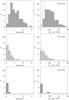 |
Fig. 7 Distribution of redshift (left) and core shift measure Ωrν (right) for 136 sources with the core shift derived between 15 and 8 GHz. Gray filled bins represent 98 quasars (top), dashed bins represent 28 BL Lacs (middle), and cross-hatched bins represent 10 galaxies (bottom). Empty bins show upper limits. |
As shown by Lobanov (1998), core shift measurements
can be used for deriving a variety of physical conditions in the compact jets. In
particular, assuming equipartition between the particle and magnetic field energy density
(kr = 1) and a jet spectral index
αjet = −0.5
(S ∝ ν+α), the magnetic
field in Gauss at 1 pc of actual distance from the jet vertex can be calculated through the
following proportionality (Hirotani 2005; O’Sullivan & Gabuzda 2009) 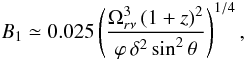 (2)where ϕ is the half jet
opening angle, θ is the viewing angle, δ is the Doppler
factor, and Ωrν is the core shift measure defined in Lobanov (1998) as
(2)where ϕ is the half jet
opening angle, θ is the viewing angle, δ is the Doppler
factor, and Ωrν is the core shift measure defined in Lobanov (1998) as
 (3)where
Δrcore, ν1ν2
is the core shift in milliarcseconds, and DL is
the luminosity distance in parsecs. The calculated values of Ωrν
in pc GHz form a distribution ranging from 0.8 to 54.1 and peaking near the median of 13.6
(Fig. 7, right). The distributions of
Ωrν for quasars and BL Lacs are significantly different
(p < 10-4) as indicated by Gehan’s generalized Wilcoxon
test from the ASURV survival analysis package (Lavalley
et al. 1992), with medians of 18.6 and 7.1 pc GHz, respectively.
(3)where
Δrcore, ν1ν2
is the core shift in milliarcseconds, and DL is
the luminosity distance in parsecs. The calculated values of Ωrν
in pc GHz form a distribution ranging from 0.8 to 54.1 and peaking near the median of 13.6
(Fig. 7, right). The distributions of
Ωrν for quasars and BL Lacs are significantly different
(p < 10-4) as indicated by Gehan’s generalized Wilcoxon
test from the ASURV survival analysis package (Lavalley
et al. 1992), with medians of 18.6 and 7.1 pc GHz, respectively.
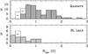 |
Fig. 8 Distribution of magnetic field at a distance of 1 pc from the black hole for 84 quasars (top), 18 BL Lacs (bottom). Empty bins represent upper limits. |
The combination of ϕ, δ, and θ in
Eq. (2) is typically known for only a small
fraction of sources, limiting the applicability of the formula. Therefore, the number of
sources in our subsample with known apparent jet speed βapp
(Lister et al. 2009) is larger by a factor of
>2 than the number of sources with known variability Doppler factor (Hovatta et al. 2009), intrinsic opening angle and viewing
angle (e.g. Pushkarev et al. 2009; Savolainen et al. 2010). The denominator in (2) can be expressed through
βapp only by substituting
δ = Γ-1(1 − βcosθ)-1
and  , and also taking into account that
2ϕ ≃ 0.26 Γ-1 (Pushkarev
et al. 2009) and
βapp = βsinθ (1 − βcosθ)-1.
With these substitutions we are assuming the the jet is viewed at the critical angle
θ ≃ Γ-1 that maximizes βapp. We
therefore obtain
, and also taking into account that
2ϕ ≃ 0.26 Γ-1 (Pushkarev
et al. 2009) and
βapp = βsinθ (1 − βcosθ)-1.
With these substitutions we are assuming the the jet is viewed at the critical angle
θ ≃ Γ-1 that maximizes βapp. We
therefore obtain  (4)where for βapp we
use the fastest non-accelerating, radial apparent speed measured in the source (Lister et al. 2009).
(4)where for βapp we
use the fastest non-accelerating, radial apparent speed measured in the source (Lister et al. 2009).
First, we tested the consistency of B1 values calculated from
Eqs. (2) and (4) for sources with previously measured δ
and βapp values. For 40 sources out of 43 in common,
comprising 35 quasars and 8 BL Lacs, the results agree within the errors, with a median
value of their ratio of 0.99. For three sources (0420−014, 0804+499, and 1413+135),
Eq. (2) gives several times higher values,
most probably due to underestimated apparent speeds, to which (2) is more sensitive than (4), because the viewing angle ![Mathematical equation: \hbox{$\theta=\arctan[2\beta_\mathrm{app}(\beta_\mathrm{app}^2+\delta^2-1)^{-1}]$}](/articles/aa/full_html/2012/09/aa19173-12/aa19173-12-eq91.png) and the opening
angle ϕ = ϕobssinθ. Indeed,
these sources have low apparent speeds but high Doppler factors, leading to low viewing
angle estimates of
and the opening
angle ϕ = ϕobssinθ. Indeed,
these sources have low apparent speeds but high Doppler factors, leading to low viewing
angle estimates of  ,
,  ,
,  (Savolainen
et al. 2010), respectively, and in turn to overestimated magnetic field strengths.
The uncertainties in B1 from Eq. (4) were calculated taking into account the errors in the core shifts,
apparent speeds, and also from the assumption θ ≃ Γ-1, which is
known to introduce an additional source of errors, as discussed by Lister (1999). Since the aforementioned assumption is less correct for
sources with low Lorentz factors, we excluded galaxies from the subsequent analysis.
(Savolainen
et al. 2010), respectively, and in turn to overestimated magnetic field strengths.
The uncertainties in B1 from Eq. (4) were calculated taking into account the errors in the core shifts,
apparent speeds, and also from the assumption θ ≃ Γ-1, which is
known to introduce an additional source of errors, as discussed by Lister (1999). Since the aforementioned assumption is less correct for
sources with low Lorentz factors, we excluded galaxies from the subsequent analysis.
Jet parameters derived for the sources with significant core shifts between 8 and 15 GHz.
The distributions of B1 values derived from Eq. (4) for 84 quasars and 18 BL Lacs shown in
Fig. 8 have medians
of  and
and  G, respectively, where the errors derived
from a bootstrapping method indicate 95% confidence intervals. Gehan’s generalized Wilcoxon
test from the ASURV survival analysis package indicates that the distributions of
B1 for quasars and BL Lacs are different at 99.6% confidence
level. The difference is driven mainly by statistically higher redshifts for the quasars,
and, though to a lesser degree, also by higher βapp (Fig. 9). The B1 values would be
comparable for these classes of objects, if the ratio of the median core shifts for BL Lacs
to that of quasars was about 2.7, but that is not the case. Systematically stronger magnetic
fields in quasars can be a result of more massive black holes hosted by them and/or higher
accretion rate in these objects, because larger black holes can accrete more matter,
effectively powering the jets and accelerating particles to higher speeds. This scenario is
also supported by an indication for quasars to have on average narrower intrinsic opening
angles than those of BL Lacs, as reported by Pushkarev
et al. (2009). At the same time, Woo & Urry
(2002) argued that BL Lacs host black holes of comparable mass to quasars, though
the estimates of black hole masses for quasars and BL Lacertae objects have been generated
by different methods, and this may introduce a bias while comparing the mass assessments.
G, respectively, where the errors derived
from a bootstrapping method indicate 95% confidence intervals. Gehan’s generalized Wilcoxon
test from the ASURV survival analysis package indicates that the distributions of
B1 for quasars and BL Lacs are different at 99.6% confidence
level. The difference is driven mainly by statistically higher redshifts for the quasars,
and, though to a lesser degree, also by higher βapp (Fig. 9). The B1 values would be
comparable for these classes of objects, if the ratio of the median core shifts for BL Lacs
to that of quasars was about 2.7, but that is not the case. Systematically stronger magnetic
fields in quasars can be a result of more massive black holes hosted by them and/or higher
accretion rate in these objects, because larger black holes can accrete more matter,
effectively powering the jets and accelerating particles to higher speeds. This scenario is
also supported by an indication for quasars to have on average narrower intrinsic opening
angles than those of BL Lacs, as reported by Pushkarev
et al. (2009). At the same time, Woo & Urry
(2002) argued that BL Lacs host black holes of comparable mass to quasars, though
the estimates of black hole masses for quasars and BL Lacertae objects have been generated
by different methods, and this may introduce a bias while comparing the mass assessments.
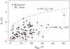 |
Fig. 9 Magnetic field at a distance of 1 pc from the central black hole versus fastest non-accelerating, radial apparent speed. The measurements are enveloped under the dashed aspect line. The middle dotted line shows the dependence based on the medians for redshift and core shift measure Ωrν. |
The absolute distance in parsecs of the apparent VLBI core measured from the jet vertex is
given by (Lobanov 1998)
 (5)where ν is the observed
frequency in GHz. Then the corresponding magnetic field strength
is
(5)where ν is the observed
frequency in GHz. Then the corresponding magnetic field strength
is  . In Fig. 10, we plot the derived rcore
and Bcore for the 15 GHz cores. Note that the core magnetic
fields show a reverse tendency compared to the B1 values, with a
median of 0.10 G for BL Lacs and 0.07 G for quasars, because their apparent cores are at
different separations from the true jet base, with medians of 4.0, and 13.2 pc,
respectively.
. In Fig. 10, we plot the derived rcore
and Bcore for the 15 GHz cores. Note that the core magnetic
fields show a reverse tendency compared to the B1 values, with a
median of 0.10 G for BL Lacs and 0.07 G for quasars, because their apparent cores are at
different separations from the true jet base, with medians of 4.0, and 13.2 pc,
respectively.
On the projected plane (i.e., a VLBI map), the median separation of the 15 GHz core from the central black hole is about 1 pc, corresponding to about 0.14 mas for a source at z ≃ 1. We summarize the derived physical quantities, such as Ωrν, B1, Bcore, and rcore in Table 4.
 |
Fig. 10 Magnetic field in the 15 GHz core versus its deprojected separation from the true jet base. The dashed line is the linear least-squares fit for quasar measurements. |
The mass of a central black hole can be related to B1, such
that
Mbh ≈ 2.7 × 10⁹B1 M⊙
(Lobanov 1998). Its typical value is
~109 M⊙ for quasars and BL Lacs.
B1 can also be used to estimate the magnetic field
BBH near the central black hole, assuming a
B ∝ R-1 dependence, where R
is the half-width of the jet. Thus, we have
BBH = B1R1/RBH,
where R1 and RBH are the the
half-widths of the jet at 1 pc from the jet vertex and near the black hole, respectively. To
derive R1, we assume that the jet is conical at distances larger
than 1 pc. Then, we
have R1 = Rcore − (rcore − 1)tanϕ,
where Rcore is the half-width of the 15 GHz core,
rcore is the 15 GHz core separation from the jet vertex (both
measured in pc), and ϕ is the intrinsic half jet opening angle. Because the
black hole masses for BL Lacs are poorly known due to their weak emission lines, we restrict
our analysis to quasars only. We derived the following median values:
 (Pushkarev
et al. 2009), rcore = 13.2 pc,
Rcore = 0.35 pc. Then R1 ≈ 0.2 pc
and BBH ≈ 2 × 10³ G, assuming the jet width near the
~109 M⊙ black hole to be on the order of
its gravitational radius. The derived assessment of the magnetic field near the black hole
is consistent with the theoretical value calculated from a model of a thin, magnetically
driven accretion disk (Field & Rogers 1993).
(Pushkarev
et al. 2009), rcore = 13.2 pc,
Rcore = 0.35 pc. Then R1 ≈ 0.2 pc
and BBH ≈ 2 × 10³ G, assuming the jet width near the
~109 M⊙ black hole to be on the order of
its gravitational radius. The derived assessment of the magnetic field near the black hole
is consistent with the theoretical value calculated from a model of a thin, magnetically
driven accretion disk (Field & Rogers 1993).
7. Summary
We have implemented a method for measuring the frequency-dependent shift in absolute position of the parsec-scale core and applied it to multi-frequency (8.1, 8.4, 12.1, and 15.4 GHz) VLBA observations of 191 sources performed during 2006 within the MOJAVE program. The method is based on results from (i) image registration achieved by a two-dimensional cross-correlation technique and (ii) structure model fitting. It has proved to be very effective and provided the core shifts in 163 sources (85%), with a median of 128 μas between 15 and 8 GHz, and 88 μas between 15 and 12 GHz. Despite the moderate separation of the observing frequencies, the derived core shifts are significant (>2σ) in about 55% of cases, given an estimated typical uncertainty of 50 μas between 15 and 8 GHz, and 35 μas between 15 and 12 GHz. The errors are dominated by uncertainties from the two-dimensional cross-correlation procedure, because the relative positional uncertainties of the compact bright cores are at a level of a few microarcseconds. The significant core shift vectors are found to be preferentially aligned with the median jet direction, departing from it by less than 30° in more than 90% of cases.
We used the measured core shifts for constraining magnetic field strengths and core sizes for 89 sources. The magnetic field at a distance of 1 pc from the jet injection point is found to be ~0.9 G for quasars and ~0.4 G for BL Lacs. Extrapolating all the way back by assuming a B ∝ R-1 dependence, the magnetic field in the close vicinity of the black hole is about 2 × 10³ G. The core sizes, i.e., the distances from the true jet base to its apparent origin at 15.4 GHz are statistically larger in quasars than in BL Lacs, with a median of 13.2 and 4.0 pc, respectively. At these distances, the magnetic field has a median of 0.07 G for quasars and 0.1 G for BL Lacertae objects.
Future multi-epoch and multi-frequency VLBI observations (including phase-referencing) of a pre-selected sample of sources with prominent core shifts are needed to address the question of the core shift variability, which can be used not only for astrophysical studies but also for astrometric applications. Ideally, these observations should be performed during and after strong nuclear flares that can be detected in advance in higher energy domains, e.g., optical or gamma-ray, and cover a wide range of observing frequencies, extending down to 5 or 2 GHz, where synchrotron self-absorption is essential.
Online material
Derived core shift vectors.
Derived jet parameters.
Acknowledgments
We would like to thank K. I. Kellermann, E. Ros, D. C. Homan and the rest of the MOJAVE team for the productive discussions. We thank the anonymous referee for useful comments, which helped to improve the manuscript. This research has made use of data from the MOJAVE database that is maintained by the MOJAVE team (Lister et al. 2009). The MOJAVE project is supported under National Science Foundation grant AST-0807860 and NASA Fermi grant NNX08AV67G. T.H. was supported in part by the Jenny and Antti Wihuri foundation. Y.Y.K. is partly supported by the Russian Foundation for Basic Research (project 11-02-00368), Dynasty Foundation, and the basic research program “Active processes in galactic and extragalactic objects” of the Physical Sciences Division of the Russian Academy of Sciences. Part of this work was supported by the COST Action MP0905 “Black Holes in a Violent Universe”. The VLBA is a facility of the National Science Foundation operated by the National Radio Astronomy Observatory under cooperative agreement with Associated Universities, Inc.
References
- Bietenholz, M. F., Bartel, N., & Rupen, M. P. 2004, ApJ, 615, 173 [NASA ADS] [CrossRef] [Google Scholar]
- Blandford, R. D., & Königl, A. 1979, ApJ, 232, 34 [Google Scholar]
- Croke, S. M., & Gabuzda, D. C. 2008, MNRAS, 386, 619 [CrossRef] [Google Scholar]
- Field, G. B., & Rogers, R. D. 1993, ApJ, 403, 94 [NASA ADS] [CrossRef] [Google Scholar]
- Fomalont, E. B. 1999, in Synthesis Imaging in Radio Astronomy II, eds. G. B. Taylor, C. L. Carilli, & R. A. Perley, ASP Conf. Ser., 180, 301 [Google Scholar]
- Fromm, C. M., Ros, E., Savolainen, T., et al. 2010 [arXiv:1011.4825] [Google Scholar]
- Greisen, E. W. 2003, in Information Handling in Astronomy – Historical Vistas, ed. A. Heck (Dordrecht: Kluwer), Astrophys. Space Sci. Libr., 285, 109 [NASA ADS] [Google Scholar]
- Guirado, J. C., Marcaide, J. M., Alberdi, A., et al. 1995, AJ, 110, 2586 [NASA ADS] [CrossRef] [Google Scholar]
- Hada, K., Doi, A., Kino, M., et al. 2011, Nature, 477, 185 [NASA ADS] [CrossRef] [Google Scholar]
- Hirotani, K. 2005, ApJ, 619, 73 [Google Scholar]
- Högbom, J. A. 1974, A&AS, 15, 417 [Google Scholar]
- Hovatta, T., Valtaoja, E., Tornikoski, M., & Lähteenmäki, A. 2009, A&A, 498, 723 [NASA ADS] [CrossRef] [EDP Sciences] [Google Scholar]
- Hovatta, T., Lister, M. L., Aller, M. F., et al. 2012, AJ, 144, 105 [Google Scholar]
- Hujeirat, A., Livio, M., Camenzind, M., & Burkert, A. 2003, A&A, 408, 415 [NASA ADS] [CrossRef] [EDP Sciences] [Google Scholar]
- Jennison, R. C. 1958, MNRAS, 118, 276 [Google Scholar]
- Junor, W., Biretta, J. A., & Livio, M. 1999, Nature, 401, 891 [NASA ADS] [CrossRef] [Google Scholar]
- Kadler, M., Ros, E., Lobanov, A. P., Falcke, H., & Zensus, J. A. 2004, A&A, 426, 481 [NASA ADS] [CrossRef] [EDP Sciences] [Google Scholar]
- Kellermann, K. I., Kovalev, Y. Y., Lister, M. L., et al. 2007, Ap&SS, 311, 231 [NASA ADS] [CrossRef] [Google Scholar]
- Koide, S., Shibata, K., Kudoh, T., & Meier, D. L. 2002, Science, 295, 1688 [NASA ADS] [CrossRef] [Google Scholar]
- Komatsu, E., Dunkley, J., Nolta, M. R., et al. 2009, ApJS, 180, 330 [NASA ADS] [CrossRef] [Google Scholar]
- Komissarov, S. S. 2005, MNRAS, 359, 801 [NASA ADS] [CrossRef] [Google Scholar]
- Königl, A. 1981, ApJ, 243, 700 [Google Scholar]
- Kovalev, Y. Y., Lobanov, A. P., Pushkarev, A. B., & Zensus, J. A. 2008, A&A, 483, 759 [NASA ADS] [CrossRef] [EDP Sciences] [Google Scholar]
- Kudryavtseva, N. A., Gabuzda, D. C., Aller, M. F., & Aller, H. D. 2011, MNRAS, 415, 1631 [NASA ADS] [CrossRef] [Google Scholar]
- Lara, L., Alberdi, A., Marcaide, J. M., & Muxlow, T. W. B. 1994, A&A, 285, 393 [NASA ADS] [Google Scholar]
- Lavalley, M., Isobe, T., & Feigelson, E. 1992, in Astronomical Data Analysis Software and Systems I, eds. D. M. Worrall, C. Biemesderfer, & J. Barnes, ASP Conf. Ser., 25, 245 [Google Scholar]
- Lewis, J. P. 1995, Vision Interface, 120 [Google Scholar]
- Lindegren, L., & Perryman, M. A. C. 1996, A&AS, 116, 579 [NASA ADS] [CrossRef] [EDP Sciences] [Google Scholar]
- Lister, M. L. 1999, Ph.D. Thesis, Boston University [Google Scholar]
- Lister, M. L., Aller, H. D., Aller, M. F., et al. 2009, AJ, 137, 3718 [Google Scholar]
- Lobanov, A. P. 1998, A&A, 330, 79 [NASA ADS] [Google Scholar]
- Lobanov, A. P., & Zensus, J. A. 2007, Exploring the Cosmic Frontier, eds. A. P. Lobanov, J. A. Zensus, C. Cesarsky, & P. J. Diamond (Springer-Verlag), 147 [Google Scholar]
- Marcaide, J. M., & Shapiro, I. I. 1984, ApJ, 276, 56 [Google Scholar]
- O’Sullivan, S. P., & Gabuzda, D. C. 2009, MNRAS, 400, 26 [Google Scholar]
- Petrov, L., Kovalev, Y. Y., Fomalont, E. B., & Gordon, D. 2011, AJ, 142, 35 [NASA ADS] [CrossRef] [Google Scholar]
- Pushkarev, A. B., Kovalev, Y. Y., Lister, M. L., & Savolainen, T. 2009, A&A, 507, L33 [NASA ADS] [CrossRef] [EDP Sciences] [Google Scholar]
- Ros, E., & Lobanov, A. P. 2001, in 15th Workshop Meeting on European VLBI for Geodesy and Astrometry, eds. D. Behrend, & A. Rius, 208 [Google Scholar]
- Savolainen, T., Homan, D. C., Hovatta, T., et al. 2010, A&A, 512, A24 [NASA ADS] [CrossRef] [EDP Sciences] [Google Scholar]
- Shepherd, M. C. 1997, in Astronomical Data Analysis Software and Systems VI, eds. G. Hunt, & H. E. Payne (San Francisco: ASP), ASP Conf. Ser., 125, 77 [Google Scholar]
- Sokolovsky, K. V., Kovalev, Y. Y., Pushkarev, A. B., & Lobanov, A. P. 2011, A&A, 532, A38 [CrossRef] [EDP Sciences] [Google Scholar]
- Twiss, R. Q., Carter, A. W. L., & Little, A. G. 1960, The Observatory, 80, 153 [NASA ADS] [Google Scholar]
- Vlahakis, N., & Königl, A. 2004, ApJ, 605, 656 [Google Scholar]
- Walker, R. C., Dhawan, V., Romney, J. D., Kellermann, K. I., & Vermeulen, R. C. 2000, ApJ, 530, 233 [Google Scholar]
- Woo, J.-H., & Urry, C. M. 2002, ApJ, 579, 530 [NASA ADS] [CrossRef] [Google Scholar]
All Tables
Jet parameters derived for the sources with significant core shifts between 8 and 15 GHz.
All Figures
|
Fig. 1 Phase center offsets of the core components at 8.1 GHz versus that at 15.4 GHz taken from model fits. |
| In the text | |
|
Fig. 2 Polar plots of the 15.4−8.1 (top), 15.4−8.4 (middle), and 15.4−12.1 GHz (bottom) core shift vectors. The polar axis is pointing to the right and co-aligns with the median jet direction of a source. Radial distance is given in mas. Dotted lines are drawn at intervals of 30°. |
| In the text | |
|
Fig. 3 Top: 15.4−8.1 GHz core shift in angular scale versus redshift. The dashed lines correspond to a fixed projected linear scale of 0.1, 1, and 3.1 pc. The latter curve envelopes all the measurements. Bottom: 15.4−8.1 GHz core shifts in projected linear scale versus redshift. Typical error values are discussed in Sect. 5. |
| In the text | |
|
Fig. 4 Distributions of transverse projections of the 15.4−8.1, 15.4−8.4, and 15.4−12.1 GHz core shift vectors onto the jet direction. |
| In the text | |
|
Fig. 5 Naturally weighted total intensity CLEAN image of 0716+714 at 15.4 GHz (top). The alignment error (in beam widths) along the jet as a function of frequency ratio (middle). The alignment error (in beam widths) perpendicular to the jet (bottom). The error is defined as rν1 − rν2 where rν1 is the position in the low-frequency image and rν2 is the corresponding position in the high-frequency image. The different spectral index gradients are shown in different colors: −0.1 mas-1 (black squares), −0.2 mas-1 (blue crosses), and −0.3 mas-1 (red circles). |
| In the text | |
|
Fig. 6 Naturally weighted total intensity CLEAN image of 3C 273 at 15.4 GHz (top). The alignment error (in beam widths) along the jet as a function of frequency ratio (middle). The alignment error (in beam widths) perpendicular to the jet (bottom). The error is defined as rν1−rν2 where rν1 is the position in the low-frequency image and rν2 is the corresponding position in the high-frequency image. The different spectral index gradients are shown in different colors: −0.1 mas-1 (black squares), −0.2 mas-1 (blue crosses), and −0.3 mas-1 (red circles). |
| In the text | |
|
Fig. 7 Distribution of redshift (left) and core shift measure Ωrν (right) for 136 sources with the core shift derived between 15 and 8 GHz. Gray filled bins represent 98 quasars (top), dashed bins represent 28 BL Lacs (middle), and cross-hatched bins represent 10 galaxies (bottom). Empty bins show upper limits. |
| In the text | |
|
Fig. 8 Distribution of magnetic field at a distance of 1 pc from the black hole for 84 quasars (top), 18 BL Lacs (bottom). Empty bins represent upper limits. |
| In the text | |
|
Fig. 9 Magnetic field at a distance of 1 pc from the central black hole versus fastest non-accelerating, radial apparent speed. The measurements are enveloped under the dashed aspect line. The middle dotted line shows the dependence based on the medians for redshift and core shift measure Ωrν. |
| In the text | |
|
Fig. 10 Magnetic field in the 15 GHz core versus its deprojected separation from the true jet base. The dashed line is the linear least-squares fit for quasar measurements. |
| In the text | |
Current usage metrics show cumulative count of Article Views (full-text article views including HTML views, PDF and ePub downloads, according to the available data) and Abstracts Views on Vision4Press platform.
Data correspond to usage on the plateform after 2015. The current usage metrics is available 48-96 hours after online publication and is updated daily on week days.
Initial download of the metrics may take a while.