| Issue |
A&A
Volume 544, August 2012
|
|
|---|---|---|
| Article Number | A89 | |
| Number of page(s) | 22 | |
| Section | Extragalactic astronomy | |
| DOI | https://doi.org/10.1051/0004-6361/201218852 | |
| Published online | 02 August 2012 | |
The parsec-scale jet of PKS 1749+096⋆
1 Key Laboratory for Research in Galaxies and Cosmology, Shanghai Astronomical Observatory, Chinese Academy of Sciences, 80 Nandan Rd, 200030 Shanghai, PR China
e-mail: This email address is being protected from spambots. You need JavaScript enabled to view it.
2 Graduate School of the Chinese Academy of Sciences, 100039 Beijing, PR China
3 Max-Planck-Institut für Radioastronomie, Auf dem Hügel 69, 53121 Bonn, Germany
4 Massachusetts Institute of Technology, Haystack Observatory, Route 40, Westford, MA 01886, USA
5 Key Laboratory of Radio Astronomy, Chinese Academy of Sciences, PR China
6 National Astronomical Observatory of Japan, 2-2-1 Osawa, Mitaka, 181-8588 Tokyo, Japan
7 Korean VLBI Network, Korea Astronomy and Space Science Institute, PO Box 88, Yonsei University, Seongsanro 262, Seodaemun, Seoul 120-749, Republic of Korea
Received: 20 January 2012
Accepted: 6 April 2012
Abstract
Context.PKS 1749+096 is a BL Lac object showing weak extended jet emission to the northeast of the compact VLBI core on parsec scales.
Aims. We aim at better understanding the jet kinematics and variability of this source and finding clues that may applicable to other BL Lac objects.
Methods. The jet was studied with multi-epoch multi-frequency high-resolution VLBI observations.
Results. The jet is characterized by a one-sided curved morphology at all epochs and all frequencies. The VLBI core, located at the southern end of the jet, was identified based on its spectral properties. The equipartition magnetic field of the core was investigated, through which we derived a Doppler factor of 5, largely consistent with that derived from kinematics (component C5). The study of the detailed jet kinematics at 22 and 15 GHz, spanning a period of more than 10 years, indicates the possible existence of a bimodal distribution of the jet apparent speed. Ballistic and non-ballistic components are found to coexist in the jet. Superluminal motions in the range of 5–21 c were measured in 11 distinct components. We estimated the physical jet parameters with the minimum Lorentz factor of 10.2 and Doppler factors in the range of 10.2–20.4 (component C5). The coincidence in time of the component’s ejection and flares supports the idea that, at least in PKS 1749+096, ejection of new jet components is connected with major outbursts in flux density. For the best-traced component (C5) we found that the flux density decays rapidly as it travels downstream the jet, accompanied by a steepening of its spectra, which argues in favor of a contribution of inverse Compton cooling. These properties make PKS 1749+096 a suitable target for an intensive monitoring to decipher the variability phenomenon of BL Lac objects.
Key words: quasars: individual: PKS 1749+096 / galaxies: jets / radio continuum: galaxies
Figure A.1 and Tables A.1, A.2 are available in electronic form at http://www.aanda.org
© ESO, 2012
1. Introduction
PKS 1749 + 096 (also known as OT 081 and 4C +09.57) is an ultra-luminous BL Lac object with an optical polarization of up to 32% (Fan & Lin 1999). Dallacasa et al. (2000) classified this source as a high-frequency peaker (HFP), while Torniainen et al. (2005) suggested that it is a flat-spectrum source with an inverted spectrum during flares. Strong variability is often seen from the radio to X-ray regime. The variability at high radio frequencies is outstanding: the quiescent flux density is less than 1 Jy and during the outbursts the source reached up to more than 10 Jy with the fractional variability index, defined as VarΔS = (Smax − Smin)/Smin, about 13 and 18 at 37 and 90 GHz, respectively (Torniainen et al. 2005). In gamma-ray band, it was recently detected with Fermi (Abdo et al. 2009) though no counterpart was found by EGRET according to Mattox et al. (2001).
This compact BL Lac object was unresolved on arc-second scales by VLA observations (Rector & Stocke 2003). On mas scales, it was dominated by the compact, strong core, which contains over 90% of its total flux (Homan et al. 2001, and references therein), and showed a curved structure with faint jet features extending to northeast (e.g., Gabuzda et al. 1999; Lister & Homan 2005). Superluminal motion of jet features in PKS 1749+096 has been reported with apparent speeds in the range of ~ 1–14 c(Iguchi et al. 2000; Homan et al. 2001; Kellermann et al. 2004; Lister et al. 2009a). PKS 1749+096 is also among the most compact sources investigated with 215 GHz VLBI (Krichbaum et al. 1997). Therefore it is suitable for VLBI studies at short millimeter wavelengths.
In this paper, we present results from high-resolution VLBI studies of PKS 1749+096. In Sect. 2, we describe the observations and data analysis. In Sect. 3, we present results followed by discussion in Sect. 4. Finally, a brief summary is given in Sect. 5. At a redshift of 0.32 (Stickel et al. 1988), the luminosity distance to PKS 1749+096 is DL = 1674 Mpc and 1 mas of angular separation corresponds to 4.64 pc, a proper motion of 0.1 mas yr-1 corresponds to a speed of βapp = 2.0 c (adopting H0 = 71 km s-1 Mpc-1, ΩM = 0.27, ΩΛ = 0.73). Throughout this paper, the spectral index α is defined by Sν ∝ να.
2. Observations and data analysis
VLBI observations of PKS 1749+096 at 22 GHz were made for projects to investigate OVV 1633+382 after a major flare (code: BK090, BK092, and BK107), where PKS 1749+096 was observed as a fringe finder. These observations were performed with VLBA (BK090 and BK092) and VLBA plus the Effelsberg telescope (BK107) roughly every 2–3 months from December 2001 to February 2005 (14 epochs in total). Data were recorded with four IFs in left and right circular polarization with an IF bandwidth of 8 MHz and two-bit sampling, giving a data rate of 256 Mbps (except in 2001.937 with a data rate of 128 Mbps, two IFs in each polarization). The typical on-source integration time was about 20 min.
To study the jet kinematics for PKS 1749+096 in more detail, 42 epoch data at 15 GHz from the “2 cm Survey” and the follow up MOJAVE1 program between 1995 and 2005, spanning 11 years, were analyzed. Part of these data have been used to investigate the statistical properties of a sample of active galaxies (Homan et al. 2001; Lister et al. 2009b). Moreover, Iguchi et al. (2000) made observations of this source at four frequencies including 15 GHz with the VLBA in 1998, which we re-calibrated and re-mapped. In addition to these 15 GHz data, two simultaneous multi-frequency (8, 15, 22, and 43 GHz) data sets for PKS 1749+096 from the VLBA archive on May 07, 1999 (code: BI012) and on September 13, 2001 (code: BI018) were analyzed. These observations were made in frequency-switch mode and the data were recorded in VLBA format in left circular polarization (LCP) (1999) and in dual circular polarization (2001) with four IFs of 8 MHz each. Two-bit sampling was used in the recording. In each frequency, the total integration time was ~100 (1999) and ~40 (2001) min.
The archival 15 GHz data from the 2 cm/MOJAVE observing program were provided as fringe-fitted and calibrated uv FITS files, which we re-mapped and self-calibrated before model-fitting. The post-correlation data reduction for the other observations was performed within the AIPS software in the usual manner. Opacity corrections were made at frequencies ≥ 15 GHz by solving for receiver temperature and zenith opacity for each antenna. The data were then exported into DIFMAP for self-calibration imaging. We have fitted circular Gaussian components to the calibrated visibility data to obtain a quantitative description of the structure and to simplify and unify the comparison. The final fitting of the jet components was stopped when no significant improvement of the reduced  values was obtained and no significant features were left in the residual map after subtraction of the modeled components. We tried to use as few as possible model parameters to quantify the data. We noted that although the model fitting results are generally not unique, like any other results from model-fitting of VLBI data, the differences are very small.
The formal errors of the fit parameters were estimated by using the formulae from Fomalont (1999). The position errors were estimated by  , where σrms is the post-fit rms, and d and Ipeak are the size and the peak intensity of the component. In case of very compact components and high peak flux-density, this tends to underestimate the error (e.g., Britzen et al. 2010a). We therefore included an additional minimum error according to the map grid size, which roughly matches 1/5 of the beam size at each frequency and corresponds to 0.1 mas at 8 GHz and 0.05 mas at 15 and 22 GHz, and 0.03 mas at 43 GHz. The final flux density uncertainties were obtained by combining the uncertainties in the fitting process with a 5–10% error (5% at 8, 15, and 22 GHz and 10% at 43 GHz) related to the absolute amplitude calibration.
The component identification across epochs was made based on the consistency in the evolution of flux density, core separation, position angle (PA), and full width at half-maximum (FWHM). The compact core is denoted by the letter “D” and the main jet components are labeled by the letter “C” followed by a number indicating the order of appearance. Components that appeared in only one epoch are labeled as “x”. In some cases, complicated circumstances arose when components appeared to split or two components appeared to merge from one epoch to another.
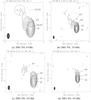 |
Fig. 1 Example of clean images of PKS 1749+096 at 8, 15, 22, and 43 GHz at epoch 2001.701 (2001/09/13). Parameters of the images are given in Table 1. Fitting parameters of the circular Gaussian component are given in Table A.2. |
3. Results
As an example, the final CLEAN images with fitted Gaussian components at 8, 15, 22, and 43 GHz (epoch: 2001.701) are shown in Fig. 1 with detailed parameters of these images presented in Table 1. All resulting CLEAN images and their parameters are presented in Fig. A.1 and Table A.1. In Table A.2 the observation epoch and model-fitting results (including component identification, and model parameters of jet components, such as the flux density, the core separation, the PA, and the size) are summarized.
Description of clean images of PKS 1749+096 shown in Fig. 1.
3.1. Parsec-scale morphology
On parsec scales, PKS 1749+096 showed one-sided extended jet emission to the northeast of the compact VLBI core (Gabuzda et al. 1996; Lobanov et al. 2000; Lu et al. 2007). As shown in Fig. 1, there exist bending jet structures extending to the northeast of the core (Sect. 3.2) that display similar morphology at each frequency at the time of our observations. The extended emission seen at 8 GHz can be detected up to ~8 mas from the core, but it becomes weaker at higher frequencies and is gradually resolved out with increasing resolution. The jet structure is highly core-dominated and, on average, the ratio of core flux to total VLBI flux ( ) is 66.7, 83.0, 88.0, 77.9% at 8, 15, 22 and 43 GHz, respectively.
3.2. Core identification
The two-epoch (1999.348, 2001.701) multi-frequency observations enable us to study the spectra of these VLBI components and then to identify the VLBI core. In Fig. 2 (left), we show the spectra of component D located at the south end of the jet. The spectra of other components are shown in Fig. 2 (right). At 1999.348, component D had a flat spectrum, while at 2001.701, it showed an obvious turnover below 43 GHz, with its optically thin spectrum not measured at this epoch. In addition, component D is also the most compact component based on the modeled size (see Table A.2). Therefore, we identify component D as the compact core of PKS 1749+096. We used the synchrotron self-absorption (SSA) model (Jones et al. 1974) to fit the spectrum of each component, ![Mathematical equation: \begin{equation} S_{\nu}=S_{0}\nu^{2.5}\left[1-\rm exp \left(-\tau_{s}\nu^{\alpha-2.5}\right)\right], \end{equation}](/articles/aa/full_html/2012/08/aa18852-12/aa18852-12-eq26.png) (1)where, ν is the observing frequency in GHz, S0 the intrinsic flux density in Jy at 1 GHz, τs the SSA opacity at 1 GHz, and α the optically thin spectral index. The best-fit results are αD = −0.11 ± 0.07,S0 = 58.4 ± 42.2 mJy,τs = 50.3 ± 46.5 (1999.348), and αD = 0.05 ± 0.01,S0 = 24.6 ± 0.6 mJy,τs = 125.8 ± 7.1 (2001.701). For the first epoch, the accuracy of the fitted parameters is limited by the accuracy of the individual flux density measurements at each frequency and by the limited frequency range of our observations. Jet components show a typically steep spectrum (α ≤ − 0.75) with the exception of C6 (α = −0.3 − -0.2), which may be due to its interaction with the surrounding interstellar medium. The fitted spectral indices for all these components are summarized in Table 2.
(1)where, ν is the observing frequency in GHz, S0 the intrinsic flux density in Jy at 1 GHz, τs the SSA opacity at 1 GHz, and α the optically thin spectral index. The best-fit results are αD = −0.11 ± 0.07,S0 = 58.4 ± 42.2 mJy,τs = 50.3 ± 46.5 (1999.348), and αD = 0.05 ± 0.01,S0 = 24.6 ± 0.6 mJy,τs = 125.8 ± 7.1 (2001.701). For the first epoch, the accuracy of the fitted parameters is limited by the accuracy of the individual flux density measurements at each frequency and by the limited frequency range of our observations. Jet components show a typically steep spectrum (α ≤ − 0.75) with the exception of C6 (α = −0.3 − -0.2), which may be due to its interaction with the surrounding interstellar medium. The fitted spectral indices for all these components are summarized in Table 2.
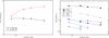 |
Fig. 2 Components’ spectra of PKS 1749+096. Left: spectrum of the core. SSA fits are shown as solid lines. Right: spectra of jet components. |
The magnetic field B of a homogeneous synchrotron self-absorbed source component can be calculated via (i.e., Marscher 1983) (2)here νmax is the peak frequency in GHz, θ the source angular size in mas, Smax the peak flux density in Jy, δ the Doppler factor, and b(α) a tabulated function of the spectral index α. By using Smax = 2.2 Jy and νmax = 11.6 GHz from the above SSA fitting for 1999.348 data and adopting b(α) ≃ 1.8 and θ = θG × 1.8 mas, where θG is the fitted-Gaussian FWHM and the factor of 1.8 accounts for the Gaussian approximation to an optically thin uniform sphere, we obtained Bsyn = 3.9 × 10⁻²δ mG.
Results of spectral fitting for jet components of PKS 1749+096.
Assuming the energy equipartition between the radiative particles and magnetic field, one can also estimate the magnetic field using the synchrotron luminosity L. The energy of the particles can be written as  (3)where,
  , f(α,ν1,ν2) is a tabulated function, ν1 and ν2 are the low and high cutoff frequency of normally 107 and 1011 Hz, respectively (Pacholczyk 1970). In the case of spherical symmetry, the energy density of the magnetic field is
  , and the magnetic field energy of a source (with radius R) is
  (4)If the energy ratio of heavy particles to electrons is η, then the total energy can be expressed as
 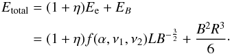 (5)η is determined by the matter content of the jet, and in an electron-positron pair plasma, η ≈ 1, while in a “normal” electron-proton plasma, η ≈ 2000. It seems to be reasonable to adopt η = 100 (Pacholczyk 1970). Note that
  and EB ∝ B2, so the total energy Etotal has a minimum, and in this case, the magnetic filed is
 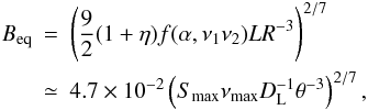 (6)where
  , f(−0.11,107,1011) = 0.74 × 10⁷, and DL is the luminosity distance in Gpc. Using the same parameters for deriving Bsyn, we obtain Beq = 0.8 G. This is much larger than that derived from SSA, indicating that either the radiation is strongly Doppler-boosted or that the source is particle-dominated. In the former case, since Bsyn and Beq depend differently on the Doppler factor δ (cf. Eqs. (2) and (6)), one obtains
  (e.g., Feng et al. 2006). Correspondingly, the derived Doppler factor is the equipartition Doppler factor δeq, and for the core component D, we obtain
  . In this case, we get Bsyn = 0.2 mG, which seems to be a low value for an AGN jet. In the latter case, the ratio of energy density in particles (up) to magnetic field (um) can be written as
  , according to Readhead (1994). Thus, we obtain
  (ignoring relativistically beaming effect), indicating that the core is strongly particle-dominated.
3.3. Jet kinematics
3.3.1. 22 GHz
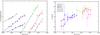 |
Fig. 3 Core separation (left) and PA (right) of jet components plotted as a function of time at 22 GHz. The solid lines represent linear fits (left, see Table 3). C5 is not shown to obtain a clear plot for the inner jet components. |
To study the jet kinematics, we show in Fig. 3 (left) the core separation as a function of time along with the linear regression fits through which the apparent speeds of the individual jet components are measured. The fitted results are summarized in Table 3. Figure 3 (right) plots the time evolution of the PA of jet components. As a result seven components (C5–C11) are identified at 22 GHz. However, the identification of C9 is possibly subject to some uncertainties because of the time gaps during 2003–2004. All these components move away from the core, with proper motion in the range of 0.25–1.05 mas/yr, corresponding to apparent speeds of 5–21 c. Interestingly, the apparent speeds seem to follow a bimodal distribution. C9, C10, and C11 move 2–3 times faster than the other components (C5, C6, C7, and C8). It can be seen from Fig. 3 (right) that the PAs for most jet components show no significant variations. The averages of the PAs for these components are summarized in Table 3, too. One exception is for component C7, whose PA systematically varies with time. A discussion of this result is deferred to the following section.
Results of the linear fits to the component motion at 22 GHz.
3.3.2. 15 GHz
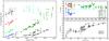 |
Fig. 4 Core separation (left) and PA (right) of jet components plotted as a function of time at 15 GHz. The solid lines represent linear fits (see Table 4). The PAs of C1, C2, and C4 are shifted for a better visualization (upper right). |
Results of the linear fits to the component motion at 15 GHz.
In view of the bimodal distribution of apparent jet speeds at 22 GHz and the “mode” switch for jet kinematics in some BL Lac objects (Britzen et al. 2010b), we then considered the 15 GHz MOJAVE data with relatively longer time coverage. However, the irregular time sampling (e.g., gaps around 1998–1999 and 2005) and the complexity of the jet kinematics make it nearly impossible to trace all the jet components. We therefore turned to investigate a few features for which we were able to follow the evolution during the studied period to obtain the main characteristics of the jet kinematics. Figure 4 (left) shows the core distance evolution of the modeled components with obvious proper motion at 15 GHz together with the linear regression fit. Table 4 summarizes the fitting results. These components show similar speeds, and for component C5 and C7, the fitted speeds and ejection time at 15 and 22 GHz are consistent (Tables 3 and 4), considering the different time coverage and data points at each frequency. For component C6, the core separation does not increase linearly with time and therefore a linear regression was not considered. Iguchi et al. (2000) measured the proper motion of component C5 (C1 in their case) 0.68 ± 0.14 mas yr-1. Based on the data of three epochs, the inferred ejection time of May 1997 is slightly later than what we derived for component C5 (1996.9). Iguchi et al. (2000) deduced that the core contained an unresolved component extending to the northwest along a PA of ~−30° during their observations in 1998. It turns out that this component can be identified as component C6 from our analysis (Table A.2). Although bearing relatively large uncertainties because of the limited data (three epochs) at 22 GHz, the ejection time (around 1999) and PA (along ~ −30°) of component C6 are identical to the unresolved component. This component was also detected by space-based VLBI at 5 GHz (epoch: 2001.24 Gabuzda 2003). Homan et al. (2001) reported a proper motion of 0.45 mas/yr for component C4 (their U3) based on the data of six epochs in 1996, which is slightly faster than our estimated speed of 0.29 mas/yr. They considered that the position of this component was affected by the strong core in some epochs. Similarly, this effect at 1997.658 may also explain the relatively low speed. In addition, Lister et al. (2009b) reported a maximum apparent speed of 6.8 c in PKS 1749+096.
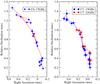 |
Fig. 5 Trajectory of the components C6 an C7 in the sky plane. |
In Fig. 4 (right) we show the time evolution of the PA of jet components. Most components keep nearly constant PA when they move downstream of the jet. The average PAs for these components are given in Table 4. Obviously, C6 and C7 are two exceptions with their PAs showing systematic variations with time. In Fig. 5, the trajectories of component C6 and C7 in the sky plane are displayed, which exhibits a clear non-radial, non-ballistic motion.
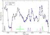 |
Fig. 6 Light curves of PKS 1749+096 from total VLBI flux density data (filled circles) and single-dish flux density data (open circles, UMRAO data) at 15 GHz. The fitted component ejection time is indicated by the vertical lines, whose length is proportional to the flux density of each component (C4–C7: 15 GHz, C8–C11: 22 GHz) when first seen. Horizontal bars along the time axis denote the uncertainty of the ejection time of each labeled component. |
In many AGN, radio outbursts are believed to be connected with VLBI component ejections (e.g., Savolainen et al. 2002). Figure 6 shows the evolution of the UMRAO total flux density (open circles) and of the VLBI total flux density (filled circles) at 15 GHz. The agreement of these two quantities demonstrates the reliability of the VLBI amplitude calibration. In Fig. 6, the fitted ejection time for components C4–C11 is also marked. Evidently, the ejection of jet components is connected with the radio outbursts, even though not all events are linked in a similar manner (e.g., C5 and C8 appear to be ejected early in the rise phase of the flux density), as indicated by the data. Given the time coverage of the available data, and because acceleration/deceleration could affect the linear back-extrapolation of the ejection time when the component is coincident with the core, it is hard to accurately estimate the time difference between the ejection of a component and the outburst from these data. By considering that there are about 10 years of total flux density measurements and a time window of, on average, about 0.31 yr, within which the flare peaks and component ejections would be considered as related, we estimate the probability that all eight events are connected by chance is ~3.4 × 10⁻⁶. Therefore, we conclude that, at least in PKS 1749+096, there exists correlation between the emergency of VLBI components and radio outbursts.
Also shown in Fig. 6 are the normalized flux density (relative to C6) of each component when they were detected by our observations for the first time. It is interesting to note that the strength of the outburst seems to be correlated with the component brightness (e.g., C9). However, since components are typically not first detected at the same core distance and they may evolve differently with time, they cannot be readily put into one-to-one correspondence (e.g., C10 and C11). Nieppola et al. (2009) studied multi-frequency (5, 8, 15, 22, 37, and 90 GHz) radio light curves of PKS 1749+096, and identified five major outbursts, peaked in 1993, 1995, 1998, 2001, and 2002. These outbursts correspond to the ejection time of components C3, C4, C6, C7, and C82, respectively.
3.4. The component C5
Component C5 is the most reliably determined feature by the data. In Fig. 7, we plot its 15 GHz flux density as a function of time. The flux density of C5 shows a rapid decrease after its birth until it reaches a flux density of ~20 mJy in 2002 at 15 GHz. In contrast, the total flux density of PKS 1749+096 (see Fig. 6) during this period does not show such a monotonic behavior, but instead shows three major flares. The rate of the flux density decay of C5 slows down as it moves outward, and the evolution can be described reasonably well by a power law of the form of S(t) ~ (t − t0)κ with t0 = 1995.45 ± 0.01 and κ = −2.97 ± 0.07, which is indicated as a solid line in Fig. 7.
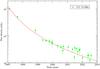 |
Fig. 7 Flux density evolution of component C5 at 15 GHz. The solid line represents a power-law fit. See text for details. |
In Fig. 8, we show the spectrum of C5 determined by simultaneous multi-frequency observations in 1998 (Iguchi et al. 2000), 1999, and 2001, respectively. The spectral indices are − 0.71 ± 0.053 in 1998.849, − 0.75 ± 0.09 in 1999.348, and − 1.28 ± 0.21 in 2001.701, showing that the spectrum steepens with time at a probability of 97%. An analysis of multi-frequency (2.3, 8.4, 15.3, 22,2 and 43 GHz) VLBA data on May 12, 2001 (epoch 2001.362, code: BW055) yields a spectral index of − 1.17 ± 0.10 and additionally confirms the spectral steepening for component C5.
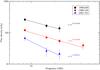 |
Fig. 8 Spectral evolution of component C5. The solid lines represent power-law fits. |
Components showing monotonic decrease in flux density as they move outward from the core have been observed in a number of sources (e.g., 3C 345,0735+178, Unwin et al. 1983; Gabuzda et al. 1994a,b). The flux density evolution can be basically explained in terms of geometric Doppler boosting effects and intrinsic effects as the result of radiation or adiabatic expansion loss.
In the former case, the observed flux density (S) of a component is related to the intrinsic flux density (S0) in the comoving frame by S = S0δ3 − α (Scheuer & Readhead 1979). This formula indicates that the geometric effect is frequency-independent. The steepening of the spectra, as shown in Fig. 8, indicates the frequency-dependent behavior of flux density evolution for component C5. Furthermore, the trajectory needs to be sharply curved to explain the changes in flux density, which is inconsistent with the observed ballistic trajectory (Sect. 3.3.2).
In the latter case, a simple adiabatic expansion predicts S(t) ~ (t − t0)κ, with κ = 4α − 2 (Kardashev 1962) and would maintain a constant spectral index (van der Laan 1966). For the fitted power law index of κ = −2.97 ± 0.07, α = −0.24 ± 0.02, which is flatter than the measured indices. The fitted t0 is earlier than the extrapolated time of ejection from kinematics, indicating that the expansion may begin with a finite flux density, instead of infinity. A plausible alternative could be adiabatic expansion with a continuous acceleration of the energy index 2α − 1. This would lead to κ = 2α − 1 (Kardashev 1962) and α = −0.98 ± 0.04, which roughly matches the measured spectral indices within errors.
The spectral steepening as seen in Fig. 8 is reminiscent of radiation losses. Following Eq. (2), we estimate the magnetic field strength to be Bsyn = 268 mG adopting νmax = 2.37 GHz, θ = 2.52 mas, Smax = 0.90 Jy, b(α) = 3.6 and δeq = 2.5 (Iguchi et al. 2000). The cooling time  of synchrotron-emitting electrons follows
  , where is in years, Bsyn in mG, and νmax in GHz. This yields
  years for component C5, comparable to the time scale of flux density evolution. The estimated equipartition Doppler factor δeq of 2.5 indicates
  . This perhaps means that C5 is particle-dominated and the inverse Compton scattering also contributes to the fast decrease in flux density of C5.
3.5. Physical parameters
One can estimate the physical parameters of the parsec-scale jet using the measured apparent speeds. C5 (βapp = 10.2 c) is the best-determined component in our experiments with as many as 25 data points, and therefore will be used in the following calculations. The Doppler factor (δ) is determined by the Lorentz factor Γ, the viewing angle of the jet θ, and the jet speed in the source frame β:  (7)where
  The maximum allowable viewing angle θmax can be derived via
  (8)and the minimum Lorentz factor is given by
  (9)For component C5, θmax = 11.2°, Γmin = 10.2. For a given speed in the source frame, β, the critical viewing angle, which maximizes the apparent speed, is given by
  . θcri = 5.6° for component C5. According to Eq. (7), the minimum Lorentz factor Γmin and the critical viewing angle θcri lead to δ = Γmin = 10.2. This indicates that the Doppler factor of component C5 is close to that of the core component D (
 ). For even smaller viewing angles (θ → 0), Doppler factor approaches ~2Γ = 20.4.
4. Discussion
4.1. Structure variability
In Fig. 9, we plot the PA distribution as a function of core separation at 15 and 22 GHz. To distinguish the ambiguity of measurement errors near the core, we also plot within each core separation bin the scatter of jet PA with comparison to the typical measurement errors derived from the often quoted 1/5 of the beam size, which we took to be 0.5 mas for these measurements, with most taken at 15 GHz (Fig. 9, inset). Clearly, the scatter of the PA in each bin is always larger than the typical errors, and therefore there is no fixed trajectory that all the jet components can follow within the central ~4−6 mas. It should be noted that the time sampling of these observations is not equal (e.g., there were seven epochs in 1996, but only one epoch in 1998). In view of this, Fig. 10 displays the time evolution of the jet ridge line (defined as the line connecting the modeled jet components), which clearly shows the change of the PA.
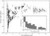 |
Fig. 9 Position angle plotted as a function of core separation for all jet components seen at 15 (open) and 22 GHz (filled). The inset histogram is a plot of the scatter of PAs (shaded) in each bin (0.5 mas) with comparison to the errors (blank) from the often quoted 1/5 of the beam size (see text for details). |
From Tables 3 and 4, it is obvious that the jet components were ejected at various PAs, and this is particularly true for components C6 and C7. Indeed, dramatic jet-ejection-angle variation is not uncommon in many AGNs (e.g., in PKS 0048-097, Kadler et al. 2006), and a precessing jet scenario is often cited as the explanation. The jet precession can be triggered either by a binary black hole system or by a warped accretion disk. A simple scenario is a precessing ballistic jet where jet components ejected at different times move ballistically to different directions (e.g., Stirling et al. 2003). A jet precession would lead to the change of the inner jet structure and of the component ejection angle, which was indeed observed in PKS 1749+096. However, these ejection angles are distributed in a random rather than systematic manner, and therefore do not appear to be consistent with a precessing jet scenario. On the other hand, the variation timescale of the jet ejection angle seems to be much shorter than the precession period (Lobanov & Roland 2005).
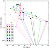 |
Fig. 10 Time evolution of jet ridge line at 15 GHz. Only one epoch is shown for each year for clarity. |
4.2. Kinematics of BL Lac objects
Britzen et al. (2010b) recently pointed out that BL Lac objects differ appreciably in the parsec-scale jet kinematics from quasars. According to these authors, the jet kinematics in BL Lac objects cannot always be described by the standard AGN paradigm of apparent superluminal motion. Instead, there exists structural mode change, i.e., transition from “typical superluminal” to an unusual “stationary” state. For PKS 1749+096, a similar mode change is not found. The reason could be that the time coverage of the observations is not long enough. In contrast, we found that there is a bimodal distribution of apparent superluminal speeds and there coexist ballistic and non-ballistic components, which caused the bending of the jet. Kudryavtseva et al. (2011) also detected a component similar to components C6 and C7 in the quasar B0605-085 and attributed this to jet precession. However, the reasons for the existence of a bimodal distribution of apparent speeds and whether this bimodality has any correlation with other properties of the jet, such as the flux density evolution, are unclear. It is not readily obvious that the kinematic behavior of the pc-scale jet is simply a result of a changing viewing angle of the jet. The flux density evolution shows nothing special that could be linked to the sources of each bimodal population, which is complicated by the fact that most, if not all, of the outbursts are connected with the ejection of jet components.
The apparent jet speeds of BL Lac objects are generally lower than those of quasars, typically ≤ 5 c (Jorstad et al. 2001; Hovatta et al. 2009). Our observations suggest that the jet in PKS 1749+096 moves faster than in other BL Lac objects with an average apparent jet speed of ~9 c and with some components moving as fast as 21 c. In this sense, PKS 1749+096 is an unusual BL Lac object, showing superluminal speeds similar to quasars (~10–20 c).
5. Summary
We studied the parsec-scale jet of PKS 1749+096 by using high-resolution multi-epoch (total of 65 observations in 61 epochs spanning ~10 years) VLBI observations at 8, 15, 22, and 43 GHz. On parsec scales, PKS 1749+096 showed a core-jet structure with the jet extending to the northeast. The compact core contains, on average, ~80% of the total VLBI flux density. Using two-epoch (1999.348 and 2001.701) multi-frequency simultaneous observations, we identified the component D as the VLBI core based on its flat spectrum and compactness. The derived equipartition Doppler factor for the core was found to be consistent with the Doppler factor of jet component (C5) estimated from kinematics. We found that models of adiabatic expansion or Doppler boosting cannot solely account for the flux density decay of component C5. Although the synchrotron cooling time scale is comparable to the decay time scale, this component was probably far away from energy equipartition and was dominated by particles. The fast decay of flux density may be caused partly by inverse Compton scattering effects in addition to the expansion.
The study of the jet kinematics shows that the components exhibited a bimodal distribution of superluminal speeds in PKS 1749+096, i.e., C9, C10, and C11’s proper motions are faster than that of other components. The available evidence shows that ballistic and non-ballistic components coexisted, though the cause for this is still unclear. The superluminal motion of jet components is in the range of 5–21 c. In PKS 1749+096, the component ejection correlates in time with radio flux density outburst, supporting the commonly assumed connection between the two.
Online material
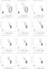 |
Fig. A.1 Clean images of PKS 1749+096. |
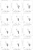 |
Fig. A.1 continued. |
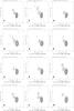 |
Fig. A.1 continued. |
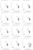 |
Fig. A.1 continued. |
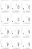 |
Fig. A.1 continued. |
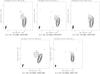 |
Fig. A.1 continued. |
Description of VLBA images of PKS 1749+096 shown in Fig. A.1.
Model-fitting results for PKS 1749+096.
Note that the position of C8 may be affected by C9 at epoch 2003.216, when C9 was unresolved from the core, we therefore consider that the ejection time of C8 (2001.5) corresponds to the outburst in 2002.
Iguchi et al. (2000) obtained a spectral index of −0.98 ± 0.05 on the basis of non-simultaneous data.
Acknowledgments
We thank the referee for the useful comments and suggestions. The Very Long Baseline Array is a facility of the National Radio Astronomy Observatory, USA, operated by Associated Universities Inc., under cooperative agreement with the National Science Foundation. This research has made use of data from the MOJAVE database that is maintained by the MOJAVE team (Lister et al. 2009a). The authors thank M. Aller for providing UMRAO data, partly prior to publication. UMRAO is supported by the National Science Foundation under a series of grants, most recently AST-0607523, and by funds from the University of Michigan. Special thanks are due to T. Savolainen for providing data that were used for spectral analysis. This work is also based on observations with the 100-m telescope of the MPIfR (Max-Planck-Institut für Radioastronomie) at Effelsberg. Z.Q.S. acknowledged the support by China Ministry of Science and Technology under State Key Development Program for Basic Research (2012CB821800), the National Natural Science Foundation of China (grants 10625314, 10821302 and 11173046), and the CAS/SAFEA International Partnership Program for Creative Research Teams.
References
- Abdo, A. A., Ackermann, M., Ajello, M., et al. 2009, ApJ, 700, 597 [NASA ADS] [CrossRef] [Google Scholar]
- Britzen, S., Kudryavtseva, N. A., Witzel, A., et al. 2010a, A&A, 511, A57 [NASA ADS] [CrossRef] [EDP Sciences] [Google Scholar]
- Britzen, S., Witzel, A., Gong, B. P., et al. 2010b, A&A, 515, A105 [NASA ADS] [CrossRef] [EDP Sciences] [Google Scholar]
- Dallacasa, D., Stanghellini, C., Centonza, M., & Fanti, R. 2000, A&A, 363, 887 [NASA ADS] [Google Scholar]
- Fan, J. H., & Lin, R. G. 1999, ApJS, 121, 131 [NASA ADS] [CrossRef] [Google Scholar]
- Feng, S., Shen, Z., Cai, H., et al. 2006, A&A, 456, 97 [NASA ADS] [CrossRef] [EDP Sciences] [Google Scholar]
- Fomalont, E. B. 1999, in Synthesis Imaging in Radio Astronomy II, eds. G. B. Taylor, C. L. Carilli, & R. A. Perley, ASP, Conf. Ser., 180, 301 [Google Scholar]
- Gabuzda, D. C. 2003, in High Energy Blazar Astronomy, eds. L. O. Takalo, & E. Valtaoja, ASP, Conf. Ser., 299, 99 [Google Scholar]
- Gabuzda, D. C., Mullan, C. M., Cawthorne, T. V., Wardle, J. F. C., & Roberts, D. H. 1994a, ApJ, 435, 140 [NASA ADS] [CrossRef] [Google Scholar]
- Gabuzda, D. C., Wardle, J. F. C., Roberts, D. H., Aller, M. F., & Aller, H. D. 1994b, ApJ, 435, 128 [NASA ADS] [CrossRef] [Google Scholar]
- Gabuzda, D. C., Sitko, M. L., & Smith, P. S. 1996, AJ, 112, 1877 [NASA ADS] [CrossRef] [Google Scholar]
- Gabuzda, D. C., Pushkarev, A. B., & Cawthorne, T. V. 1999, MNRAS, 307, 725 [NASA ADS] [CrossRef] [Google Scholar]
- Homan, D. C., Ojha, R., Wardle, J. F. C., et al. 2001, ApJ, 549, 840 [NASA ADS] [CrossRef] [Google Scholar]
- Hovatta, T., Valtaoja, E., Tornikoski, M., & Lähteenmäki, A. 2009, A&A, 494, 527 [NASA ADS] [CrossRef] [EDP Sciences] [Google Scholar]
- Iguchi, S., Fujisawa, K., Kameno, S., et al. 2000, PASJ, 52, 1037 [NASA ADS] [Google Scholar]
- Jones, T. W., O’dell, S. L., & Stein, W. A. 1974, ApJ, 192, 261 [NASA ADS] [CrossRef] [Google Scholar]
- Jorstad, S. G., Marscher, A. P., Mattox, J. R., et al. 2001, ApJS, 134, 181 [NASA ADS] [CrossRef] [Google Scholar]
- Kadler, M., Hughes, P. A., Ros, E., Aller, M. F., & Aller, H. D. 2006, A&A, 456, L1 [NASA ADS] [CrossRef] [EDP Sciences] [Google Scholar]
- Kardashev, N. S. 1962, Soviet Ast., 6, 317 [Google Scholar]
- Kellermann, K. I., Lister, M. L., Homan, D. C., et al. 2004, ApJ, 609, 539 [NASA ADS] [CrossRef] [Google Scholar]
- Krichbaum, T. P., Graham, D. A., Greve, A., et al. 1997, A&A, 323, L17 [Google Scholar]
- Kudryavtseva, N. A., Britzen, S., Witzel, A., et al. 2011, A&A, 526, A51 [NASA ADS] [CrossRef] [EDP Sciences] [Google Scholar]
- Lister, M. L., & Homan, D. C. 2005, AJ, 130, 1389 [NASA ADS] [CrossRef] [Google Scholar]
- Lister, M. L., Aller, H. D., Aller, M. F., et al. 2009a, AJ, 137, 3718 [NASA ADS] [CrossRef] [Google Scholar]
- Lister, M. L., Cohen, M. H., Homan, D. C., et al. 2009b, AJ, 138, 1874 [NASA ADS] [CrossRef] [Google Scholar]
- Lobanov, A. P., & Roland, J. 2005, A&A, 431, 831 [NASA ADS] [CrossRef] [EDP Sciences] [Google Scholar]
- Lobanov, A. P., Krichbaum, T. P., Graham, D. A., et al. 2000, A&A, 364, 391 [NASA ADS] [Google Scholar]
- Lu, R., Shen, Z., Krichbaum, T. P., et al. 2007, in The Central Engine of Active Galactic Nuclei, eds. L. C. Ho, & J.-M. Wang, ASP Conf. Ser., 373, 237 [Google Scholar]
- Marscher, A. P. 1983, ApJ, 264, 296 [NASA ADS] [CrossRef] [Google Scholar]
- Mattox, J. R., Hartman, R. C., & Reimer, O. 2001, ApJS, 135, 155 [NASA ADS] [CrossRef] [Google Scholar]
- Nieppola, E., Hovatta, T., Tornikoski, M., et al. 2009, AJ, 137, 5022 [NASA ADS] [CrossRef] [Google Scholar]
- Pacholczyk, A. G. 1970, Radio astrophysics. Nonthermal processes in galactic and extragalactic sources, Series of Books in Astronomy and Astrophysics (San Francisco, CA: Freeman) [Google Scholar]
- Readhead, A. C. S. 1994, ApJ, 426, 51 [Google Scholar]
- Rector, T. A., & Stocke, J. T. 2003, AJ, 125, 2447 [NASA ADS] [CrossRef] [Google Scholar]
- Savolainen, T., Wiik, K., Valtaoja, E., Jorstad, S. G., & Marscher, A. P. 2002, A&A, 394, 851 [NASA ADS] [CrossRef] [EDP Sciences] [Google Scholar]
- Scheuer, P. A. G., & Readhead, A. C. S. 1979, Nature, 277, 182 [NASA ADS] [CrossRef] [Google Scholar]
- Stickel, M., Fried, J. W., & Kuehr, H. 1988, A&A, 191, L16 [NASA ADS] [Google Scholar]
- Stirling, A. M., Cawthorne, T. V., Stevens, J. A., et al. 2003, MNRAS, 341, 405 [NASA ADS] [CrossRef] [Google Scholar]
- Torniainen, I., Tornikoski, M., Teräsranta, H., Aller, M. F., & Aller, H. D. 2005, A&A, 435, 839 [NASA ADS] [CrossRef] [EDP Sciences] [Google Scholar]
- Unwin, S. C., Cohen, M. H., Pearson, T. J., et al. 1983, ApJ, 271, 536 [NASA ADS] [CrossRef] [Google Scholar]
- van der Laan, H. 1966, Nature, 211, 1131 [NASA ADS] [CrossRef] [Google Scholar]
All Tables
All Figures
|
Fig. 1 Example of clean images of PKS 1749+096 at 8, 15, 22, and 43 GHz at epoch 2001.701 (2001/09/13). Parameters of the images are given in Table 1. Fitting parameters of the circular Gaussian component are given in Table A.2. |
| In the text | |
|
Fig. 2 Components’ spectra of PKS 1749+096. Left: spectrum of the core. SSA fits are shown as solid lines. Right: spectra of jet components. |
| In the text | |
|
Fig. 3 Core separation (left) and PA (right) of jet components plotted as a function of time at 22 GHz. The solid lines represent linear fits (left, see Table 3). C5 is not shown to obtain a clear plot for the inner jet components. |
| In the text | |
|
Fig. 4 Core separation (left) and PA (right) of jet components plotted as a function of time at 15 GHz. The solid lines represent linear fits (see Table 4). The PAs of C1, C2, and C4 are shifted for a better visualization (upper right). |
| In the text | |
|
Fig. 5 Trajectory of the components C6 an C7 in the sky plane. |
| In the text | |
|
Fig. 6 Light curves of PKS 1749+096 from total VLBI flux density data (filled circles) and single-dish flux density data (open circles, UMRAO data) at 15 GHz. The fitted component ejection time is indicated by the vertical lines, whose length is proportional to the flux density of each component (C4–C7: 15 GHz, C8–C11: 22 GHz) when first seen. Horizontal bars along the time axis denote the uncertainty of the ejection time of each labeled component. |
| In the text | |
|
Fig. 7 Flux density evolution of component C5 at 15 GHz. The solid line represents a power-law fit. See text for details. |
| In the text | |
|
Fig. 8 Spectral evolution of component C5. The solid lines represent power-law fits. |
| In the text | |
|
Fig. 9 Position angle plotted as a function of core separation for all jet components seen at 15 (open) and 22 GHz (filled). The inset histogram is a plot of the scatter of PAs (shaded) in each bin (0.5 mas) with comparison to the errors (blank) from the often quoted 1/5 of the beam size (see text for details). |
| In the text | |
|
Fig. 10 Time evolution of jet ridge line at 15 GHz. Only one epoch is shown for each year for clarity. |
| In the text | |
|
Fig. A.1 Clean images of PKS 1749+096. |
| In the text | |
|
Fig. A.1 continued. |
| In the text | |
|
Fig. A.1 continued. |
| In the text | |
|
Fig. A.1 continued. |
| In the text | |
|
Fig. A.1 continued. |
| In the text | |
|
Fig. A.1 continued. |
| In the text | |
Current usage metrics show cumulative count of Article Views (full-text article views including HTML views, PDF and ePub downloads, according to the available data) and Abstracts Views on Vision4Press platform.
Data correspond to usage on the plateform after 2015. The current usage metrics is available 48-96 hours after online publication and is updated daily on week days.
Initial download of the metrics may take a while.