| Issue |
A&A
Volume 543, July 2012
|
|
|---|---|---|
| Article Number | A110 | |
| Number of page(s) | 14 | |
| Section | The Sun | |
| DOI | https://doi.org/10.1051/0004-6361/201219311 | |
| Published online | 06 July 2012 | |
The standard flare model in three dimensions
I. Strong-to-weak shear transition in post-flare loops
LESIA, Observatoire de Paris, CNRS, UPMC, Univ. Paris Diderot, 5 place Jules Janssen, 92190 Meudon, France
e-mail: This email address is being protected from spambots. You need JavaScript enabled to view it.
Received: 30 March 2012
Accepted: 20 May 2012
Abstract
Context. The standard CSHKP model for eruptive flares is two-dimensional. Yet observational interpretations of photospheric currents in pre-eruptive sigmoids, shear in post-flare loops, and relative positioning and shapes of flare ribbons, all together require three-dimensional extensions to the model.
Aims. We focus on the strong-to-weak shear transition in post-flare loops, and on the time-evolution of the geometry of photospheric electric currents, which occur during the development of eruptive flares. The objective is to understand the three-dimensional physical processes, which cause them, and to know how much the post-flare and the pre-eruptive distributions of shear depend on each other.
Methods. The strong-to-weak shear transition in post-flare loops is identified and quantified in a flare observed by STEREO, as well as in a magnetohydrodynamic simulation of CME initiation performed with the OHM code. In both approaches, the magnetic shear is evaluated with field line footpoints. In the simulation, the shear is also estimated from ratios between magnetic field components.
Results. The modeled strong-to-weak shear transition in post-flare loops comes from two effects. Firstly, a reconnection-driven transfer of the differential magnetic shear, from the pre- to the post-eruptive configuration. Secondly, a vertical straightening of the inner legs of the CME, which induces an outer shear weakening. The model also predicts the occurrence of narrow electric current layers inside J-shaped flare ribbons, which are dominated by direct currents. Finally, the simulation naturally accounts for energetics and time-scales for weak and strong flares, when typical scalings for young and decaying solar active regions are applied.
Conclusions. The results provide three-dimensional extensions to the standard flare model. These extensions involve MHD processes that should be tested with observations.
Key words: magnetic reconnection / magnetohydrodynamics (MHD) / Sun: coronal mass ejections (CMEs) / Sun: flares / Sun: UV radiation
© ESO, 2012
1. Introduction
Solar flares are among the most energetic events of the solar system. Their frequent association with coronal mass ejections (CMEs, see e.g. Schrijver et al. 2011) and with solar energetic particles (SEPs, see e.g. Masson et al. 2009) makes them among the most intense drivers of space weather. While they emit in the whole range of the electromagnetic spectrum, their radiative increase is the largest in the extreme ultraviolet (EUV) and in soft X-rays (SXR), both of which originate from chromospheric ribbons (see e.g. Schmieder et al. 1987; del Zanna et al. 2006) and coronal post-flare loops (see e.g. Schmieder et al. 1995; Warren et al. 2011).
The formation of flare ribbons and flare loops (also historically referred to as post-flare loops, which we use hereafter) has been explained since a long time in the framework of a series of cartoons, which are now referred to as the standard model (or the CSHKP model, named after Carmichael 1964; Sturrock 1966; Hirayama 1974; Kopp & Pneuman 1976). The latter is essentially two-dimensional. It states that post-flare loops are formed by coronal magnetic reconnection, which develops in a vertical current sheet located between two oppositely oriented magnetic fields (Lin & Forbes 2000), and that the ribbons are heated by energy transport from the coronal reconnection site. For eruptive flares, the vertical magnetic fields on both sides of the current sheet correspond to the legs of CME-related expanding field lines (see e.g. Forbes et al. 2006; Aulanier et al. 2010, for reviews about triggering CMEs). Several 2.5D MHD simulations for flares and CME early phases have calculated the magnetic and thermal properties of this standard model (e.g. Amari et al. 1996; Chen & Shibata 2000; Linker et al. 2003; Reeves & Forbes 2005; Shiota et al. 2005; Jacobs et al. 2006). They confirmed the cartoons, and successfully explained many observed properties. We refer the reader to the recent review by Shibata & Magara (2011), for a complete description of these findings.
Multi-wavelength observations of flares, however, also exhibit many three-dimensional features. Among those are coronal sigmoids (e.g. Aulanier et al. 2010; Green et al. 2011; Savcheva et al. 2012), erupting flux ropes (e.g. Zhang et al. 2012), and bright footpoint emissions moving along ribbons as seen in HXR (e.g. Fletcher & Hudson 2002) and in the EUV (del Zanna et al. 2006; Chandra et al. 2009). In addition, observations fequently show that post-flare loops exhibit a clear gradual transition from a sheared to a nearly potential configuration. This transition, which seems to occur at different rates for different flares, has rarely been explicitly mentioned. Nevertheless, it clearly manifests itself in many EUV observations: offsets of chromospheric ribbons from one another, along the polarity inversion line (PIL), can be seen in Chandra et al. (2009) and Wang et al. (2012); varying shear angles of segments joining pairs of bright kernels, within chromospheric ribbons, were measured in Asai et al. (2003) and in Su et al. (2006, 2007); varying shear angles of EUV and visible coronal post-flare loops can be seen in Asai et al. (2003, Fig. 4), Liu et al. (2010, Fig. 2, online movie), Inoue et al. (2011, Figs. 2 and 3), Warren et al. (2011, Fig. 3) and Savage et al. (2012, Fig. 2).
Unfortunately, neither the third dimension nor the shear is considered in the CSHKP model. So the standard model remains insufficient to explain these observations. Several 3D models have been recently proposed in the form of cartoons (Shibata et al. 1995; Moore et al. 2001; Priest & Forbes 2002). Unlike the standard model in 2D, these cartoons have been successful in explaining many of the aforementioned observed features. But these cartoons still do not address the physical processes at work in generating electric currents and magnetic shear within chromospheric ribbons and coronal post-flare loops. New analyses of realistic 3D MHD simulations for eruptive flares are therefore required, so as to provide physical interpretations to the observations.
Regarding the strong-to-weak shear transition in post-flare loops in particular, competing interpretations were put forward due to the lack of a comprehensive standard flare model in 3D: Asai et al. (2003) attributed it to the emergence of a twisted flux tube from below the photosphere; Su et al. (2006) sketched it as a sequential reconnection-driven transfer of the shear distribution from within and around the pre-erupting flux rope, into the post-flare loops; Inoue et al. (2011) found that the shear and twist actually increase early in their flare, with a dispersal in their estimations suggesting that the shear might eventually weakly decrease at late times.
The general objective of this paper is to extend the standard flare model in three dimensions, so as to use it for modeling real flares observed at the Sun. Specifically, the paper focuses on the nature and timing of the strong-to-weak shear transition in post-flare loops, through the analyses of space observations and of a numerical simulation. It also addresses the development of electric currents in the photosphere.
This paper is organized as follows. Section 2 contains the analysis of the post-flare loops that develop during one specific eruptive flare, as observed by STEREO and SDO. Section 3 describes the setup of a generic 3D numerical simulation for solar eruptions, that can be applied to observations, which we perform with the OHM code. Section 4 reports on the general properties of the simulated CME and flare, on their comparison with the CSHKP model, and on their energetics and time-scales. Section 5 contains the analysis of the time-evolution of the geometry of the reconnecting field lines, and of various shear angle proxies which unveil the physical origins of the strong-to-weak shear transition in post-flare loops. This analysis also leads to describe the shapes and time-evolutions of photospheric electric currents within flare ribbons and sunspots. Section 6 summarizes the results.
2. Case-study of an observed eruptive flare
2.1. Selection of the studied event
Several observational proxies can be used to quantify the strong-to-weak shear transition in post-flare loops. Asai et al. (2003) and Su et al. (2006) considered pairs of connected kernels located inside flare ribbons (the latter could not observe the post-flare loops, but they performed very careful identifications of the pairs of kernels). Inoue et al. (2011) considered the mean observed currents at the footpoints of field lines calculated with a sequence of force-free extrapolations. Here, we analyze an event for which we can use the footpoints of the observed post-flare loops themselves, as a proxy.
We chose our event so as to satisfy the following six criteria: (i) an isolated bipolar region (to avoid any physical interference from neighboring flux concentrations); (ii) a smooth and weakly curved polarity inversion line (or PIL, to avoid introducing amibiguities in the shear angle mesurements); (iii) a flare observed almost face-on (to limit projection effects which can affect the identification of individual loops); (iv) a flare of moderate energy (to avoid intensity saturation and leaking within the post-flare loops); (v) a long time-scale for the strong-to-weak shear transition (to be able to measure the angle variation with time); (vi) an active region which is not continuously subject to shearing motions (to avoid the effect of photospheric motions in generating shear in the corona).
We revisited the same flares which showed the strong-to-weak shear transition in post-flare loops as found in the references listed in Sect. 1, and we reviewed those which satisfied our criteria. The two best candidates were C-class flares, originating from decaying active regions (ARs) located in the northern hemisphere, and associated with sigmoid eruptions: the August 1, 2010 flare (Liu et al. 2010) and the May 9, 2011 flare (Warren et al. 2011). We chose the latter, as its bipolar magnetic field environment was more symmetric than the former.
2.2. The May 9, 2011 event observed by EUVI and HMI
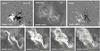 |
Fig. 1 SDO/HMI and STEREO-B/EUVI observations of the May 9, 2011 eruptive flare. Top panels: the pre-flare sigmoid and filament in EUV, and its magnetic environment three weeks before and one week after the flare. Bottom panels: formation of double J-shaped ribbons and strong-to-weak shear transition in the post-flare loops. The field-of-view is indicated by the white dashed rectangle in the top panel. The yellow line indicates the average orientation of the PIL and the colored marks indicate examples of loop footpoints, both being used to estimate the shear angles. |
The selected event was a partially occulted eruptive flare of class C5. It originated in the northern solar hemisphere. The Computer Aided CME Tracking (CACTUS: Robbrecht & Berghmans 2004) reveals that the flare was associated with a fast CME, with a radial speed larger than 1000 km s-1.
As viewed by the STEREO-B spacecraft, the flare occured almost on the central meridian. In Sect. 2.3, we follow the development of the post-flare loops as observed right from above, with the 195 Å channel of the Extreme Ultraviolet Imager (EUVI: Wuelser et al. 2004; Howard et al. 2008). These observations have a 2.5 min time-cadence and a 3.2 arcsec effective spatial resolution. As viewed from Earth, the flare was located on the East limb. The early stage of the CME and the growth of the post-flare loops, as viewed with the AIA instrument onboard SDO, can be seen in the online movie from (Warren et al. 2011, Fig. 3). We identify the magnetic field of its source region by using line-of-sight magnetograms from the Helioseismic and Magnetic Imager (HMI: Schou et al. 2012) from SDO, recorded at the time of its passage through the central meridian (i.e. three weeks before and one week after the day of the event).
The top row of Fig. 1 shows that the source region was not an emerging flux region, but rather the decaying remnant of the bipolar active region NOAA 11193. The pre-eruptive corona comprised an intermediate filament, with two thick sections joined by a narrow part in the middle. The filament was embedded within a reversed S-shape sigmoid. The bottom row of Fig. 1 shows the development of the post-flare loops and of the flare ribbons. The latter consisted of two oppositely-facing, elongated, and reversed J-shape brightenings. In the early stages of the flare, both ribbons are offset from one another along the PIL, which is an indicator of magnetic shear: the western (resp. eastern) ribbon is located southward (resp. northward) to the center of the photospheric bipolar flux concentrations.
The filament did not exhibit any clear chirality, but the reversed shapes of the sigmoid and of the ribbons, as well as the sign of the shear of the ribbons, all consistently imply a dominantly negative magnetic helicity in the corona (as e.g. in Démoulin et al. 1996; Chandra et al. 2009; Schrijver et al. 2011). This is indeed typical for the northern hemisphere (Pevtsov et al. 1995). By symmetry, a positive helicity typical of the southern hemisphere would lead to a forward S-shaped sigmoid, a pair of forward J-shaped ribbon, and an opposite shear displacement of the ribbons.
2.3. Evolution of shear in observed post-flare loops
Using STEREO-B/EUVI Fexii 195 Å observations, each post-flare loop is only seen in EUV during a short time-interval of a few minutes only. This short phase occurs during the relaxation of the post-flare loops, which is both magnetically (i.e. shrinkage) and thermally (i.e. cooling) driven. According to the magnetic models (see Shibata & Magara 2011), to thermal calculations (see Cargill et al. 1995), and to typical observations (e.g. Schmieder et al. 1987, 1995; van Driel-Gesztelyi et al. 1997), the EUV phase occurs after the loop has formed by magnetic reconnection, and has been filled by evaporating plasma (during which a loop is typically observable in SXR), and before the loop has cooled down to chromospheric temperatures (when it typically becomes observable in cool lines such as Heii 304 Å, Caii 3968 Å and Hα 6563 Å).
The cooling of the plasma within post-flare loops prevents from observing, at a given time, all the loops which have already reconnected. Nevertheless, it allows to measure the time-evolution of the shear angle of individual EUV loops which form on top of one another. Also, under the line-tying approximation, the magnetic relaxation does not affect the shear angle θ of the loops, when it is defined by the relative positions of their fixed photospheric footpoints. The lower row of Figure 1 shows three snapshots, in which the transition from highly to weakly sheared post-flare loops is evident.
In the following, we estimate θ values relatively to the mean orientation of the PIL (shown in yellow in Fig. 1). For simplicity, we define it as the average direction of the weakly curved pre-eruptive filament. Thus, it is worth noticing that θ values are approximated accordingly with this averaging. In every EUV image, we only consider the post-flare loops for which both footpoints can be identified, i.e. when they are not superposed with moss or loop brightenings of comparable magnitude. We then measure θ as the angle made between the mean-PIL and the segment that joins both footpoints. The reference is chosen such as θ = 90° (resp. 0) corresponds to post-flare loops being orthogonal to (resp. aligned with) the mean-PIL, hence being close to a potential (resp. an infinitely sheared) state.
Figure 2 shows the time-evolution of θ for these post-flare loops, separated into three groups accordingly with their overall location along the PIL. At early times, there is a wide dispersion in θ values. This is due to the fast formation of quasi-potential loops, especially above the northern part of the PIL. Nevertheless, both the middle and southern parts of the PIL exhibit highly sheared low-altitude loops, with angles going down to θ ~ 30°. During 1.5 h, the dispersion diminishes and θ quickly increases. In the next 2 or 3 h, the slope of θ(t) decreases. The highest and latest post-flare loops form nearly parallel to one another, at an angle θ ~ 75°. So the latest post-flare loops are nearly potential, but not exactly. As it is the case for most eruptive flares, the post-flare loops here form on top of one another, at higher and higher altitudes, during the CME lift-off (see Warren et al. 2011, Fig. 3). Thus, the strong-to-weak shear transition observed in the post-flare loops leads to a spatial magnetic shear profile which decreases with height.
The shape of our θ(t) curve is similar to that of Su et al. (2006, Fig. 10b). But both were measured with different methods and for different events. The main difference is the characteristic time-scale, which is ~3.5 h for the May 9, 2011 C5 flare, while it is ~6 min only for the October 23, 2003 X17 flare. This large factor 35 is a priori surprising. Observationally, a statistical study would be welcome, but it is beyond the scope of this paper. Theoretically, we show in Sect. 4.4 that simple scalings can explain these different time-scales.
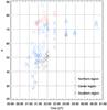 |
Fig. 2 Time-variation of the shear angles θ of the observed post-flare loops, during the development of the flare. θ is the angle between the PIL and the segment that joins the footpoints of the post-flare loops. Different marks are used for different sections of the PIL. |
3. MHD simulation for eruptive flares
3.1. Initial conditions
We simulate the formation of post-flare loops resulting from the so-called “flare reconnection”, which occurs in the vertical current sheet that develops in the wake of a freely erupting twisted coronal flux rope. This is achieved through the calculation of one zero-β time-dependent 3D MHD relaxation, of the continuously-driven simulation of Aulanier et al. (2010).
In the driven simulation, a forward-S sigmoid surrounding a twisted flux rope developed and eventually erupted in an asymmetric initially potential bipolar magnetic field. These settings were driven by observations of typical decaying and erupting ARs (van Driel-Gesztelyi et al. 2003; Green et al. 2011). The quasi-static formation of the rope, starting at the time t = 23 tA, was driven by the sub-Alfvénic shearing line-tied motions combined with simultaneous slow magnetic field diffusion, both applied at a photospheric boundary (in a similar way as in Amari et al. 2003; Mackay & van Ballegooijen 2006). The simulated sigmoid developed asymmetrically, with one elbow being more spread than the other. In the simulation of Aulanier et al. (2010), the rope eventually accelerated upwards from t = 110 tA, and its subsequent fast eruption after t = 120 tA was found to be due to the ideal torus instability (see Bateman 1978; Kliem & Török 2006; Démoulin & Aulanier 2010, for the theory).
For the purpose of this paper, we perform a new simulation of the flux rope eruption. We use the magnetic field at t = 125 tA, and we reset the time to zero. Thus, we consider an initial magnetic field, which is in a clearly torus-unstable regime. We set the plasma density to its initial distribution at t = 0 tA. This allows to start with a relatively smooth density distribution. Finally, we reset the velocities to zero. In this way we get rid of the flows caused by the pre-eruptive driving, so that the rope solely evolves in response to its initial internal Lorentz forces.
Since the May 9, 2011 flare studied in Sect. 2 took place in the decaying remnant of an AR, and since it also involved an asymmetric sigmoid, the present MHD relaxation from a “flux cancellation” asymmetric simulation is particularly well suited for comparison with the observations. The main difference is that the observations display a reversed S-shape sigmoid, whereas the model incorporates a forward-S structure. Either can be made to match the other by a simple mirroring of the images, which only corresponds to a change in sign of the magnetic helicity in the corona.
3.2. Equations and numerical domain
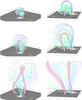 |
Fig. 3 Three-dimensional plots of the time-evolution of selected magnetic field lines. The left column is a projection view which shows the CME in most of the numerical domain. The right column is a zoom on the central and lower regions, which shows the post-flare loop formation at a viewing angle along the PIL. The greyscale images show the vertical component of the photospheric magnetic field Bz(z = 0). |
The simulation is performed with the Observationally-driven High-order scheme Magnetohydrodynamic code (OHM: Aulanier et al. 2005). In its zero-β version, the code advances in time the primitive variables ρ (the mass density), u (the fluid velocity) and B (the magnetic field), by solving the following equations in Cartesian coordinates: 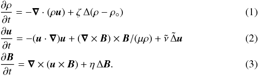 The equations are implemented in their fully developed form, in which all the ∇·B terms are omitted. Neither the electric field nor the current density are calculated in the equations, but the latter is calculated as
  for analyzing.
η ΔB is a collisional resistive term, which is responsible for magnetic reconnection in the simulations. The resistivity η is a constant in the domain, except in the photospheric plane at z = 0 where it is set to zero. ζ and  are other constant diffusion coefficients, further described in Sect. 3.3.
The present simulation is done in the same domain x;y ∈ [ − 10, 10] and z ∈ [0, 30] , and uses the same non-uniform mesh nx × ny × nz = 251 × 251 × 231 points as in Aulanier et al. (2010). The mesh intervals range from 0.006 at x = y = z = 0, and reach maximum values of 0.6 (resp. 0.32) at large z (resp. | x | and | y | ). The z direction is the altitude and z = 0 is the photospheric plane. The calculations are performed in non-dimensionalized units, using μ = 1. The velocities are normalized to the averaged Alfvén speed  , and the time unit tA = 1 is defined as the travel time over a distance d = 1 at the velocity
  .
.
3.3. Boundary conditions and diffusion coefficients
The boundary conditions are open at all faces of the domain, except at z = 0 where line-tied conditions are prescribed.
For the simulation presented in this paper, a damping term was also applied to the Lorentz force over a few mesh points for z > 0 during the full simulation, and over a few mesh points for y ≥ −10 for t ∈ [0, 16 tA] . Both layers were needed to stabilize numerical instabilities arising from a few places where barely resolved current sheets had developed during the continuously driven simulation. These instabilities were not a problem in the driven simulation, presumably because the waves resulting from the driven shearing motions greatly reduced the rate of collapse of these current sheets.
Due to the weakly diffusive high-order scheme of the OHM code, and because of the highly non-uniform mesh, explicit non-physical diffusive terms are needed to smooth sharp density and velocity gradients. ζ Δ(ρ − ρ°) applies to the density. Its form conserves mass, and it ensures that only the density perturbations that develop against the initial density ρ° = ρ(t = 0) can diffuse.  applies to the velocity.
  is a pseudo-Laplacian that applies to mesh units rather than to spatial units.
Physically, the velocity filter would lead to a viscous term νvarΔu, in which νvar would be a space-varying kinematic viscosity. This setting allows to calculate νvar = ν (L/l)2, where L is the size of the largest interval among the three directions of the local mesh, l is the size of the smallest mesh interval within the computational domain (here l = 0.006), and  is the kinematic viscosity effective at the smallest mesh interval. Numerically speaking, this viscous filter leads to a viscous time-scale at the scale of every local mesh interval,
  =
=  , which is constant in the full domain. Thus, the viscous effects are equally effective everywhere in the domain, regardless of the non-uniformity of the mesh. This is particularly well adapted to the present simulation, where large velocities develop where the non-uniform mesh is the most stretched.
Since the diffusion coefficients (η, ζ and ν) are constant in space, and since the numerical scheme is very weakly diffusive, the diffusion can be strictly controlled during the simulation. Comparing with the use of artificial or hyper diffusion schemes, the advantage of this control is that the physical regime of the simulations is known and quantifiable at all times. But one disadvantage is that the diffusion coefficients are neither necessarily optimum at a given time, nor always sufficient to prevent gradients from developing at the scale of the mesh, which can lead to quickly-growing numerical instabilities. Hence we performed several simulations, using various combinations for the values of the diffusion coefficients, and allowing them to be modified a few times throughout the evolution of the system. The simulation on which this paper is based is the best suited, in terms of ensuring the least possible diffusive behavior during the longest time-intervals, and using a minimum number of resettings for the diffusion coefficients. Their values are given in Table 1. For all time-intevals, the magnetic Reynolds number of the eruption is of the order of Rm ~ 1/η.
With these settings, the system smoothly evolves up to t = 46 tA. After this time, the thickness of the flare current sheet (described hereafter in Sect. 4.1) reaches the scale of the mesh. This collapse is mostly caused by the magnetic pressure force in the current sheet itself. Since the calculations are performed in the zero-β regime, there is no thermal pressure force that can counteract this typical current-sheet collapse, and thus numerical instabilities eventually halt the simulation. Of course, the latter could be prevented by re-increasing the diffusion coefficients. But for the purpose of the present study, we did not do as such, because we conservatively considered that doubling the resistivity η one more time would result in a too low Rm.
4. The simulated eruption
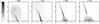 |
Fig. 4 Two-dimensional rendering of the electric currents that develop in the wake of the CME, along a vertical cut at y = −0.3. The CME is visible in the first two panels. All panels show the gradual formation of an inverse Y-shaped current pattern, which results from the flare reconnection in the vertical current sheet. |
4.1. The CME and the flare
As previously reported in Aulanier et al. (2010), the MHD relaxation of the flux rope leads to its free expansion, thus producing a CME. In the following, we use the Topology and field line Tracing code (TOPOTR: Démoulin et al. 1996) to analyze the simulation results.
The evolution of well-chosen representative CME-related magnetic field lines is drawn in Fig. 3. These field lines were chosen so as to show smooth magnetic surfaces. Random field line plotting would show, however, complex and interleaved flux tubes.
The yellow field line is as close as we could find to the axis of the pre-eruptive flux rope. The red/pink lines show the innermost part of the pre-eruptive flux rope, where the twist is concentrated and peaks to 2π. The cyan/green field lines are sheared loops which overlay the flux rope, and the dark blue field lines are very weakly sheared, nearly potential, outer arcades. The relatively weak and concentrated twist in pre-eruptive field a-priori makes it hard to distinguish from a mere sheared arcade (as modeled e.g. in DeVore & Antiochos 2000; Aulanier et al. 2002), but a topological analysis clearly shows that the pre-eruptive field comprises a twisted flux rope (see Savcheva et al. 2012). We will show in Sect. 5.4 that the spatial distribution of magnetic shear in the pre-eruptive magnetic field is the primary cause of the formation of sheared post-flare loops.
Values for the diffusion coefficients.
The right column of Fig. 3 displays a projection-view that is almost aligned with the y axis of the domain, which is nearly aligned with the axis of the pre-eruptive (red/cyan) flux rope. Its upward eruption occurs co-temporarily with a sequence of magnetic reconnections, between weakly sheared (cyan/green) arcades. These reconnections result in forming a twisted (cyan/green) envelope around the inner flux rope, and a growing set of (cyan/green) post-flare loops in the wake of the CME.
Figure 4 provides a two-dimensional analysis of the electric currents which form in a vertical (x,z) cut close to the center of the domain (y = −0.3). It shows that a relatively wide vertical current layer is already present at t = 0, joining a higher-altitude hollow-core current structure surrounding the inner pre-eruptive flux rope. Aulanier et al. (2010) and Savcheva et al. (2012) reported that this current layer had gradually formed around a hyperbolic flux tube, during the energy build-up phase of the flux rope. Figure 4 shows the evolution of three types of current features. Firstly, the narrow current layer stretches vertically in the wake of the CME. As it gets thinner and thinner in time, it can be considered to turn into a current sheet. Secondly, the magnitude of the extended currents on both sides of the current sheet decreases. Thirdly, an inverse Y-shaped current layer grows beneath it, in both vertical and horizontal directions. This growing cusp is the standard signature of the flare reconnection, and it is related with the formation of the (cyan/green) post-flare loops plotted in Fig. 3.
The right column of Figs. 3 and 4 show that the 3D simulation is consistent with the 2D standard model (see Sect. 1).
Magnetic and kinetic energies, and time-scale of the simulated eruption, given in numerical and physical units.
4.2. Expanding and leaning field lines
The left column of Fig. 3 displays a projection-view that allows to see three-dimensional effects. At first sight, this view shows that all the field lines expand vertically during the eruption, and that the axis of top of the (red/pink) twisted flux rope develops a writhe in the late stages of the eruption. Both are consistent with other 3D CME simulations calculated with different MHD codes (Amari et al. 2003; Török et al. 2010, Figs. 11 from both papers), as well as with recent multi-wavelength observations of erupting flux ropes and coronal arcades (Zhang et al. 2012).
In addition, Fig. 3 shows that the outer envelope of sheared loops, which overlay the flux rope all over its length, form a bubble that expand in all directions during the whole simulation. This expansion also occurs along the y axis, which is not treated in 2D models. The sideways leaning of field lines, at the edge of the expanding CME bubble, was already noted by Schrijver et al. (2008, Fig. 9). It is similar to what is seen in several off-limb coronal observations of CMEs, as shown e.g. in the online movies of Warren et al. (2011, Fig. 3) and Schrijver et al. (2011, Fig. 16).
In our simulation, the bubble is not axisymmetric: it expands more along y than along x. These relative extensions are due to different horizontal magnetic pressure forces, which are stronger perpendicularly to the rope axis (i.e. along x): the presence of line-tied loops with vertically-oriented legs along x leads to a stronger confinement. This is the reason why horizontal cross-sections of this bubble in (x,y) planes as plotted in Schrijver et al. (2011, Fig. 20) display an oval shape.
4.3. Inner vertical straightening
A careful look at Fig. 3 can reveal another three-dimensional effect in the evolution of the low altitude sections of the expanding overlaying sheared field lines (in cyan/green) during the flux rope expansion.
The inner legs of these sheared field lines (being rooted at low |x| and |y|, close to the PIL) tend to become more and more two-dimensional, i.e. their extension along the y-direction diminishes. This vertical staightening is opposite to the evolution of the outer legs of the same field lines (being rooted at larger |y|), which lean sidewards as noted above.
To the author’s knowledge, this field line behavior has never been explicitly mentioned before in three-dimensional simulations of free eruptions. Nevertheless, it can be related to the long-term diminishing of the shear-component of the field in 2.5D models for the quasi-static expansion of line-tied shearing bipolar fields (Amari et al. 1996, Sect. 2.2.1.b). In our simulation, it is associated with the decrease of the extended currents on both sides of the current sheet (see Sect 4.1). We argue that this effect is present in most 3D CME models.
This straightening is better shown and quantified in Sect. 5.5. There, we will explain how it plays an important role in the formation of less-and-less sheared post-flare loops.
4.4. Energetics and time-scales
During the time δt = 46 tA of the simulation, the magnetic field energy decreases by δEB and the kinetic energy increases to δEk = Ek(t = 46). The energies are reported in Table 2 in percentage of the initial magnetic energy EB(t = 0). They are also reported in the non-dimensionalized units of the simulation, along with the peak magnetic field Bmax and the horizontal size dAR of the magnetic bipole in the photosphere (at z = 0), as well as with the average Alfvén speed in the corona. The values are also given in physical dimensions, choosing realistic normalizations within the observed ranges, for typical young/compact and for decaying/extended ARs (see e.g. van Driel-Gesztelyi et al. 2003; Régnier et al. 2008).
Table 2 shows that δEB/δEk ~ 21. This ratio is consistent with the values found in other 3D MHD simulations of CME triggering (see e.g. Amari et al. 2003; Lynch et al. 2008). Nevertheless, it is worth noticing that 2.5D simulations typically lead to smaller δEB/δEk ~ 3 (see e.g. Linker et al. 2003; Jacobs et al. 2006; Reeves et al. 2010). In the present simulation, the magnetic energy release is due to four effects: first, the ideal decrease of the magnetic energy density in the CME which expands in all three directions; second, the resistive diffusion of the magnetic fields which are brought into the flare current sheet; third, the weak (but extended) resistive diffusion of the whole system; fourth the viscosity in the simulation tends to diffuse the velocities and therefore diminishes the inertia. The third and the fourth effects are numerical, and they are unavoidable in non-ideal MHD simulations. But the second effect is physical, being related to magnetic reconnection.
In the simulation, the reconnection-related magnetic energy decrease can neither be converted into heat nor into particle acceleration in our zero-β MHD simulation. But both are important in solar flares. It is then arguable that, in the model, the flare reconnection dominates the magnetic energy release, so that the total flare (resp. the CME) energy can approximatively be given by δEB − δEk, (resp. by δEk).
 |
Fig. 5 Three-dimensional plots of selected reconnecting field line pairs, chosen at three different times throughout the simulation (at t = 15,30,45 tA). In the upper (resp. lower) panels, the field lines are drawn before (resp. after) their reconnection. The small blue circles indicate the fixed footpoints at z = 0, from which each green/red field line pairs are integrated, both before and after they reconnect. The inserts on the right show the same cropped field lines as drawn in the third column, but plotted with their full lengths. The thin red/pink flux rope is the same as plotted in Fig. 3. The greyscale images (resp. the overplotted contours) show the vertical component of the electric current |

Let us discuss the physically dimensionalized values from Table 2. On the one hand, the modeled energy values are typical of those estimated in solar flares (Emslie et al. 2005; Fletcher et al. 2011) and CMEs (Vourlidas et al. 2000, 2010). On the other hand, they are contradictory with the findings of Kretzschmar (2011) who estimated lower flare energies, and with those of Emslie et al. (2005) who estimated that both the flare and the CME should have comparable energies. These discrepencies may be related to the efficiency of magnetic energy conversion into flare emissions, during magnetic reconnection. While this aspect is not treated in our zero-β simulation, Reeves & Forbes (2005) have indeed shown that all things being equal, the faster the reconnection takes place, the smaller the fraction of magnetic energy is converted into thermal energy, hence into flare emissions. The associated time-scales for the flare readily fit those measured for weakly and highly energetic flares (Sect. 2.3). We thus find that the factor 35 between the May 9, 2011 event and the one studied by Su et al. (2006) may simply be explained by different scalings, for the size and the magnetic field values in the source regions.
These simple scalings also imply that if the same simulated flare would originate from a decaying/extended AR, its mean power would be of the order of  W, while it would be
  W for a young/compact AR. The ratio between both magnetic powers is more than two orders of magnitude. Under the assumption that the same ratio holds for SXR emissions (which is not trivial since it depends on the reconnection rate, see Reeves & Forbes 2005), our scalings are consistent with relatively older (resp. younger) ARs producing C-class (resp. X-class) flares, typically.
5. Origin and evolution of shear in simulated post-flare loops
5.1. J- and Ω-shaped progenitors of post-flare loops
The reconnection-driven formation of many post-flare loops on top of one another is visible in Fig. 3, and is suggested in Fig. 4. Individual pairs of pre-reconnecting (hereafter, progenitor) field lines, each of them forming a post-flare loop as well as a twisted field line in the outer envelope of the CME, are plotted in Fig. 5.
Early in the flare (at t = 15 tA in Fig. 5) the progenitor field lines have a forward J-shape. Their apexes are strongly inclined towards the photosphere, and do not reach the maximum altitude of the flux rope. Thus, the three-dimensional geometry of the early flare reconnection fits the cartoon of the so-called tether-cutting model by Moore et al. (2001). It is worth noticing that this reconnection was already occuring in the driven simulation, several tens of tA before the CME launch (Aulanier et al. 2010). Therefore in our simulation, the early flare reconnection alone does not trigger the CME, unlike in the tether-cutting model. As the flare evolves (at t = 30 tA in Fig. 5) the progenitor field lines are less and less inclined. Still, their apexes remain relatively low-lying when compared to the erupting flux rope.
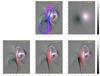 |
Fig. 6 Pre-eruptive magnetic field configuration, evolving post-flare loops and moving photospheric currents, as viewed from above. Upper-right panel: cyan/pink contours and greyscale image of negative/positive magnetic fields Bz(z = 0), with the color scale on the right. The yellow line is the PIL. This magnetic field is fixed in time, so the same contours are reproduced in all panels. Upper-left panel: the pre-eruptive magnetic field configuration. The blue (resp. green) lines are typical sigmoidal and highly sheared (resp. large-scale and nearly potential) arcades. The pink lines show the dipped portions of every concave-up field lines. The greyscale image shows the negative/positive photospheric currents |
In the late phase of the flare reconnection (at t = 45 tA in Fig. 5), the progenitor field lines are nearly two-dimensional. Both field lines that are about to reconnect with one another are Ω-shaped. They are rooted very close to each other in the photosphere, but they diverge from one another at large altitudes, where their apexes pass above that of the flux rope. In an asymptotic two-dimensional geometry (which is never fully reached in the simulation), both field lines would be merged as one, hence this single field line would reconnect with itself and form a detached plasmoid, as in 2D models referred to in Sect. 1.
In spite of the projection views in Fig. 5 which are not best suited to measure magnetic shear above the PIL, one can already see there that the post-flare loop at t = 16 tA is more sheared than the one at t = 31 tA, and also that the one drawn at t = 46 tA is nearly potential. This is better seen in Fig. 6.
5.2. Comparing modeled and observed features
At every time during the simulation, there is a clear relation between the electric currents in the corona (for z > 0) and the boundary layer between pre- and post-reconnected field lines (see Figs. 3 and 4). We analyze their shape and time-evolution in the photosphere (i.e. the line-tied boundary at z = 0) in Fig. 6.
Let us first consider the modeled field lines. In the pre-eruptive field at t = 0, J- and S-shaped sigmoidal field lines are plotted in blue. They were integrated from photospheric footpoints being randomly placed at various distances around those of the flux rope axis (drawn in yellow in Fig. 3). As mentioned in Sect. 4.1, this random choice leads to an interleaved set of field lines. In addition, the dipped portions of every concave-up field lines (i.e. magnetic dips) are plotted as thick pink lines, following the procedure described in Aulanier & Démoulin (1998) and Aulanier & Schmieder (2002). This underlines that a weakly S-shaped solar filament, with a small interruption in its center, can exist in the pre-eruptive configuration. During the flare development for t ≥ 15 tA, post-flare loops are drawn as sets of red field lines. For each set, all the field lines reconnected between 1 tA and 2 tA before the time of each panel, in the same way as shown in Fig. 5. The strong-to-weak shear variation in these post-flare loops is qualitatively clearer than in Fig. 5. It is quantified hereafter in Sect. 5.3.
The field line plots show that the modeled asymmetric sigmoid (drawn in blue in Fig. 6), filament (drawn in pink), and post-flare loops (drawn in red) are similar to the observed ones (see Fig. 1), albeit for the mirroring which has to be applied, either to the model or to the observations, to get the same sign for the magnetic helicity (see Sect. 3.1).
Let us now focus on the photospheric electric currents plotted in Fig. 6. At all times during the simulation, they display three distinct patterns within each of the two magnetic flux concentrations: around the center of the polarity, several patches of extended currents of both signs, with stronger so-called direct-currents ( , for our simulated forward J-shaped sigmoidal blue field lines) and weaker return-currents (α < 0); at the outer edge of the polarity, an arc-shaped narrow current layer, which also involves direct- and return-currents; parallel and close to the PIL, a long and narrow current layer, with direct-currents only. Hereafter the latter will be referred to as a “current-ribbon”. Both current-ribbons are nearly parallel to each other, on both sides of the PIL. Each of these photospheric currents have different time-evolutions and relations with coronal field lines. The arc-shaped currents almost do not evolve. Depending on the location, they weakly move either towards or away from the center of the magnetic flux concentrations. The extended currents almost stay in place, but their magnitudes diminish in time. This is related to the decrease of the twist per unit-length of the expanding inner flux rope, since its length increases while its end-to-end twist remains constant. This is a natural property of line-tied coronal fields modeled in the MHD paradigm (as explained in Aulanier et al. 2005, Sect. 6.2). This current decrease is not present, however, in circuit-models of solar flares, since the latter fix the currents at the photospheric boundary (Melrose 1995). Nevertheless, it is present in electric-wire flare models, which incorporate MHD properties (Démoulin & Aulanier 2010). Early in the flare, both current-ribbons are offset from one another with respect to the center of the magnetic bipole. During the flare, they weakly extend in length along the y-axis, thus their relative offset diminishes. Also, both current-ribbons move away from the PIL in the x-direction, towards the centers of the magnetic polarities.
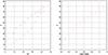 |
Fig. 7 Left: time-evolution of the shear angle θ of the post-flare loops which pass above the center of the PIL at x = y = 0. The 10 blue plus signs stand for the post-flare loops that have reconnected at most 1 tA before the times at which they are drawn. Their corresponding loop apexes are z = 0.2,0.3,...,1,1.1. The red diamonds correspond to the post-flare loops passing through the same z values, which have formed at later times during the flare, while the former loops have relaxed and shrunk to lower z values. Right: dispersion of θ values of the post-flare loops along the PIL at t = 46 tA, as a function of the altitude z of their apex. In both panels, θ values are measured from the footpoints of the post-flare loops. |
Finally, we can relate field lines to photospheric currents. Whichever time is considered, Fig. 6 shows that the recently formed postflare loops are always rooted at the inner edge of the current-ribbons, i.e. on the side which is the closest to the PIL. Also, their positions in x, as measured at y = −0.3 in Fig. 6, exactly fit those of the footpoints of the inverted Y-shaped coronal cusp plotted in Fig. 4. Thus both are the same structure. So, referring to the standard CSHKP in 2D, we conjecture that the simulated photospheric current-ribbons should correspond to flare ribbons. By continuity, we argue that each of the arc-shaped photospheric currents could be associated with the hook that is located at the extremity of each flare ribbon. This is also supported by the fact that, both in the model and in the observations, these structures surround the footpoints of the pre-eruptive sigmoid (compare Figs. 1 and 6, mirroring one of them).
All these results show that our three-dimensional extensions of the standard flare model suggest that bright J-shaped flare ribbons (as observed in multi-wavelength imagery) which are offset from one another along the PIL, and which move apart from each other perpendicular to the PIL, should be closely matched by J-shaped concentrations of vertical electric currents (as calculated from vector magnetograms).
5.3. Quantifying the strong-to-weak shear transition
Similarly to the observational analysis (see Sect. 2.3), we quantify the strong-to-weak shear transition in each modeled post-flare loop by measuring the angle between the segment that joins the field line footpoints with the orientation of the PIL. The origins of this transition are discussed in Sects. 5.4 and 5.5.
The same reference is chosen, i.e. θ = 90° (resp. 0) stands for post-flare loops being orthogonal to (resp. aligned with) the PIL. A slight difference with the observational analysis is that we now consider the local orientation of the PIL underneath the crossing point with this segment, since this information is readily available in the model. The time-evolution of the shear angle θ of each newly reconnected post-flare loop whose apexes are located at x = y = 0 is plotted with plus signs in the left-panel of Fig. 7.
Note that at the times when θ is measured, these field lines have not yet reached a force-free state. Indeed, the downward magnetic tension of newly reconnected field lines and the underlying magnetic pressure of previously reconnected ones do not balance right away. In the simulation, it takes more than 10 tA for the field lines to relax magnetically towards a force-free equilibrium. On the one hand, it is not clear at what time post-flare loops are typically observed in EUV at 195 Å during this relaxation. But on the other hand as mentioned in Sect. 2.3, the θ values measured with field lines footpoints remain constant during this magnetic relaxation under the line-tying assumption. Thus, the θ values given by the plus signs can be compared to the observed ones reported in Fig. 2. To be conservative, we also measure the shear angle distributions for the post-flare loops present at t = 46 tA. The diamond signs in the left panel of Fig. 7 stand for the θ values for the post-flare loops which are all present at the same time t = 46 tA, at the same altitudes and positions above the PIL as the newly reconnected ones. The right panel of Fig. 7 displays the spatial variations of θ with height z. The bars there indicate how much θ is dispersed along the PIL for each altitude plotted. Within each bar, the largest θ values typically correspond to the central part of the PIL.
There are two similarities between the strong-to-weak shear transitions as measured observationally in Fig. 2 and theoretically in Fig. 7. Firstly, both start with finite shears, i.e. the first post-flare loops are not fully aligned with the PIL. This can be interpreted with the model. Its pre-eruptive magnetic field at t = 0 already incorporated small loops underlying the flux rope. In the driven simulation which brought the system up to this reinitialized t = 0, these loops had already formed by means of a tether-cutting reconnection type, thus contributing in the flux rope formation and rise in altitude up to its eruptive threshold (Aulanier et al. 2010). The vertical current layer displayed at t = 0 in Fig. 4 is indeed broader at low altitudes. This corresponds to a cusp-shaped current pattern at low altitude, albeit a small-scale one (see the topological analysis reported in Savcheva et al. 2012, for the pre-eruptive configuration). Secondly, both the observations and the model do not reach a potential state with post-flare loops being orthogonal with the PIL (i.e. with θ = 90°). In the model this is due, at least, to a limited calculation time (the reasons of which are discussed in Sect. 3.3).
There are also two differences between the observations and the model. Firstly, the model starts at stronger shears (θ ~ 17°) than the observations (θ ~ 30°). This may be due to intrinsic differences between the idealized modeled magnetic field and the real one. This may also simply be due to the lack of visibility of the very first post-flare loops in the observations. Secondly, the strong-to-weak shear is linear in time in the model, while is reaches an asymptotical state in the observations. Again, this is probably due to the limited time duration of the simulation. On the one hand, it is possible to estimate that the simulation typically lasts for one hour, when using the typical scalings from Table 2. When doing so, the scaled model and the observations can be regarded as being consistent during the first hour of the observed flare. But on the other hand, one should bear in mind that this interpretation is subject to uncertainties: during this first hour of the observed flare, the large dispersion in the θ values makes it difficult to establish a clean curve for θ(t); also the model scalings depend on the precise value of the coronal Alfvén speed, which is not known in the observations.
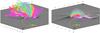 |
Fig. 8 Three-dimensional view of field lines before and after they have reconnected. Right: distribution along the PIL of post-flare loops at t = 45 tA. Each field line is color-coded accordingly with the altitude z = 0.1,0.2,...,1,1.1 of its apex. Left: progenitor field lines at t = 0, plotted from the same footpoints at z = 0 of same the post flare loops as drawn in the right panel. In both panels, a differential shear is present, with a shear decreasing away from the PIL. |
5.4. Shear transfer from pre- to post-eruptive field
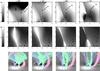 |
Fig. 9 Upper and middle panels: two-dimensional rendering of the shear angle θ and the inclination angle ψ along a vertical cut at y = −0.3. θ and ψ values are there measured from the local magnetic field components. The full (resp. dashed) contours correspond to negative (resp. positive) values and are labeled in degrees. Lower panels: three-dimensional zoom of the same field lines as drawn in Fig. 3, showing the time-evolution of their vertical straightening around the PIL. These panels all together show a gradual decrease of shear and inclination for the low-altitude magnetic fields, before they reconnect. |
As shown in θ plots from Fig. 7, the strong-to-weak shear transition in time also results in a strong-to-weak shear spatial distribution for post-flare loops around the PIL. So the flare results in the formation of a differential magnetic field in the active region (Schmieder et al. 1996). Since the vertical magnetic field is fixed at the line-tied boundary, the late distribution of shear cannot be caused by the emergence of a new twisted flux tube (as proposed by Asai et al. 2003). Also, it is related to a clear diminishing shear in the post-flare loops rooted farther and farther away from the PIL (oppositely to the findings of Inoue et al. 2011). In our model, the late differential magnetic shear at t = 46 tA rather reflects the early one at t = 0. This can be shown with two independent analyses.
Firstly, it is qualitatively obvious in Fig. 8. There, initial progenitor field lines and final post-flare loops are plotted, with all field lines being integrated from the same photospheric footpoints at z = 0 at both times.
It can be seen that each lowermost and shearedmost post-flare loop (at t = 45 tA, drawn in pink and fuchsia in the left panel) has been formed by reconnection of a pair of the most sheared and inclined J-shaped progenitor field lines rooted close to the PIL (at t = 0, drawn in the same colors in the right panel). By continuity, each of the highest and least sheared post-flare loop (drawn in blue and black) comes from nearly potential and vertical Ω-shaped progenitor field lines rooted far from the PIL. These results for a wide set of field lines are consistent with our early findings from Fig. 5, which only addressed three individual post-flare loops.
Secondly, it can be quantitatively measured by comparing the spatial distributions of the local shear angle θ, at the start and the end of the simulation. The knowledge of the coronal magnetic field in the simulation indeed allows to calculate θ at all times, as being defined by ratios between magnetic field components instead of by field line footpoints, as done before. This angle is calculated as: 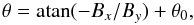 (4)where θ0 is the angle made by the PIL and the y axis at y = y0. For simplicity, we measure θ in the same 2D cut as in Fig. 4, i.e. at y = y0 = −0.3. It is plotted in the first row of Fig. 9. This definition leads to the following properties: | θ | = 90° refers to an unsheared field with By = 0 (i.e. the field is purely contained in the plane of the cut); θ = 0 either refers to an infinitely sheared field (i.e. the field is aligned with the PIL), or to a region where the Bx component changes sign (i.e. the field projected in the plane of the cut is vertical); since By < 0 dominates in the field-of-view of Fig. 9 (i.e. the By component points out of – not into – the plane of the cut), then θ < 0 (resp. > 0) values being drawn in dark (resp. light) colors in Fig. 9 mostly correspond to areas where Bx < 0 (resp. > 0), i.e. where the field projected in the plane of the cut points to the left (resp. to the right), which is the normal (resp. inverse) polarity of the photospheric bipole. In the few regions where By > 0, we add or subtract 180° depending on the sign of Bx, so as to finally obtain θ ∈ [−180°,180°] . With a simple change in sign, this definition for θ permits to be consistent with the footpoint-related θ measurements plotted in Figs. 2 and 7.
Comparing Figs. 4 and 9 at t = 0, one can see that the shearedmost regions (i.e. where | θ | < 10°) are located at all heights around the current sheet and the flux rope. Initially (at t = 0), and at low heights near the footpoints of the progenitor field lines (which eventually turn into the first post-flare loops), | θ | increases up to 20° (i.e. the shear decreases) away from the PIL along x. At later times (see t = 45 tA), and at the same low heights, the distribution of θ displays a quasi-linear decrease of shear with z above the PIL, as well as a decrease of shear away from the PIL along x. Qualitatively, the former is in agreement with footpoint-related shear angle measurements (see the right-panel of Fig. 7). The latter is also consistent with a reconnection-driven transfer of magnetic shear from the pre-eruptive field at t = 0 to the post-eruptive field (see also Figs. 6 and 8).
These two independent proxies reveal that, qualitatively speaking, the differential magnetic shear in post-flare loops reflects that of the pre-eruptive fields. Indeed, the latter incorporate a sheared sigmoidal core, and an outer weakly sheared envelope. This confirms the interpretation by Su et al. (2006, Fig. 11).
Nevertheless, Fig. 9 highlights that this process, alone, cannot quantitatively account for the late differential shear. Indeed during the flare, the distribution of θ gradually forms a cusp in 2D, which is broader than that of the electric currents (compare with Fig. 4). While this broad cusp grows in size, its edges become darker and darker (i.e. the | θ | increases). This means that the magnetic shear in the progenitor field lines decreases in time, from their initial state at t = 0 up to the time at which they reconnect in the current sheet. This shows that another physical effect than the shear transfer from the pre- to the post-eruptive magnetic field should be at work in the coronal magnetic field, in the strong-to-weak shear transition in post-flare loops. This effect is identified hereafter.
5.5. Vertical straightening of progenitor field lines
The evolution of magnetic shear in pre-reconnecting progenitor field lines can be estimated not only from the local shear angle (see Eq. (4)), but also from the local inclination angle of the field. This angle is calculated as: 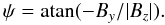 (5)Note that ψ does not measure the full inclination of the magnetic field, since it does not incorporate the Bx component. ψ rather measures the inclination of the magnetic field with respect to the y-axis only. It is plotted in the middle row in Fig. 9. With this definition, and since By < 0 in the region drawn in Fig. 9, then ψ ∈ [0°,90°] . Also, ψ = 90° refers to magnetic fields which are purely horizontal (i.e. where Bz = 0). Finally, ψ = 0 corresponds to magnetic fields being orthogonal to the PIL (i.e. vertical where Bx = 0). In summary, smaller (resp. larger) ψ values as plotted in dark (resp. light) colors in Fig. 9 typically show regions where the magnetic field tends to be more (resp. less) vertical with respect to the y axis.
During the eruption, Fig. 9 shows that the larger ψ regions get more and more concentrated in and around the vertical current sheet. At large heights, this may be attributed to the motions of the large-scale field lines towards the current sheet. But at lower heights around the cusp of the electric currents, the decrease of ψ cannot be related to these converging motions. It rather corresponds to a CME-related vertical straightening of lower sections of pre-reconnecting field lines rooted in the vicinity of the PIL. This geometrical evolution was already briefly noted in Sect. 4.3. The lower panels of Fig. 9 show zoomed-in portions of the same field lines, with the same projection view, as in Fig. 3. There, the vertical straightening of the lower sections of the cyan and green large-scale field lines, before they reconnect and form small-scale post-flare loops, is more clearly seen that in larger fields-of-view.
In terms of MHD equations, this anisotropic expansion from the line-tied photosphere (where u(z = 0) = 0) leads to ∇·u > 0, with ∂uz/∂z > 0 being dominant. Since By < 0 in this region, the − By∂uz/∂z term on the right hand-side of the y component of Eq. (3) is positive. When one neglects the other ideal terms which are related to the relatively weaker horizontal velocities, this leads to ∂By/∂t > 0. This naturally accounts for an increase of the negative By values, thus for a decrease of | By | , and therefore for the measured decrease of the ψ angle.
The diminishing inclination of progenitor field lines (during the time interval t ∈ [0,treco] ) leads to bring together (within the current sheet at t = treco) pairs of field lines which were initially (at t = 0) not facing one another on both sides of the vertical current sheet, and which were more sheared than at the time at which they reconnect (at t = treco). In the asymptotic case, i.e. for By → 0, this would lead to a purely 2D planar reconnection, in which a single progenitor field line would pinch and reconnect with itself within the current sheet. This would lead to the formation of a truly potential post-flare loop, whatever the pre-eruptive shear of the progenitor field line. In the general case, the resulting effect is to form post-flare loops having less magnetic shear than they would have, if their progenitors would not have straightened before the reconnection.
Finally, the ideal low-altitude vertical straightening of coronal field lines before they reconnect accounts for the quantitative discrepancies identified in Fig. 8, between the pre- and the post-eruptive differential magnetic shears around the PIL. Thus, our analyses imply that the interpretation for the strong-to-weak shear transition in post-flare loops, in terms of shear transfer from the pre- to the post-eruptive magnetic field (see Sect. 5.4 and Su et al. 2006, Fig. 11), must be extended such that an extra-weakening of the shear in outer post-flare loops is also provided by the vertical expansion of the field during the CME.
6. Conclusions
6.1. Summary
To account for several observed properties of solar eruptive flares, the standard CSHKP model needs to be extended in three-dimensions. In this work we addressed part of this problem.
We performed and analyzed a generic non-dimensionalized 3D MHD simulation with the OHM code, of an asymmetric solar eruption. In the simulation, a flare occurs in the wake of a coronal mass ejection (CME), the latter carrying away 5% of the released magnetic energy. Dimensionalizing the model with typical young and decaying solar active region scalings, we found flare energies and time-scales that are consistent with typical observed estimations. The simulation was compared with STEREO and SDO observations of the May 9, 2011 eruptive flare. This event originated from the remnant of an isolated bipolar active region that had a relatively smooth polarity inversion line (PIL). Many morphological consistencies were found between the model and the observations.
We identified several three-dimensional physical processes which could be generic in eruptive solar flares, regarding: the electric currents within photospheric magnetic flux concentrations, from which flares originate; the J-shapes and the offsets of chromospheric flare ribbons, which form and spread on both sides of the PIL during flares; the strong-to-weak shear transition which develops in post-flare loops, either inferred from pairs of ribbon kernels or directly observed for the loops themselves.
6.2. Extensions to the CSHKP model
Our results provide new three-dimensional extensions to the standard flare model. They can be summarized as follows:
-
1.
The broad electric currents being present in the photospherewithin sunspots and faculae incorporate both direct and returncurrents. The former dominate over the latter. The currentdensities decrease in time during the eruption. This is due to thedecrease of twist per unit-length within the expanding line-tiedCME flux tube.
-
2.
The J-shape pattern seen in emission in each flare ribbon corresponds to a narrow electric current layer. The straight part of the J, which is parallel to the PIL, involves direct currents only. This part corresponds to the footpoints of the cusp which forms below the vertical current sheet, within which the flare magnetic reconnection develops in the wake of the CME. The curved hook of the J involves both direct and return currents. This part surrounds the legs of the expanding CME flux tube.
-
3.
The strong-to-weak shear transition which develops in time, in the post-flare loops, eventually results in a differential magnetic shear in space, within the post-eruptive coronal field. The resulting magnetic shear decreases away from the PIL. The initial offset of flare ribbons from one another corresponds to the magnetic shear in the early-formed post-flare loops.
-
4.
The post-eruptive differential magnetic shear qualitatively reflects that of the pre-eruptive sheared loops which overlay filaments and sigmoids, and which are themselves surrounded by large-scale nearly-potential arcades. Thus, the strong-to-weak shear transition is partly due to the reconnection-driven shear transfer from the pre- to the post-eruptive magnetic field. But an over-weakening of the shear occurs in the outer post-flare loops. So the shear transfer alone cannot account for the strong-to-weak transition quantitatively.
-
5.
During the eruption, the inner legs of the sheared field lines which surround the erupting flux tube, and which eventually reconnect and form post-flare loops, straighten vertically as viewed perpendicularly to the PIL. This is due to the magnetic field expansion in the legs of the CME at low altitudes, which is faster vertically than horizontally. These changes in inclination eventually allow magnetic reconnection between pairs of loops that are different than those which would have interacted with one another in a non-erupting field, and whose photospheric footpoints are less offset from one another along the PIL. The resulting post-flare loops, being rooted in these less offset footpoints, are thus not as sheared as they would have been in a non-eruptive flare. Asymptotically, this vertical stretching would result in potential post-flare loops, regardless of the initial shear in their pre-eruptive progenitor loops.
6.3. Discussion
Even though the setup for the specific simulation performed in this paper was driven by typical solar observations, the physical mechanisms which we identified and which we propose as new extensions to the standard flare model will still have to be tested by independent studies so as to check whether they are generic or not.
On the one hand, the occurence of these mechanisms should be sought in other analytical and numerical models for solar eruptions which also satisfy observational constrains.
On the other hand, our results provide theoretical predictions that should be tested with direct observations. Firstly, the time-evolution and spatial distribution of electric currents in the photosphere, which presumably also exist in the chromosphere, will have to be measured with series of vector magnetograms. The acquisition-time of each magnetogram and the time-interval between each of them will have to be short enough to allow a good sampling to follow the displacement of flare ribbons. Secondly, the vertical straightening of the legs of sheared coronal loops will have to be directly visualized with EUV or soft X-ray imaging telescopes. This observation will presumably require seeing the flare with a favorable projection angle, and using relatively hot channels to visualize the sheared coronal loops, which are often not visible in warm EUV channels. The current SDO and the future Solar Orbiter spacecrafts should be particularly well suited for these purposes.
Other three-dimensional features that were not addressed in this study probably also exist in eruptive flares. Among those are the relation between flare ribbons and topological features of the magnetic field, as well as the slip-running nature of the flare reconnection. These issues will be addressed in the second paper of this series.
Acknowledgments
We acknowledge the use of STEREO and SDO data, and we thank the SECCHI and HMI teams for their open data policy. The MHD calculations were done on the quadri-core bi-Xeon computers of the Cluster of the Division Informatique de l’Observatoire de Paris (DIO). The work of M.J. is funded by a contract from the AXA Research Fund.
References
- Amari, T., Luciani, J. F., Aly, J. J., & Tagger, M. 1996, ApJ, 466, L39 [NASA ADS] [CrossRef] [Google Scholar]
- Amari, T., Luciani, J. F., Aly, J. J., Mikic, Z., & Linker, J. 2003, ApJ, 595, 1231 [NASA ADS] [CrossRef] [EDP Sciences] [Google Scholar]
- Asai, A., Ishii, T. T., Kurokawa, H., Yokoyama, T., & Shimojo, M. 2003, ApJ, 586, 624 [NASA ADS] [CrossRef] [Google Scholar]
- Aulanier, G., & Démoulin, P. 1998, A&A, 329, 1125 [Google Scholar]
- Aulanier, G., & Schmieder, B. 2002, A&A, 386, 1106 [NASA ADS] [CrossRef] [EDP Sciences] [Google Scholar]
- Aulanier, G., DeVore, C. R., & Antiochos, S. K. 2002, ApJ, 567, L97 [NASA ADS] [CrossRef] [Google Scholar]
- Aulanier, G., Démoulin, P., & Grappin, R. 2005, A&A, 430, 1067 [NASA ADS] [CrossRef] [EDP Sciences] [Google Scholar]
- Aulanier, G., Török, T., Démoulin, P., & DeLuca, E. E. 2010, ApJ, 708, 314 [Google Scholar]
- Bateman, G. 1978, MHD Instabilities (MIT Press) [Google Scholar]
- Cargill, P. J., Mariska, J. T., & Antiochos, S. K. 1995, ApJ, 439, 1034 [NASA ADS] [CrossRef] [Google Scholar]
- Carmichael, H. 1964, NASA Special Publ., 50, 451 [Google Scholar]
- Chandra, R., Schmieder, B., Aulanier, G., & Malherbe, J. M. 2009, Sol. Phys., 258, 53 [NASA ADS] [CrossRef] [Google Scholar]
- Chen, P. F., & Shibata, K. 2000, ApJ, 545, 524 [Google Scholar]
- del Zanna, G., Berlicki, A., Schmieder, B., & Mason, H. E. 2006, Sol. Phys., 234, 95 [NASA ADS] [CrossRef] [Google Scholar]
- Démoulin, P., & Aulanier, G. 2010, ApJ, 718, 1388 [NASA ADS] [CrossRef] [Google Scholar]
- Démoulin, P., Henoux, J. C., Priest, E. R., & Mandrini, C. H. 1996a, A&A, 308, 643 [NASA ADS] [Google Scholar]
- Démoulin, P., Priest, E. R., & Lonie, D. P. 1996b, J. Geophys. Res., 101, 7631 [NASA ADS] [CrossRef] [Google Scholar]
- DeVore, C. R., & Antiochos, S. K. 2000, ApJ, 539, 954 [NASA ADS] [CrossRef] [Google Scholar]
- Emslie, A. G., Dennis, B. R., Holman, G. D., & Hudson, H. S. 2005, J. Geophys. Res. (Space Phys.), 110, 11103 [NASA ADS] [CrossRef] [Google Scholar]
- Fletcher, L., & Hudson, H. S. 2002, Sol. Phys., 210, 307 [NASA ADS] [CrossRef] [Google Scholar]
- Fletcher, L., Dennis, B. R., Hudson, H. S., et al. 2011, Space Sci. Rev., 159, 19 [NASA ADS] [CrossRef] [Google Scholar]
- Forbes, T. G., Linker, J. A., Chen, J., et al. 2006, Space Sci. Rev., 123, 251 [NASA ADS] [CrossRef] [Google Scholar]
- Green, L. M., Kliem, B., & Wallace, A. J. 2011, A&A, 526, A2 [NASA ADS] [CrossRef] [EDP Sciences] [Google Scholar]
- Hirayama, T. 1974, Sol. Phys., 34, 323 [NASA ADS] [CrossRef] [Google Scholar]
- Howard, R. A., Moses, J. D., Vourlidas, A., et al. 2008, Space Sci. Rev., 136, 67 [NASA ADS] [CrossRef] [Google Scholar]
- Inoue, S., Kusano, K., Magara, T., Shiota, D., & Yamamoto, T. T. 2011, ApJ, 738, 161 [NASA ADS] [CrossRef] [Google Scholar]
- Jacobs, C., Poedts, S., & van der Holst, B. 2006, A&A, 450, 793 [NASA ADS] [CrossRef] [EDP Sciences] [Google Scholar]
- Kliem, B., & Török, T. 2006, Phys. Rev. Lett., 96, 255002 [NASA ADS] [CrossRef] [PubMed] [Google Scholar]
- Kopp, R. A., & Pneuman, G. W. 1976, Sol. Phys., 50, 85 [NASA ADS] [CrossRef] [Google Scholar]
- Kretzschmar, M. 2011, A&A, 530, A84 [NASA ADS] [CrossRef] [EDP Sciences] [Google Scholar]
- Lin, J., & Forbes, T. G. 2000, J. Geophys. Res., 105, 2375 [NASA ADS] [CrossRef] [Google Scholar]
- Linker, J. A., Mikić, Z., Lionello, R., et al. 2003, Phys. Plasmas, 10, 1971 [NASA ADS] [CrossRef] [Google Scholar]
- Liu, R., Liu, C., Wang, S., Deng, N., & Wang, H. 2010, ApJ, 725, L84 [NASA ADS] [CrossRef] [Google Scholar]
- Lynch, B. J., Antiochos, S. K., DeVore, C. R., Luhmann, J. G., & Zurbuchen, T. H. 2008, ApJ, 683, 1192 [NASA ADS] [CrossRef] [Google Scholar]
- Mackay, D. H., & van Ballegooijen, A. A. 2006, ApJ, 641, 577 [NASA ADS] [CrossRef] [Google Scholar]
- Masson, S., Klein, K.-L., Bütikofer, R., et al. 2009, Sol. Phys., 257, 305 [NASA ADS] [CrossRef] [Google Scholar]
- Melrose, D. B. 1995, ApJ, 451, 391 [NASA ADS] [CrossRef] [Google Scholar]
- Moore, R. L., Sterling, A. C., Hudson, H. S., & Lemen, J. R. 2001, ApJ, 552, 833 [NASA ADS] [CrossRef] [Google Scholar]
- Pevtsov, A. A., Canfield, R. C., & Metcalf, T. R. 1995, ApJ, 440, L109 [NASA ADS] [CrossRef] [Google Scholar]
- Priest, E. R., & Forbes, T. G. 2002, A&A Rev., 10, 313 [Google Scholar]
- Reeves, K. K., & Forbes, T. G. 2005, ApJ, 630, 1133 [NASA ADS] [CrossRef] [Google Scholar]
- Reeves, K. K., Linker, J. A., Mikić, Z., & Forbes, T. G. 2010, ApJ, 721, 1547 [NASA ADS] [CrossRef] [Google Scholar]
- Régnier, S., Priest, E. R., & Hood, A. W. 2008, A&A, 491, 297 [NASA ADS] [CrossRef] [EDP Sciences] [Google Scholar]
- Robbrecht, E., & Berghmans, D. 2004, A&A, 425, 1097 [NASA ADS] [CrossRef] [EDP Sciences] [Google Scholar]
- Savage, S. L., McKenzie, D. E., & Reeves, K. K. 2012, ApJ, 747, L40 [NASA ADS] [CrossRef] [Google Scholar]
- Savcheva, A., Pariat, E., van Ballegooijen, A. A., Aulanier, G., & DeLuca, E. E. 2012, ApJ, in press [Google Scholar]
- Schmieder, B., Forbes, T. G., Malherbe, J. M., & Machado, M. E. 1987, ApJ, 317, 956 [Google Scholar]
- Schmieder, B., Heinzel, P., Wiik, J. E., et al. 1995, Sol. Phys., 156, 337 [NASA ADS] [CrossRef] [Google Scholar]
- Schmieder, B., Démoulin, P., Aulanier, G., & Golub, L. 1996, ApJ, 467, 881 [NASA ADS] [CrossRef] [Google Scholar]
- Schou, J., Scherrer, P. H., Bush, R. I., et al. 2012, Sol. Phys., 275, 229 [Google Scholar]
- Schrijver, C. J., Elmore, C., Kliem, B., Török, T., & Title, A. M. 2008, ApJ, 674, 586 [NASA ADS] [CrossRef] [Google Scholar]
- Schrijver, C. J., Aulanier, G., Title, A. M., Pariat, E., & Delannée, C. 2011, ApJ, 738, 167 [NASA ADS] [CrossRef] [Google Scholar]
- Shibata, K., & Magara, T. 2011, Living Rev. Sol. Phys., 8, 6 [NASA ADS] [Google Scholar]
- Shibata, K., Masuda, S., Shimojo, M., et al. 1995, ApJ, 451, L83 [NASA ADS] [CrossRef] [Google Scholar]
- Shiota, D., Isobe, H., Chen, P. F., et al. 2005, ApJ, 634, 663 [NASA ADS] [CrossRef] [Google Scholar]
- Sturrock, P. A. 1966, Nature, 211, 695 [NASA ADS] [CrossRef] [Google Scholar]
- Su, Y. N., Golub, L., van Ballegooijen, A. A., & Gros, M. 2006, Sol. Phys., 236, 325 [NASA ADS] [CrossRef] [Google Scholar]
- Su, Y., Golub, L., & van Ballegooijen, A. A. 2007, ApJ, 655, 606 [NASA ADS] [CrossRef] [Google Scholar]
- Török, T., Berger, M. A., & Kliem, B. 2010, A&A, 516, A49 [NASA ADS] [CrossRef] [EDP Sciences] [Google Scholar]
- van Driel-Gesztelyi, L., Wiik, J. E., Schmieder, B., et al. 1997, Sol. Phys., 174, 151 [NASA ADS] [CrossRef] [Google Scholar]
- van Driel-Gesztelyi, L., Démoulin, P., Mandrini, C. H., Harra, L., & Klimchuk, J. A. 2003, ApJ, 586, 579 [NASA ADS] [CrossRef] [Google Scholar]
- Vourlidas, A., Subramanian, P., Dere, K. P., & Howard, R. A. 2000, ApJ, 534, 456 [Google Scholar]
- Vourlidas, A., Howard, R. A., Esfandiari, E., et al. 2010, ApJ, 722, 1522 [NASA ADS] [CrossRef] [Google Scholar]
- Wang, S., Liu, C., Liu, R., et al. 2012, ApJ, 745, L17 [NASA ADS] [CrossRef] [Google Scholar]
- Warren, H. P., O’Brien, C. M., & Sheeley, Jr., N. R. 2011, ApJ, 742, 92 [Google Scholar]
- Wuelser, J.-P., Lemen, J. R., Tarbell, T. D., et al. 2004, in SPIE Conf. Ser. 5171, eds. S. Fineschi, & M. A. Gummin, 111 [Google Scholar]
- Zhang, J., Cheng, X., & Ding, M.-D. 2012, Nature Comm., 3 [Google Scholar]
All Tables
Magnetic and kinetic energies, and time-scale of the simulated eruption, given in numerical and physical units.
All Figures
|
Fig. 1 SDO/HMI and STEREO-B/EUVI observations of the May 9, 2011 eruptive flare. Top panels: the pre-flare sigmoid and filament in EUV, and its magnetic environment three weeks before and one week after the flare. Bottom panels: formation of double J-shaped ribbons and strong-to-weak shear transition in the post-flare loops. The field-of-view is indicated by the white dashed rectangle in the top panel. The yellow line indicates the average orientation of the PIL and the colored marks indicate examples of loop footpoints, both being used to estimate the shear angles. |
| In the text | |
|
Fig. 2 Time-variation of the shear angles θ of the observed post-flare loops, during the development of the flare. θ is the angle between the PIL and the segment that joins the footpoints of the post-flare loops. Different marks are used for different sections of the PIL. |
| In the text | |
|
Fig. 3 Three-dimensional plots of the time-evolution of selected magnetic field lines. The left column is a projection view which shows the CME in most of the numerical domain. The right column is a zoom on the central and lower regions, which shows the post-flare loop formation at a viewing angle along the PIL. The greyscale images show the vertical component of the photospheric magnetic field Bz(z = 0). |
| In the text | |
|
Fig. 4 Two-dimensional rendering of the electric currents that develop in the wake of the CME, along a vertical cut at y = −0.3. The CME is visible in the first two panels. All panels show the gradual formation of an inverse Y-shaped current pattern, which results from the flare reconnection in the vertical current sheet. |
| In the text | |
|
Fig. 5 Three-dimensional plots of selected reconnecting field line pairs, chosen at three different times throughout the simulation (at t = 15,30,45 tA). In the upper (resp. lower) panels, the field lines are drawn before (resp. after) their reconnection. The small blue circles indicate the fixed footpoints at z = 0, from which each green/red field line pairs are integrated, both before and after they reconnect. The inserts on the right show the same cropped field lines as drawn in the third column, but plotted with their full lengths. The thin red/pink flux rope is the same as plotted in Fig. 3. The greyscale images (resp. the overplotted contours) show the vertical component of the electric current |
| In the text | |
|
Fig. 6 Pre-eruptive magnetic field configuration, evolving post-flare loops and moving photospheric currents, as viewed from above. Upper-right panel: cyan/pink contours and greyscale image of negative/positive magnetic fields Bz(z = 0), with the color scale on the right. The yellow line is the PIL. This magnetic field is fixed in time, so the same contours are reproduced in all panels. Upper-left panel: the pre-eruptive magnetic field configuration. The blue (resp. green) lines are typical sigmoidal and highly sheared (resp. large-scale and nearly potential) arcades. The pink lines show the dipped portions of every concave-up field lines. The greyscale image shows the negative/positive photospheric currents |
| In the text | |
|
Fig. 7 Left: time-evolution of the shear angle θ of the post-flare loops which pass above the center of the PIL at x = y = 0. The 10 blue plus signs stand for the post-flare loops that have reconnected at most 1 tA before the times at which they are drawn. Their corresponding loop apexes are z = 0.2,0.3,...,1,1.1. The red diamonds correspond to the post-flare loops passing through the same z values, which have formed at later times during the flare, while the former loops have relaxed and shrunk to lower z values. Right: dispersion of θ values of the post-flare loops along the PIL at t = 46 tA, as a function of the altitude z of their apex. In both panels, θ values are measured from the footpoints of the post-flare loops. |
| In the text | |
|
Fig. 8 Three-dimensional view of field lines before and after they have reconnected. Right: distribution along the PIL of post-flare loops at t = 45 tA. Each field line is color-coded accordingly with the altitude z = 0.1,0.2,...,1,1.1 of its apex. Left: progenitor field lines at t = 0, plotted from the same footpoints at z = 0 of same the post flare loops as drawn in the right panel. In both panels, a differential shear is present, with a shear decreasing away from the PIL. |
| In the text | |
|
Fig. 9 Upper and middle panels: two-dimensional rendering of the shear angle θ and the inclination angle ψ along a vertical cut at y = −0.3. θ and ψ values are there measured from the local magnetic field components. The full (resp. dashed) contours correspond to negative (resp. positive) values and are labeled in degrees. Lower panels: three-dimensional zoom of the same field lines as drawn in Fig. 3, showing the time-evolution of their vertical straightening around the PIL. These panels all together show a gradual decrease of shear and inclination for the low-altitude magnetic fields, before they reconnect. |
| In the text | |
Current usage metrics show cumulative count of Article Views (full-text article views including HTML views, PDF and ePub downloads, according to the available data) and Abstracts Views on Vision4Press platform.
Data correspond to usage on the plateform after 2015. The current usage metrics is available 48-96 hours after online publication and is updated daily on week days.
Initial download of the metrics may take a while.