| Issue |
A&A
Volume 543, July 2012
|
|
|---|---|---|
| Article Number | A70 | |
| Number of page(s) | 8 | |
| Section | Interstellar and circumstellar matter | |
| DOI | https://doi.org/10.1051/0004-6361/201117762 | |
| Published online | 28 June 2012 | |
Constraining the circumbinary envelope of Z Canis Majoris via imaging polarimetry⋆
1 Departamento de Fisica y Astronomia, Universidad de Valparaíso, Valparaíso, Av. Gran Bretaña 1111, Playa Ancha, 5030 Casilla, Valparaíso Chile,
e-mail: This email address is being protected from spambots. You need JavaScript enabled to view it.
2 Astronomical Institute Anton Pannekoek, University of Amsterdam, Kruislaan 403, 1098 SJ Amsterdam, The Netherlands
3 Institut fur Astrophysik Goettingen, Friedrich-Hund-Platz 1, 37077 Goettingen, Germany
4 Leiden Observatory, Leiden University, PO Box 9513, 2300 RA Leiden, The Netherlands
5 Sterrekundig Instituut, Universiteit Utrecht, PO Box 80000, 3508 TA Utrecht, The Netherlands
Received: 25 July 2011
Accepted: 16 May 2012
Abstract
Context. Z CMa is a complex binary system composed of a Herbig Be and an FU Ori star. The Herbig star is surrounded by a dust cocoon of variable geometry, and the whole system is surrounded by an infalling envelope. Previous spectropolarimetric observations have reported a preferred orientation of the polarization angle, perpendicular to the direction of a very extended, parsec-sized jet associated with the Herbig star.
Aims. The variability in the amount of polarized light has been associated to changes in the geometry of the dust cocoon that surrounds the Herbig star. We aim to constrain the properties of Z CMa by means of imaging polarimetry at optical wavelengths.
Methods. Using ExPo, a dual-beam imaging polarimeter that operates at optical wavelengths, we have obtained imaging (linear) polarimetric data of Z CMa. Our observations were secured during the return to quiescence after the 2008 outburst.
Results. We detect three polarized features over Z CMa. Two of these features are related to the two jets reported in this system: the large jet associated to the Herbig star, and the micro-jet associated to the FU Ori star. Our results suggest that the micro-jet extends to a distance ten times longer than reported in previous studies. The third feature suggests the presence of a hole in the dust cocoon that surrounds the Herbig star of this system. According to our simulations, this hole can produce a pencil beam of light that we see scattered off the low-density envelope surrounding the system.
Key words: binaries: general / stars: variables: T Tauri, Herbig Ae/Be / circumstellar matter / stars: winds, outflows / scattering / stars: individual: Z CMa
Based on observations made with the William Herschel Telescope operated on the island of La Palma by the Isaac Newton Group in the Spanish Observatorio del Roque de los Muchachos of the Instituto de Astrofísica de Canarias.
© ESO, 2012
1. Introduction
Z CMa is one of the most complex young binary systems known to date. Originally identified as an FU Ori star (Hartmann et al. 1989), recent studies show a much more complicated scenario where a Herbig Be star inside a dust cocoon cohabits with an FU Ori star and an in-falling envelope surrounding both stars (Alonso-Albi et al. 2009). Furthermore, a 3.6 parsec-sized jet and a micro-jet are associated to the Herbig and the FU Ori stars, respectively (Whelan et al. 2010). Z CMa belongs to the CMa OB1 association, with distance estimates ranging from 930 pc to 1150 pc (Clariá 1974; Herbst et al. 1978; Ibragimov & Shevchenko 1990; Kaltcheva & Hilditch 2000).
Speckle interferometry at near-infrared (Koresko et al. 1991; Haas et al. 1993) and optical (Barth et al. 1994; Thiebaut et al. 1995) wavelengths revealed a companion to the FU Ori star, placed at 0.1′′ from it, and with a position angle of 305° ± 2°, East of North. This object showed an excess of flux at infrared (J, H and K filters, Koresko et al. 1991) and millimeter (λ = 1.1 mm, Beckwith & Sargent 1991) wavelengths, which suggested the presence of a dust distribution around it. A stellar photosphere or an accretion disk could not explain this cool excess because of the youth of the system (Koresko et al. 1991). Spectropolarimetric measurements of Z CMa (Whitney et al. 1993) confirmed the existence of an asymmetrical, geometrically variable dust cocoon around the infrared, more massive Herbig-like star (hereafter primary).
The presence of circumbinary and circumstellar disks has been investigated by several authors. Malbet et al. (1993) reported the detection of a circumbinary disk centered on the FU Ori star, but independent observations could not confirm the existence of such a disk (Tessier et al. 1994). Speckle polarimetry at mid-infrared wavelengths showed that both stars of the Z CMa binary are polarized at these wavelengths, which could be explained by means of an inclined disk around the secondary (Fischer et al. 1998). Observations at millimeter wavelengths indicate the presence of an inclined toroid of cold dust with an inner radius of 2000 AU and an outer radius of 5000 AU, but a spherical envelope can explain the extinction of this system better (Alonso-Albi et al. 2009).
The large jet associated to Z CMa has a total length of 3.6 pc (Poetzel et al. 1989). This jet has been associated to the primary (Garcia et al. 1999) and to the secondary (Velázquez & Rodríguez 2001). A recent analysis of the jet properties shows that there are actually two jets produced by this system: the pc-sized one, associated to the primary, with a position angle of 245°, and a micro-jet, associated to the secondary, with a position angle of 235° (Whelan et al. 2010). The latter has been measured up to a distance of 0.4′′ from the FU Ori star.
In 2008 Z CMa suffered the strongest outburst ever reported for this object. The nature of this outburst is still under debate, and it is not clear wether it was originated as a consequence of a real outburst associated to the primary (Benisty et al. 2010), or because of changes (such as the formation of a new hole) in the dust cocoon (Szeifert et al. 2010). A much simplified scheme of the current picture of Z CMa is shown in Fig. 1. Currently, Z CMa is again in a minimum state, after experiencing a new, stronger outburst, which started the middle of 2010 (see Fig. 2).
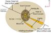 |
Fig. 1 Schematic (non-scaled) picture of the Z CMa system, as seen from Earth. The two stars are separated by ~ 0.1′′. (100 AU assuming a distance to Z CMa of 1150 pc.) The large jet associated to the primary, with an orientation of 245° is indicated by the black line, while the micro-jet, with an inclination of 235°, is indicated by the green dashed line. |
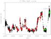 |
Fig. 2 Light curve of Z CMa. Black and red asterisks correspond to data from the American Association of Variable Star Observers (AAVSO) and the All Sky Automated Survey (ASAS) (Pojmanski 2002), respectively. Green asterisks correspond to data from the Czech Astronomical Society (CAS). |
The complex nature of this system makes imaging polarimetry a very interesting tool to better characterize it. While several authors have performed imaging polarimetry studies of circumstellar environments around young stars (e.g. Breger & Hardorp 1973; Bastien & Menard 1988; Close et al. 1997; Kuhn et al. 2001; Oppenheimer et al. 2008; Perrin et al. 2009), there are no imaging polarimetric observations of Z CMa to date. In this paper we present imaging polarimetry at optical wavelengths of Z CMa obtained with ExPo, the Extreme Polarimeter (see Keller 2006; Rodenhuis et al. 2008), currently a visitor instrument at the 4.2 m William Herschel Telescope (WHT). We describe the observations, the instrument, and the data reduction in Sect. 2. The image analysis and models are discussed in Sect. 3. The discussion and conclusion are given in Sects. 4 and 5, respectively.
2. Observations and data processing
Z CMa was observed on the 30 December, 2009 (night 1) and the 4 January, 2010 (night 2), during the third campaign (27/12/2009 − 04/01/2010) of ExPo as a visitor instrument at the WHT. The seeing during these two nights was fairly poor, with an average value of ~1.47′′. An unpolarized, diskless star (G 91-23) was observed on the night of 31 December, 2009 for comparison purposes. No filter was used during all these measurements, so the full optical range was covered (ExPo is sensitive to the wavelength range from 400 to 900 nm). Table 1 summarizes these observations. A set of calibration flat-fields was taken at the beginning and the end of each night, and a set of dark frames was taken at the beginning of each observation.
Summary of ExPo observations.
2.1. Instrument description
ExPo is a dual-beam imaging polarimeter working at optical wavelengths. It combines a fast modulating ferroelectric liquid crystal (FLC), a cube beamsplitter (BS) and an electron multiplying charge coupled device (EM-CCD). The FLC modulates the polarization state of the incoming light by 90° every 0.028 s, switching between two states “A” and “B”. By changing the voltage applied, the FLC modifies its state without having to rotate any part of the instrument1. The beamsplitter divides the incoming light into two beams (left and right beams) with orthogonal polarization states, which are then imaged onto two different regions of the 512 × 512 pixels EM-CCD. The current field of view of this instrument is 20′′ × 20′′, which is projected onto an area of the CCD of 256 × 256 pixels, resulting in a pixel size of 0.078′′/px.
At the end of one FLC cycle, four different images, Aleft, Aright, Bleft, Bright are produced. By subtracting the two simultaneous images recorded at the “A” and “B” states a “difference”, linearly polarized image, is produced:  A set of narrowband and broadband filters is implemented by a filter wheel, though none of these filters were used in the observations presented here. A standard ExPo observation comprises at least 4095 images (~2 min) recorded at one fixed FLC position. Once a set of measurements is finished, the FLC is rotated by 22.5°, and the procedure is repeated. At the end of the observation, four sets of measurements with the FLC oriented at 0°, 22.5°, 45°, and 67.5° are recorded during each observation.
2.2. Data analysis
Each one of the four images produced after one FLC cycle is finished are individually corrected of dark, bias, flat-field and cosmic rays. These images are then aligned by means of a cross-correlation algorithm. To increase the accuracy of this process, two different point spread function (PSF) templates, one for the left beam, and the other for the right beam, are produced during the reduction. The Aleft and Bleft images are then aligned accordingly to the coordinates of the maximum of the cross-correlation of each image with the left-beam template. The same process is repeated with the right-beam images and the right-beam template. For a detailed explanation of the data reduction techniques applied to the ExPo instrument, see Canovas et al. (2011). The short exposure time used by ExPo (0.028 s) allows us to minimize the tip-tilt error of the wavefront by properly aligning our images. The final full width at half maximum (FWHM) of our average PSF after centering is then ~1.2′′, which means an improvement of about ~20% with respect to the average seeing during our observations. A polarization image is obtained from a “double-difference” (Kuhn et al. 2001) by combining Eqs. (1) and (2):  (3)
(3) is a polarized, yet uncalibrated image. Because of the fast modulation of the FLC and the combination of two simultaneous images with opposite polarization states, most of the instrument systematic errors such as the highly static speckle noise (see, for instance, Racine et al. 1999; Sivaramakrishnan et al. 2002; Soummer et al. 2007) are removed (see for example Hinkley et al. 2009), allowing us to increase our sensitivity to faint, polarized features. The intensity image is calculated as the sum of the four images:
  (4)The instrumental polarization is removed by subtracting the average polarization degree in a circular area of radius 5 pixels (0.39′′), centered on the star, to the polarized images (for a detailed explanation of this process and its results when applied to ExPo see Canovas et al. 2011; Min et al. 2012). By doing this, we remove most of the instrumental polarization caused by the elements of the telescope + instrument system, but we also remove polarized light from the central star, in case the star itself is polarized. This method has been applied before by several authors (see for example Perrin et al. 2008; Quanz et al. 2011) when observing with different imaging polarimeters. The main advantage of this technique is that it allows us to trace the spatial variations in polarized intensity with high accuracy. As a collateral effect, the polarization degree measured with this instrument provides us with a lower limit of the true polarization degree in the observed targets.
Because ExPo does not have a de-rotator, sky rotation must be corrected for during the data reduction. To properly correct for this, not only a physical rotation of the image is needed (to preserve the north orientation when combining different datasets), but also a vectorial rotation of the Stokes Q and U images must be performed. After correcting for this, the Stokes parameters Q and U can be calculated in a reference frame fixed to the observed target. The sky polarization is corrected once the calibrated Stokes Q and U images are produced. To do this, the polarization of the sky is computed as the median of four different sky regions in the calibrated Stokes Q images. This value is then subtracted from these images, and the same process is repeated with the Stokes U images.
We produced two calibrated datasets from each observation. To produce Set 1 we combined and calibrated the images obtained with the FLC rotated at 0° and 22.5°, while Set 2 was produced by using the images obtained with the FLC rotated at 45° and 67.5°. Since in each observation the total amount of images observed in each one of the four FLC position is the same (see Table 1) both Set 1 and Set 2 have the same total exposure time. The polarized intensity (linearly polarized light) is calculated as  , and the degree of polarization as P = PI/I, where I is the total intensity. The polarization angle,
 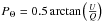 defines the orientation of the polarization plane. The error on the polarization angle depends on the error of the calibration process, but also on the region of the image where it is calculated. To minimize errors, the stokes Q and U images are binned with a 5 × 5 pixel (i.e. 0.39′′ × 0.39′′) box before PΘ is computed. Furthermore, PΘ is calculated only in the regions of the image with a signal-to-noise ratio (S/N) higher than 3 to reduce the error introduced by the noise. The accuracy of PΘ depends then on the position of the image at which it is calculated. For Z CMa, the maximum error we obtain for PΘ is of about ± 3.8° in the regions with a S/N higher than 3.
3. Results
A total amount of four calibrated datasets for Z CMa (two per night), and two calibrated datasets for the diskless, unpolarized star were obtained. Data from night 2 show a better S/N than data from night 1: the Moon was closer to Z CMa in night 1, increasing the amount of sky background noise. Therefore, we will focus our analysis on the first of the two datasets obtained during night 2, which is the set with higher S/N.
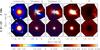 |
Fig. 3 Comparison of Z CMa (top row) and G 91-23 (unpolarized, diskless star, bottom row). North is up and east is left in all images. Starting from the left, the first column shows the total intensity image in logarithmic scale. The arrows indicate the position of different instrumental artifacts. The second and third column show the Stokes Q and U parameters, respectively. The polarized intensity (PI) is shown in the fourth column. G 91-23 shows a pattern caused by remnant, uncorrected, noise. Z CMa shows an extended, asymmetrical structure, with two extended features toward west and southwest. The fifth column shows the degree of polarization (P). The units of the color bars are given in CCD-counts, except in the case of P, where the degree (%) of polarization is shown. Our polarized images are calibrated in a reference system fixed to the observed object (see Sect. 2). |
Figure 3 shows a comparison between Z CMa and a diskless, unpolarized star (G 91-23). The first column, starting from the left side, shows the intensity image in logarithmic scale. The color scale in this case is chosen to enhance the instrumental artifacts in our images. In both images, the vertical arrow indicates the position of the ghost caused by the beamsplitter. The two horizontal arrows in the Z CMa image show the position of two ghosts caused by the FLC. The horizontal arrow in G 91-23 shows the position of one of the spiders of the telescope. The pattern produced by these spiders is clearly visible in this image. The inclined arrow indicates the effect of a non-perfect correction of the CCD-smearing effect. The two components of Z CMa appear unresolved in our images. The second and third columns show the stokes Q and U parameters, respectively. In the case of Z CMa, an extended, butterfly-like pattern is evident, while in the case of G 91-23 these two images are dominated by remnant noise. The fourth column shows the polarized intensity, PI, in which a very different pattern for each star is also evident. In the case of G 91-23, the PI image is dominated by the remnant noise that appears in the Q and U images. The noise from these images adds quadratically when computing PI, producing the observed pattern. In the case of Z CMa, PI shows a very strong asymmetry, with two extended features toward the west (to the right side of the image), and the southwest (to the bottom-right corner of the image). Because of the small separation of the two stars, it is impossible to resolve the dust cocoon around the primary in our images. Therefore, the extended polarized pattern that we see in Z CMa is probably caused by the circumbinary disk and infalling envelope. The fifth column shows the degree of polarization (P = PI/I) of Z CMa and the comparison star. The unpolarized star does not show any spatial structure but a centrosymmetric pattern. The polarized intensity, PI, which is by definition a positive quantity, is biased upward by the noise. On the other hand, the intensity I approaches zero when it approaches the edge of the image. These two effects combined produce what we see in the P image of the unpolarized star, where P increases its value when approaching the image’s edges. The image of Z CMa, however, shows again two polarization features, oriented toward west and southwest, respectively.
Further analysis shows that these two polarized structures appear at the same position in all observations of Z CMa. Z CMa was observed at a different altitude during night 2 when compared to night 1, but in all images we detect the same polarization features. If these two polarized features were caused by internal reflections or another instrumental artifact, they should appear in different positions when comparing images from night 1 with images from night 2. This rules out the possibility that these two features are caused by any instrumental or data processing artifact.
To reduce the noise in the polarization degree image, we have convolved the best dataset of our observations (night 2, Set 1) with a Gaussian kernel with a FWHM of 5 pixels (0.39′′). The resulting image is shown in Fig. 4. The left side of Fig. 4 shows PΘ. Only regions of the image with an S/N higher than 3 are displayed in this figure. The trajectory of the large jet (blueshifted component) associated to the Herbig star is indicated by the black line, at a position angle of 245°. The green line shows the position of the micro-jet associated to the FU Ori star, at a position angle of 235° (see Whelan et al. 2010). The position of the primary and the secondary is marked by the green cross at the center of the image. The right side of Fig. 4 shows the polarization degree image. The color scale is chosen to enhance the polarized features that appear in this image. The west side of Z CMa shows a polarized continuum with a degree of polarization of about 1.2% (the red colored regions). The orange and yellow regions indicated by the three arrows have a polarization degree higher than 1.5% The mean and standard deviation, σ, of P and PΘ of these three regions is shown in Table 2, together with results from previous spectropolarimetric observations of Z CMa.
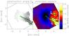 |
Fig. 4 Degree of polarization of Z CMa. North is up, east is left. The black and green lines show the trajectories of the large jet and micro-jet, respectively. The green cross shows the position of the binary; the separation of the stars is smaller than the size of the symbol. Left: PΘ is shown by the vectors. Only regions of the image with an S/N higher than 3 are displayed in this image. The length of the vectors is proportional to the local degree of polarization. Right: P image smoothed by convolution with a Gaussian kernel of 5 pixels. The black contours indicate the regions of the image where P is higher than 1.5%. The three arrows indicate the three regions of the image discussed in Sect. 4. |
4. Discussion
Z Cma was observed with ExPo during its last minimum. According to the current model (see Fig. 1), this implies that the primary star is obscured from sight, i.e., the medium is optically thick in the line of sight between the primary and us. At this stage, the primary contributes about 20% of the total flux at optical wavelengths, and its entire light is linearly polarized by the dust cocoon that surrounds it.
The process of removing the instrumental polarization, as explained in Sect. 2, will produce a systematic error in our measurements if the central star(s) is polarized. We cannot separate the instrumental polarization from the intrinsic polarization associated to Z CMa. The dependence of the instrumental polarization on the telescope pointing position prevents us from using the diskless star as an instrumental polarization calibrator: Z CMa and G 9143 were observed at different nights and telescope orientations. A characterization of the instrumental polarization would require a detailed model of the telescope + instrument system (see for example Witzel et al. 2011), and this is beyond of the scope of this paper. On the other hand, in the case of Z CMa the flux from the primary contributes up to 20% of the total flux at optical wavelengths, and is polarized (Whitney et al. 1993; Szeifert et al. 2010). The exact value of this polarization is not well known, with values ranging from 1.4% to 2.6%. Furthermore, this value is expected to change with the state of the dust cocoon surrounding the primary. As an extra source of error, the seeing severely affects the polarization degree by reducing its true value when the seeing increases. Because of all this our results must be taken as lower limits of the true intrinsic degree of polarization of the three different regions described below.
4.1. Region 1
The polarization angle (PΘ) inside this area is almost perpendicular to the direction of the blueshifted side of the parsec-sized jet, as is shown in the left image of Fig. 4. Moreover, this region follows the trajectory of the jet, as can be seen in the right image of Fig. 4. Whitney & Hartmann (1993) showed that the polarization pattern that we measure in this region, with PΘ perpendicular to the jet direction, is indeed the expected pattern when observing an infalling dust envelope with a cylindrical cavity carved out by a well-collimated jet.
Previous spectropolarimetric studies at optical wavelengths (Whitney et al. 1993; Szeifert et al. 2010) have reported a polarization angle perpendicular to the direction of the parsec-sized jet. The average PΘ that we measure in this region agree well with these previous observations, as is shown in Table 2. These results clearly suggest that this polarized feature is produced by scattering on the walls of the cavity carved out in the dusty envelope by the large jet. We therefore point to the large jet associated to the primary as the origin of the polarization pattern observed in region 1 of our images.
4.2. Region 2
This region shows the highest polarization degree in our Z CMa images. The trajectory of the micro-jet described by Whelan et al. (2010), 235°, is almost perpendicular to the polarization angle in this region: 144.9° ± 3.6°. As with the polarized feature in region 1, the polarized feature that we observe here is consistent with the polarization pattern predicted for an infalling envelope with empty cavities caused by a collimated outflow (Whitney & Hartmann 1993). This strongly points toward single scattering in the walls of a cavity carved out by this so-called micro-jet as the source of this polarized feature.
Our observations independently confirm the result from Whelan et al. (2010), and indicate that the micro-jet actually extends to a distance at least ten times longer than reported by these authors.
4.3. Region 3
The polarization angle of this area is very distinct from the polarization angles measured in previous observations. The average value of P inside this area is P = 1.6 ± 0.1% (3 sigmas above the background polarization), and the location of this region in our image is not close to any of the two jets associated to Z CMa. Therefore, we argue that this polarized feature is not related to any of the known jets. To explain its origin, we consider here the possibility of a hole in the dust cocoon surrounding the primary star pointing west. Some of the outbursts of Z CMa, as well as the spectropolarimetric measurements of this system, can be explained (Whitney et al. 1993; Szeifert et al. 2010) by the formation of holes in the dust cocoon surrounding the primary: if there is a hole in the dust cocoon in our line of sight, then an increase in the amount of light from the primary as well as a decrease on its polarization degree is expected.
To understand the impact of a hole in the optically thick dust cocoon surrounding the Herbig Be star, we used the MCMax radiative transfer code (Min et al. 2009) to model a pencil beam of light emerging from the dust cocoon that is scattered toward the observer by a surrounding infalling molecular cloud.
We are aware of the limitations of this simulation when we compared its results to our observations. Since we cannot quantify the instrumental polarization with sufficient accuracy, a direct comparison between our observations and the model can be misleading. Therefore, the primary goal of this modeling approach is to test wether a hole in the dust cocoon can produce a polarized feature similar to what we observe in region 3 rather than to provide detailed quantitative values for the parameters of the surrounding material.
4.3.1. Model setup
We simulated a binary system placed at a distance of 1150 pc (a value that agrees with the approximate distance to Z CMa), comprising an FU Ori star and a Herbig Be star. The basic parameters of the FU Ori star are taken from van den Ancker et al. (2004), resulting in an star of M = 3 M⊙, L = 27.5 L⊙. The luminosity of the embedded Herbig star is very poorly constrained in the literature, with values ranging from L = 3000 L⊙ (van den Ancker et al. 2004) to L = 310 000 L⊙ (Hartmann et al. 1989). For our model, we considered a Herbig Be star of M = 13 M⊙, L = 55 000 L⊙, which agrees well with the values obtained by Alonso-Albi et al. (2009), i.e., a star surrounded by an optically thick dust cocoon. The binary system is surrounded by a large infalling molecular envelope. The dust cocoon surrounding the Herbig Be star was modeled as an optically thick spherical shell with a hole with an opening angle (φ) varying from φ = 5° to φ = 10°. This cocoon is 50 AU in radius, starting at a distance of 20 AUs from the primary, which is the dust sublimation radius for this star. In this computation, three different orientations (with respect to the line of sight) of the hole in the dust cocoon were tested: + 45° (producing forward scattering), − 45° (producing backward scattering), and 90°. The infalling envelope was modeled as an optically thin spherical shell with the density distribution described by Dominik & Dullemond (2008), based on the work of Ulrich (1976) and Terebey et al. (1984). In this model, the infalling envelope is made from the remains of the collapse of a rotating cloud. The angle between a point on the envelope, the center of the envelope, and the rotational axis defines the polar coordinate θ. According to this model, the gas density ρ at a polar angle μ = cos θ and a distance to the center r is given by 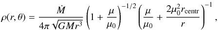 (5)where μ0 is the solution of the equation
 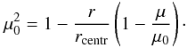 (6)Ṁ represents the infall rate and rcentr is the centrifugal radius, which here is fixed at a distance of 200 AU, as in the model of Dominik & Dullemond (2008). Four different values of Ṁ (1,2,4,8 × 10-7 M⊙ yr-1) were computed in our simulations. To easily distinguish between the different models we used the following notation: “model 1(5b)” refers to the model with Ṁ = 1 × 10⁻⁷ M⊙ yr-1, φ = 5, backward scattering; “model 4(10f)” refers to the model with Ṁ = 4 × 10⁻⁷ M⊙ yr-1, φ = 10, forward scattering, “model 4(10r)” refers to the model with Ṁ = 4 × 10⁻⁷ M⊙ yr-1, φ = 10, 90° scattering, and so on. The composition of the dust in the infalling envelope is described by Min et al. (2011), which is based on the solar composition inferred by Grevesse & Sauval (1998). The infalling envelope is composed by, in mass, 58% silicates, 18% iron sulphide, and 24% amorphous carbon. The dust size distribution follows the standard MRN size distribution (Mathis et al. 1977). In this distribution the number density of the grains is equated by the following power-law
 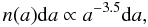 (7)where a is the radius of the grains, which ranges from 5 nm to 250 nm. The shape of the dust grains follows the distribution of hollow spheres (DHS, Min et al. 2005), assuming an “irregularity parameter” fmax = 0.8.
Mean values of P for the different models.
The radiative transfer images of the Z CMa system modeled by MCMax were then convolved with the modeled point spread function PSF of ExPo from Min et al. (2012). The PSF was modeled with an average seeing of 1.4′′ (as in our observations of Z CMa) and includes contributions from photon noise, readout noise, and instrumental polarization. To reproduce the ExPo observations, the exposure time used for these PSFs was 0.028 s. The resulting PSF is a speckle pattern, similar to what we obtain with ExPo observations. To simulate the effect of the instrument and the data processing, we proceeded as follows. We first produced a set of 100 statically independent, noiseless PSFs. The images produced by the MCMax code were then convolved with one simulated PSF. We then computed the photon noise associated to this new image. This noise was re-scaled to match the amplitude of the photon noise associated to a PSF with exposure time of 2.8 s. We then added this noise to the simulated image, and we repeated this process with all PSFs. At the end of the process we obtained a set of 100 different images, each one with the photon noise associated to an image of 2.8 s exposure time (or 100 images taken with 0.028 s of exposure time). This is roughly equivalent to computing 10 000 independent ExPo PSFs, but is much faster in terms of computing time. Instrumental polarization was added before the images were reduced with the ExPo pipeline described in Sect. 2.2 of this paper and Canovas et al. (2011). The resulting images produced after the reduction include accordingly both instrumental and data-processing effects, such as instrumental polarization or imperfect alignment. After reducing these simulated images, the averaged PSF has a FWHM of ~1.2′′, very similar to what we obtained after reducing our data. Both stars appear unresolved in the simulation, as in our observations. Finally, we reduced the noise in these images by convolving them with a Gaussian kernel of 5 pixels FWHM, as we did with our observations.
To compare with the real images and decide which model is the more realistic, we computed the mean value of the polarization degree in an area with the same size and shape as region 3 in Fig. 4. We also computed the background polarization (BP) as the mean of the degree of polarization inside of a half ring with inner radius rin = 4.1′′ and outer radius rout = 6.1′′ centered on the binary position. By doing this, we do not include the contribution of the polarized feature caused by the hole on the cocoon. This quantity systematically increases when increasing the mass infalling ratio, and it is practically insensitive to the size of the hole in the dust cocoon, as expected from our approach. Table 3 shows the average P of the final simulated image and the background polarization for each one of the models described above.
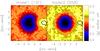 |
Fig. 5 Two models that reproduce the degree of polarization in an area equal to region 3 in Fig. 5. The model on the right produces an excess of background polarization, which translates into a bright ring around the (unpolarized) stars. The black lines are contouring an area equal to region 3 (see Fig. 4). |
We found that there are two models that produce an average polarization value similar to what we measured in region 3 of our image. These two models are “model 1 (10f)”, which produces P = 1.7%, and “model 2 (5b)”, which produces P = 1.6%. However, the model with the highest accretion rate fails when trying to reproduce the polarization background (BP = 1.3%). Because of the highest accretion rate, there is more dust contributing to the polarized background. This is clearly illustrated in Fig. 5. The bright, yellow blob that appears on the left image roughly resembles region 3 of Fig. 4.
There are too many unknowns of the Z CMa system to constrain all its details. Because of all the assumptions that we had to make during our modeling (i.e., hole geometry, dust shell geometry, dust composition, etc.), we must consider our results as a first indication only. However, within the uncertainties of our model, we obtain two results. First, the mass infall rate must be lower than Ṁ = 2 × 10⁻⁷ M⊙ yr-1 to fit our model. Second, and perhaps more important, a new hole in the dust cocoon surrounding the primary can explain the polarized feature observed in region 3 of our images.
5. Conclusions
Our measurements, obtained with ExPo after the 2008 outburst, show three different features in polarization. Two of them, labeled here “region 2” and “region 3” have not been reported before. This is thanks to the high polarimetric sensitivity of ExPo, and the different nature of our data, which employ imaging polarimetry and not spectropolarimetry. We interpret our data as new evidence of the presence of holes in the dust cocoon that surrounds the primary star: our simulation of the effects of one hole in the dust cocoon can reproduce the polarized feature observed in region 3.
The polarized feature labeled here region 1 in Fig. 5 shows an average polarization angle of PΘ = 155.4° ± 3.9°, which is perpendicular to the direction of the large jet and is very similar to the value found by Whitney et al. (1993) and Szeifert et al. (2010). The orientation of PΘ indicates that this polarized feature is consistent with scattering on the walls of a cavity carved out by the large jet, whose trajectory is perpendicular to PΘ. Benisty et al. (2010) showed evidence of a tilted accretion disk around the primary by analyzing the Brγ emission line produced on the hot gas around this star. If this is the case, then this disk must be inside of the dust cocoon that surrounds this star to explain all the previous evidence of a dust cocoon around the primary.
The average polarization angle in region 2 is perpendicular to the trajectory of the micro-jet. This strongly suggests that this feature is caused by single scattering that originated in the walls of a cavity carved out by this jet. The results from Whelan et al. (2010) indicate that this jet extends up to a distance of 0.5′′ from the FU Ori star, while the polarized feature that we observe appears at a distance of ≈ 5′′ from the FU Ori star. This indicates that this micro-jet actually extends to sizes much larger than reported before.
Our analysis suggests that the polarized feature that we detect in region 3 in Fig. 5 is caused by a hole in the dust cocoon surrounding the primary star. This idea is not new and has been used to explain the variability and polarimetric properties of this system. However, in previous discussions, the hole in the cocoon was assumed to be in our line of sight to explain some of the outbursts of Z CMa. To fit our observations, a hole with a different orientation must be used: a hole in one side of the cocoon can produce a pencil beam of light (like a lighthouse) that will be scattered to our line of sight, producing a polarized signature similar to what we observe in region 3. To simulate this, we ran different models with different hole sizes, orientations, and different mass infall rates for the surrounding infalling envelope. We conclude that a hole in the dust cocoon can produce a polarized beam of light that explains the polarized feature observed in region 3. According to our calculations and models, the mass infall rate of the infalling envelope cannot be higher than Ṁ = 2 × 10⁻⁷ M⊙ yr-1. Given the error bars on the luminosity of the primary star (see, for instance, Monnier et al. 2005), together with the many assumptions made in our model, we take this value as a first approximation. The derived infall rate scales inversely with the luminosity of the system; therefore, if we are overestimating the luminosity of the Herbig Be star, we are underestimating the infall rate, and vice-versa.
Region 3 requires more observations for a proper analysis of our results. The nature of the dust cocoon around the primary remains a puzzle, with many open questions about it, such as its size or grain composition. The source of these holes and/or variability in the dust cocoon remains still unknown, but one possible explanation might be related to the nature of this system: given the small separation between the primary and the secondary, their gravitational interaction might affect the dust cocoon around the primary (as an example of the effect of binarity over circumstellar disk sizes, see Artymowicz & Lubow 1994).
Z CMa is a system with an extremely high variability. However, the different nature of the data discussed by previous authors (Whitney et al. 1993; Szeifert et al. 2010) and ours leaves no room to discuss this variability in terms of the observations presented here and the previous ones. On the other hand, the Keplerian timescale2 of a dust particle orbiting an M = 13 M⊙ star at a distance equal to the sublimation radius (20 AU in this case) is approximately 24 years, and about 100 years when the distance to the star is 50 AU. Therefore, one might expect to measure variability caused by the movement of the dust cocoon around the primary on timescales of years to decades.
A characterization of the dust properties of this system will help to constrain the huge error bars associated to the luminosity of the primary star, helping to solve some of the unknowns of this complex system. Furthermore, the determination of the infall rate could help to explain mechanisms that produce the extreme accretion rates measured for the FU Ori star (see Hartmann & Kenyon 1996).
Z CMa is a very interesting system to perform imaging polarimetry studies on. If the dust cocoon around the primary is rapidly modifying its geometry, then new holes (i.e., new polarized features) are expected to appear. According to our results, this could happen on timescales of about a few years. Future observations of this system with imaging polarimeters such as ExPo or SPHERE will provide crucial information helping to understand the environment of Z CMa.
The FLC can actually modify its state at much higher rates than the 35 Hz used by ExPo. The exposure time in this instrument is currently limited by the EM-CCD, which is unable to operate at exposure times shorter than 0.028 s.
The Keplerian timescale indicates the orbital period around a central object of mass M ⋆ . It can be approximated as  , where R is the orbital radius, e is the eccentricity of the orbit and G is the general constant of gravity.
Acknowledgments
The authors thank the anonymous referee for providing very constructive comments, which significantly helped to improve the paper. We are also grateful to the staff at the William Herschel Telescope for their help during the observations. H.C.C. acknowledges support from Millenium Science Initiative, Chilean Ministry of Economy, Nucleus P10-022-F.
References
- Alonso-Albi, T., Fuente, A., Bachiller, R., et al. 2009, A&A, 497, 117 [NASA ADS] [CrossRef] [EDP Sciences] [Google Scholar]
- Artymowicz, P., & Lubow, S. H. 1994, ApJ, 421, 651 [NASA ADS] [CrossRef] [Google Scholar]
- Barth, W., Weigelt, G., & Zinnecker, H. 1994, A&A, 291, 500 [NASA ADS] [Google Scholar]
- Bastien, P., & Menard, F. 1988, ApJ, 326, 334 [NASA ADS] [CrossRef] [Google Scholar]
- Beckwith, S. V. W., & Sargent, A. I. 1991, ApJ, 381, 250 [NASA ADS] [CrossRef] [Google Scholar]
- Benisty, M., Malbet, F., Dougados, C., et al. 2010, A&A, 517, L3 [NASA ADS] [CrossRef] [EDP Sciences] [Google Scholar]
- Breger, M., & Hardorp, J. 1973, ApJ, 183, L77 [NASA ADS] [CrossRef] [Google Scholar]
- Canovas, H., Rodenhuis, M., Jeffers, S. V., Min, M., & Keller, C. U. 2011, A&A, 531, A102 [NASA ADS] [CrossRef] [EDP Sciences] [Google Scholar]
- Clariá, J. J. 1974, A&A, 37, 229 [NASA ADS] [Google Scholar]
- Close, L. M., Roddier, F., Hora, J. L., et al. 1997, ApJ, 489, 210 [NASA ADS] [CrossRef] [Google Scholar]
- Dominik, C., & Dullemond, C. P. 2008, A&A, 491, 663 [NASA ADS] [CrossRef] [EDP Sciences] [Google Scholar]
- Fischer, O., Stecklum, B., & Leinert, C. 1998, A&A, 334, 969 [NASA ADS] [Google Scholar]
- Garcia, P. J. V., Thiébaut, E., & Bacon, R. 1999, A&A, 346, 892 [NASA ADS] [Google Scholar]
- Grevesse, N., & Sauval, A. J. 1998, Space Sci. Rev., 85, 161 [NASA ADS] [CrossRef] [Google Scholar]
- Haas, M., Christou, J. C., Zinnecker, H., Ridgway, S. T., & Leinert, C. 1993, A&A, 269, 282 [NASA ADS] [Google Scholar]
- Hartmann, L., & Kenyon, S. J. 1996, ARA&A, 34, 207 [NASA ADS] [CrossRef] [EDP Sciences] [MathSciNet] [Google Scholar]
- Hartmann, L., Kenyon, S. J., Hewett, R., et al. 1989, ApJ, 338, 1001 [NASA ADS] [CrossRef] [Google Scholar]
- Herbst, W., Racine, R., & Warner, J. W. 1978, ApJ, 223, 471 [NASA ADS] [CrossRef] [Google Scholar]
- Hinkley, S., Oppenheimer, B. R., Soummer, R., et al. 2009, ApJ, 701, 804 [NASA ADS] [CrossRef] [Google Scholar]
- Ibragimov, M. A., & Shevchenko, V. S. 1990, in Conf. classical Be stars and Ae/Be Herbig stars, ed A. Kh. Mamatkazina (Alma Ata) [Google Scholar]
- Kaltcheva, N. T., & Hilditch, R. W. 2000, MNRAS, 312, 753 [NASA ADS] [CrossRef] [Google Scholar]
- Keller, C. U. 2006, in Proc. SPIE, 6269, 62690 [Google Scholar]
- Koresko, C. D., Beckwith, S. V. W., Ghez, A. M., Matthews, K., & Neugebauer, G. 1991, AJ, 102, 2073 [NASA ADS] [CrossRef] [Google Scholar]
- Kuhn, J. R., Potter, D., & Parise, B. 2001, ApJ, 553, L189 [NASA ADS] [CrossRef] [Google Scholar]
- Malbet, F., Rigaut, F., Bertout, C., & Lena, P. 1993, A&A, 271, L9 [NASA ADS] [Google Scholar]
- Mathis, J. S., Rumpl, W., & Nordsieck, K. H. 1977, ApJ, 217, 425 [NASA ADS] [CrossRef] [Google Scholar]
- Min, M., Hovenier, J. W., & de Koter, A. 2005, A&A, 432, 909 [NASA ADS] [CrossRef] [EDP Sciences] [Google Scholar]
- Min, M., Dullemond, C. P., Dominik, C., de Koter, A., & Hovenier, J. W. 2009, A&A, 497, 155 [NASA ADS] [CrossRef] [EDP Sciences] [Google Scholar]
- Min, M., Dullemond, C. P., Kama, M., & Dominik, C. 2011, Icarus, 212, 416 [NASA ADS] [CrossRef] [Google Scholar]
- Min, M., Canovas, H., Mulders, G. D., & Keller, C. U. 2012, A&A, 537, A75 [NASA ADS] [CrossRef] [EDP Sciences] [Google Scholar]
- Monnier, J. D., Millan-Gabet, R., Billmeier, R., et al. 2005, ApJ, 624, 832 [NASA ADS] [CrossRef] [Google Scholar]
- Oppenheimer, B. R., Brenner, D., Hinkley, S., et al. 2008, ApJ, 679, 1574 [Google Scholar]
- Perrin, M. D., Graham, J. R., & Lloyd, J. P. 2008, PASP, 120, 555 [NASA ADS] [CrossRef] [Google Scholar]
- Perrin, M. D., Vacca, W. D., & Graham, J. R. 2009, AJ, 137, 4468 [NASA ADS] [CrossRef] [Google Scholar]
- Poetzel, R., Mundt, R., & Ray, T. P. 1989, A&A, 224, L13 [NASA ADS] [Google Scholar]
- Pojmanski, G. 2002, Acta Astron., 52, 397 [NASA ADS] [Google Scholar]
- Quanz, S. P., Schmid, H. M., Geissler, K., et al. 2011, ApJ, 738, 23 [NASA ADS] [CrossRef] [Google Scholar]
- Racine, R., Walker, G. A. H., Nadeau, D., Doyon, R., & Marois, C. 1999, PASP, 111, 587 [NASA ADS] [CrossRef] [Google Scholar]
- Rodenhuis, M., Canovas, H., Jeffers, S. V., & Keller, C. U. 2008, in Proc. SPIE, 7014, 70146 [Google Scholar]
- Sivaramakrishnan, A., Lloyd, J. P., Hodge, P. E., & Macintosh, B. A. 2002, ApJ, 581, L59 [NASA ADS] [CrossRef] [Google Scholar]
- Soummer, R., Ferrari, A., Aime, C., & Jolissaint, L. 2007, ApJ, 669, 642 [NASA ADS] [CrossRef] [Google Scholar]
- Szeifert, T., Hubrig, S., Schöller, M., et al. 2010, A&A, 509, L7 [NASA ADS] [CrossRef] [EDP Sciences] [Google Scholar]
- Terebey, S., Shu, F. H., & Cassen, P. 1984, ApJ, 286, 529 [NASA ADS] [CrossRef] [Google Scholar]
- Tessier, E., Bouvier, J., & Lacombe, F. 1994, A&A, 283, 827 [NASA ADS] [Google Scholar]
- Thiebaut, E., Bouvier, J., Blazit, A., et al. 1995, A&A, 303, 795 [NASA ADS] [Google Scholar]
- Ulrich, R. K. 1976, ApJ, 210, 377 [NASA ADS] [CrossRef] [Google Scholar]
- van den Ancker, M. E., Blondel, P. F. C., Tjin A Djie, H. R. E., et al. 2004, MNRAS, 349, 1516 [NASA ADS] [CrossRef] [Google Scholar]
- Velázquez, P. F., & Rodríguez, L. F. 2001, Rev. Mex. Astron. Astrofis., 37, 261 [NASA ADS] [Google Scholar]
- Whelan, E. T., Dougados, C., Perrin, M. D., et al. 2010, ApJ, 720, L119 [NASA ADS] [CrossRef] [Google Scholar]
- Whitney, B. A., & Hartmann, L. 1993, ApJ, 402, 605 [NASA ADS] [CrossRef] [Google Scholar]
- Whitney, B. A., Clayton, G. C., Schulte-Ladbeck, R. E., et al. 1993, ApJ, 417, 687 [NASA ADS] [CrossRef] [Google Scholar]
- Witzel, G., Eckart, A., Buchholz, R. M., et al. 2011, A&A, 525, A130 [NASA ADS] [CrossRef] [EDP Sciences] [Google Scholar]
All Tables
All Figures
|
Fig. 1 Schematic (non-scaled) picture of the Z CMa system, as seen from Earth. The two stars are separated by ~ 0.1′′. (100 AU assuming a distance to Z CMa of 1150 pc.) The large jet associated to the primary, with an orientation of 245° is indicated by the black line, while the micro-jet, with an inclination of 235°, is indicated by the green dashed line. |
| In the text | |
|
Fig. 2 Light curve of Z CMa. Black and red asterisks correspond to data from the American Association of Variable Star Observers (AAVSO) and the All Sky Automated Survey (ASAS) (Pojmanski 2002), respectively. Green asterisks correspond to data from the Czech Astronomical Society (CAS). |
| In the text | |
|
Fig. 3 Comparison of Z CMa (top row) and G 91-23 (unpolarized, diskless star, bottom row). North is up and east is left in all images. Starting from the left, the first column shows the total intensity image in logarithmic scale. The arrows indicate the position of different instrumental artifacts. The second and third column show the Stokes Q and U parameters, respectively. The polarized intensity (PI) is shown in the fourth column. G 91-23 shows a pattern caused by remnant, uncorrected, noise. Z CMa shows an extended, asymmetrical structure, with two extended features toward west and southwest. The fifth column shows the degree of polarization (P). The units of the color bars are given in CCD-counts, except in the case of P, where the degree (%) of polarization is shown. Our polarized images are calibrated in a reference system fixed to the observed object (see Sect. 2). |
| In the text | |
|
Fig. 4 Degree of polarization of Z CMa. North is up, east is left. The black and green lines show the trajectories of the large jet and micro-jet, respectively. The green cross shows the position of the binary; the separation of the stars is smaller than the size of the symbol. Left: PΘ is shown by the vectors. Only regions of the image with an S/N higher than 3 are displayed in this image. The length of the vectors is proportional to the local degree of polarization. Right: P image smoothed by convolution with a Gaussian kernel of 5 pixels. The black contours indicate the regions of the image where P is higher than 1.5%. The three arrows indicate the three regions of the image discussed in Sect. 4. |
| In the text | |
|
Fig. 5 Two models that reproduce the degree of polarization in an area equal to region 3 in Fig. 5. The model on the right produces an excess of background polarization, which translates into a bright ring around the (unpolarized) stars. The black lines are contouring an area equal to region 3 (see Fig. 4). |
| In the text | |
Current usage metrics show cumulative count of Article Views (full-text article views including HTML views, PDF and ePub downloads, according to the available data) and Abstracts Views on Vision4Press platform.
Data correspond to usage on the plateform after 2015. The current usage metrics is available 48-96 hours after online publication and is updated daily on week days.
Initial download of the metrics may take a while.