| Issue |
A&A
Volume 542, June 2012
|
|
|---|---|---|
| Article Number | A62 | |
| Number of page(s) | 11 | |
| Section | Stellar structure and evolution | |
| DOI | https://doi.org/10.1051/0004-6361/201219132 | |
| Published online | 07 June 2012 | |
Effects of thermohaline instability and rotation-induced mixing on the evolution of light elements in the Galaxy: D, 3He and 4He
1 Geneva Observatory, University of Geneva, Chemin des Maillettes 51, 1290 Versoix, Switzerland
e-mail: This email address is being protected from spambots. You need JavaScript enabled to view it.
2 INAF – Bologna Observatory, via Ranzani 1, 40127 Bologna, Italy
3 IRAP, CNRS UMR 5277, Université de Toulouse, 14, Av. E.Belin, 31400 Toulouse, France
4 Leibniz – Institut für Astrophysik Potsdam (AIP), An der Sternwarte 16, 14482 Potsdam, Germany
5 Physics Department, Trieste University, via Tiepolo 11, 34143 Trieste, Italy
6 INAF-Trieste Observatory, via Tiepolo 11, 34143 Trieste, Italy
Received: 28 February 2012
Accepted: 8 April 2012
Abstract
Context. Recent studies of low- and intermediate-mass stars show that the evolution of the chemical elements in these stars is very different from that proposed by standard stellar models. Rotation-induced mixing modifies the internal chemical structure of main sequence stars, although its signatures are revealed only later in the evolution when the first dredge-up occurs. Thermohaline mixing is likely the dominating process that governs the photospheric composition of low-mass red giant branch stars and has been shown to drastically reduce the net 3He production in these stars. The predictions of these new stellar models need to be tested against galaxy evolution. In particular, the resulting evolution of the light elements D, 3He and 4He should be compared with their primordial values inferred from the Wilkinson Microwave Anisotropy Probe data and with the abundances derived from observations of different Galactic regions.
Aims. We study the effects of thermohaline mixing and rotation-induced mixing on the evolution of the light elements in the Milky Way.
Methods. We compute Galactic evolutionary models including new yields from stellar models computed with thermohaline instability and rotation-induced mixing. We discuss the effects of these important physical processes acting in stars on the evolution of the light elements D, 3He, and 4He in the Galaxy.
Results. Galactic chemical evolution models computed with stellar yields including thermohaline mixing and rotation fit better observations of 3He and 4He in the Galaxy than models computed with standard stellar yields.
Conclusions. The inclusion of thermohaline mixing in stellar models provides a solution to the long-standing “3He problem” on a Galactic scale. Stellar models including rotation-induced mixing and thermohaline instability reproduce also the observations of D and 4He.
Key words: Galaxy: evolution / galaxies: abundances / galaxies: formation
© ESO, 2012
1. Introduction
Understanding the evolution of the light elements deuterium (D), helium-3 (3He), and helium-4 (4He) hinges on the comprehension of several astrophysical processes and links together different branches of physics and cosmology. D, 3He, and 4He are all synthesized in astrophysically relevant quantities during Big Bang nucleosynthesis (BBN; Peebles 1966; Wagoner et al. 1967). In the absence of any other realistic production channel (Epstein et al. 1976; Prodanović & Fields 2003), the abundance of D in galaxies smoothly decreases in time as gas cycles through stars. 3He and 4He, instead, have a more complex history, since they are both produced and destroyed in stars.
The sensitivity of the predicted BBN abundance of D, (D/H)P, to the baryon-to-photon ratio, ηB, coupled with its straightforward galactic evolution, has long made this element be the “baryometer” of choice (Reeves et al. 1973). In the nineties, the controversial assessment of the primordial abundance of D from observations of high-redshift clouds (e.g. Songaila et al. 1994; Burles & Tytler 1998), probing an almost unevolved medium, led researchers to resort to detailed Galactic chemical evolution (GCE) modelling in order to constrain the pre-Galactic D abundance and, hence, the value of ηB. It was shown that any reasonable GCE model results in moderate local D astration, by less than a factor of three (Steigman & Tosi 1992; Edmunds 1994; Galli et al. 1995; Dearborn et al. 1996; Prantzos 1996; Tosi et al. 1998; Chiappini et al. 2002). Assuming that the local present-day abundance of D is well known, this provided a stringent bound to (D/H)P and, hence, a test for BBN theories. Chemical evolution models able to reproduce the majority of the observational constraints for the Milky Way firmly ruled out the highest values of (D/H)P by Songaila et al. (1994). In particular, the values of (D/H)P and ηB suggested by Tosi (2000) and Chiappini et al. (2002) turned out to be in very good agreement with the ones determined from the analysis of the first Wilkinson Microwave Anisotropy Probe (WMAP) data (Bennett et al. 2003; Spergel et al. 2003).
Abundances of deuterium, 3He, and 4He at different epochs.
Indeed, the first release of results from WMAP made us enter a new precision era for cosmology – ηB is now known with exquisite accuracy. Converging measurements of D abundances in remote gas clouds lead to (D/H)P = (2.8 ± 0.2) × 10-5 (Pettini et al. 2008), a value consistent, within the errors, with the primordial D abundance predicted by the standard model of cosmology with parameters fixed by WMAP data (e.g. Cyburt et al. 2008; Coc et al. 2004, see Table 1). The remarkable homogeneity of D abundances at high redshifts, however, clashes with the unexpectedly large scatter in D/H revealed by determinations of relatively local D abundances (Vidal-Madjar et al. 1998; Jenkins et al. 1999; Sonneborn et al. 2000; Hébrard et al. 2002; Oliveira & Hébrard 2006). The observed dispersion can be reconciled with the predictions on D evolution from standard GCE models by taking into account two short-term, small-scale phenomena: D depletion onto dust grains and localized infall of primordial gas (Romano et al. 2006; Steigman et al. 2007; Romano 2010).
As far as 3He is concerned, Iben (1967) and Truran & Cameron (1971) first showed that large amounts of this element are produced by low-mass stars (M ≃ 1–3 M⊙) in the ashes of hydrogen burning by the p-p cycle on the main sequence. Problems arised soon, when Rood et al. (1976) incorporated these yields in models of GCE and came out with predicted 3He abundances orders of magnitude higher than the observed ones in the Galaxy. Indeed, the nearly constancy of the 3He abundance with both time and position within the Galaxy (e.g. Bania et al. 2002) rather implies a negligible production of this element in stars, at variance with predictions from standard stellar models. It was then advocated that some non-standard mechanisms are acting in a major fraction of low-mass stars, which prevents the fresh 3He from surviving and being ejected in the interstellar medium (ISM; Rood et al. 1984). For instance, extra mixing was also invoked in order to explain other abundance anomalies like the carbon isotopic ratio in red giants (Charbonnel 1995; Hogan 1995; Charbonnel & Do Nascimento 1998; see also Eggleton et al. 2006, 2008). The first 3He stellar yields for low-mass stars computed with “ad hoc” extra-mixing (i.e., not related to a physical mechanism, see Sect. 2.2.2) became available with the work of Boothroyd & Sackmann (1999). Galli et al. (1997); Palla et al. (2000); Chiappini et al. (2002) implemented those yields, accounting for the dependency of the helium-3 production/destruction on the stellar mass, metallicity and initial D abundances. It was shown that chemical evolution models which account for about 90% of low-mass stars undergoing extra-mixing led to a good agreement with the Proto Solar Cloud (PSC) observations as well as with the observed gradient along the disk.
The physical process responsible for the extra-mixing has possibly been recently identified. Charbonnel & Zahn (2007b) have shown indeed that thermohaline instability, when modelled with a simple prescription based on linear stability analysis, leads to a drastic reduction of 3He production in low-mass, low-metallicity red giant stars. However a couple of planetary nebulae, namely NGC 3242 and J320, have been found to behave classically (see Bania et al. 2010): slightly more massive than the Sun, they are currently returning fresh 3He to the ISM, in agreement with standard predictions (Rood et al. 1992; Galli et al. 1997; Balser et al. 1999, 2006). To reconcile the 3He/H measurements in Galactic HII regions with the high values of 3He in NGC 3242 and J320, Charbonnel & Zahn (2007a) proposed that thermohaline mixing is inhibited by a fossil magnetic field in red giant branch (RGB) stars that are descendants of Ap stars. The percentage of such stars is about 2–10% of all A-type objects. This number agrees with the fact that about 4% of low-mass evolved stars (including NGC 3242) exhibit standard suface abundances as depicted by their carbon isotopic ratios (Charbonnel & Do Nascimento 1998). Grids of 3He yields from stellar models taking into account thermohaline instability, as well as rotational mixing, are presented in Lagarde et al. (2011). These are suitable for use in GCE studies such as the one presented here.
The scarce determinations of reliable 4He abundances in the Galaxy (Balser et al. 2010; Peimbert et al. 2010), together with the steadiness of GCE model predictions on the evolution of 4He when adopting different stellar yields (e.g. Chiappini et al. 2002; Romano et al. 2010), have given this element little attention in GCE studies.
In this paper, we deal with the evolution of D, 3He, and 4He in the solar vicinity, as well as their distributions across the Galactic disc. The production of 3He is strictly related to the destruction of D and the production of 4He. Therefore, these elements are considered all together. The main novelty of the present work is the new nucleosynthesis prescriptions for the synthesis of 3He and 4He in low-mass stars (masses below 6 M⊙). Here we present, for the first time, chemical evolution models for 3He computed with stellar yields from non-standard stellar models that include both rotation-induced and thermohaline mixing (Charbonnel & Zahn 2007a; Charbonnel & Lagarde 2010; Lagarde et al. 2011). As we will show in the next sections, these yields bring chemical evolution model predictions into agreement with the Galactic 3He data without the necessity of assuming “ad hoc” fractions of extra-mixing among low-mass stars.
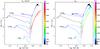 |
Fig. 1 Theoretical evolutionary tracks in the HR diagram for the 1.5 M⊙, 3.0 M⊙, and 6.0 M⊙ models at solar metallicity following the standard prescription (left panel); and including rotation-induced mixing and thermohaline instability (right panel), from the pre-main sequence up to the end of the TP-AGB phase. Colours depict the mass fraction of 3He at the stellar surface as indicated on the right, with the arrows showing the initial 3He and 3He + 2H content assumed at birth. |
The layout of the paper is as follows. In Sect. 2 we discuss the production/destruction channels of D, 3He, and 4He in stars in light of new generation stellar models that take into account rotation-induced mixing and thermohaline instability. A comparison with stellar yields predictions from the literature is presented. In Sect. 3 we describe the adopted GCE model. In Sect. 4 we discuss our results on the evolution of the light elements in the Galaxy. In particular, we try to put constraints on the uncertain parameters of stellar evolution through a comparison of the model predictions with the relevant data. We draw our conclusions in Sect. 5.
2. Stellar nucleosynthesis of light elements from new generation models for low- and intermediate-mass stars
In a series of papers (Charbonnel & Lagarde 2010; Lagarde et al. 2011, 2012, hereinafter Papers I, II and III, respectively; see also Charbonnel & Zahn 2007b,a), we discuss the impact of rotation-induced mixing and thermohaline instability on the structure, evolution, nucleosynthesis and yields, as well as on the asteroseismic and chemical properties of low- and intermediate-mass stars at various metallicities. A detailed description of the input physics of the models is given in Paper III. Rotation-induced mixing is treated using the complete formalism developed by Zahn (1992) and Maeder & Zahn (1998) (see for more details, Papers I, II, III). In these stellar models, we consider that thermohaline instability develops as long thin fingers with the aspect ratio consistent with predictions by Ulrich (1972) and confirmed by the laboratory experiments (Krishnamurti 2003). We note that this value is higher than obtained by current 2D and 3D numerical simulations (Denissenkov 2010; Denissenkov & Merryfield 2011; Rosenblum et al. 2011; Traxler et al. 2011). Before a final word on this discrepancy comes from future numerical simulations in realistic stellar conditions, we adopt an aspect ration (i.e., maximum length relative to their diameter) of 5, which nicely accounts for the observed chemical properties of red giant stars. These new generation stellar models account very nicely for main-sequence and RGB abundance patterns observed in field and open cluster stars over the mass and metallicity range covered, as shown in Paper I and in Charbonnel & Zahn (2007b). In this section we briefly summarize their characteristics as far as the nucleosynthesis of light elements is concerned.
2.1. Deuterium
Deuterium burns by proton-captures at low temperature during the pre-main sequence (Reeves et al. 1973). Therefore, it is totally destroyed in stellar interiors and the corresponding net yields are negative whatever the mass and metallicity of the star, as in the case of standard stellar models.
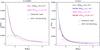 |
Fig. 2 Mass fraction of 3He at the stellar surface at the end of the second dredge-up as a function of initial stellar mass in standard models (solid lines and triangles) and in models including various prescriptions for mixing in the radiative regions (dashed lines), at two metallicities (Z = 0.0001 and Z = 0.014; left and right panels, respectively). The predictions are from Dearborn et al. (1996, DST96, blue line), Boothroyd & Sackmann (1999, BS99, at the RGB tip, magenta lines), Weiss et al. (1996, WWD96, red triangles), and Lagarde et al. (2011, LC11, black lines). The initial abundances of 3He adopted at the zero age main sequence by the different authors are given on the top right corner of each panel. |
2.2. Helium-3
2.2.1. Impact of rotation-induced mixing and thermohaline instability on model predictions
Paper II describes in detail the behaviour of 3He both in the standard case and in our models including thermohaline instability and rotation-induced mixing. Figure 1 shows the theoretical evolution of the 3He surface abundance along the evolutionary tracks in the HR diagram for the models of 1.5, 3.0, and 6.0 M⊙ at solar metallicity that take into account these two processes. The colour coding in mass fraction is given on the right, with the initial values of 3He and D + 3He indicated by the arrows. Evolution is shown from the pre-main sequence along the Hayashi track up to the end of the thermally-pulsing asymptotic giant branch (TP-AGB) phase. We see the changes in 3He surface abundance due to D-burning on the pre-main sequence except in the 6.0 M⊙ model whose convective envelope withdraws very quickly at the beginning of that phase allowing to the preservation of pristine D in a very thin external layer. 3He is then produced in low- and intermediate-mass stars during the main sequence through the pp-chains and subsequently dredged-up when the stars move towards the RGB. On the 1.5 M⊙ track one sees the effect of rotation-induced mixing that already brings fresh 3He towards the stellar surface while the star is on the main sequence (on the contrary, in the standard case the surface abundance of 3He remains constant on the main sequence and starts changing only at the very base of the RGB due to the first dredge-up). However, as discussed in Paper II rotation-induced mixing is found to lower the total 3He production compared to the standard case over the whole mass and metallicity range scrutinized, and to decrease the upper mass limit at which stars destroy this element (see Fig. 5 in Paper II). Additionally, for low-mass stars (M ≤ 2–2.2 M⊙) thermohaline mixing occurring during the RGB phase beyond the bump and on the TP-AGB leads to the destruction of part of the freshly produced 3He while accounting for the observed surface abundance anomalies of other chemicals (i.e., lithium and nitrogen, as well as carbon isotopic ratio; see also Charbonnel & Zahn 2007b); the associated decrease of surface 3He is clearly seen for the 1.5 M⊙ model in Fig.1 (right panel). Therefore, although low-mass stars remain net 3He producers, their contribution to the Galactic evolution of this element is much lower than in the standard case. It was also shown in Paper II that thermohaline mixing leads to 3He depletion during the TP-AGB phase for stars with masses up to ~4 M⊙ (see the 3 M⊙ track in the figure). In more massive intermediate-mass stars, 3He is further destroyed through hot-bottom burning on the TP-AGB. Finally, this figure shows that the lower the mass of the star, the higher the surface abundance of 3He at the end of the TP-AGB. The global impact of rotation-induced mixing and thermohaline instability on the net 3He yields from low- and intermediate-mass stars of various metallicities is summarized in Fig. 9 and in Tables 1 to 4 of Paper II (see also Fig. 2 discussed below).
2.2.2. Comparison with other stellar models
In Fig. 2 we show the mass fraction of 3He at the end of the second dredge-up as a function of the initial stellar mass at two metallicities (Z = 0.0001 and 0.014; left and right panels, respectively) from our models (black lines; see Paper II). A comparison is made with model predictions from the literature (coloured lines and filled triangles).
Our standard predictions (full lines) are in very good agreement with those from Dearborn et al. (1996), Boothroyd & Sackmann (1999), and Weiss et al. (1996). For the reasons given in Sect. 2.2.1 they are higher than in the case including rotation-induced mixing and thermohaline instability (dashed black lines). Let us note that thermohaline mixing on the TP-AGB leads to further decrease of the 3He mass fraction at the stellar surface (reduction of 64, 83, and 19% in the [1.25 M⊙, Z⊙], [0.85 M⊙, Z = 0.0001], and [2.0 M⊙, Z⊙ and Z = 0.0001] models, respectively; see Paper II).
In Fig. 2 we also plot the predictions at the end of the second dredge-up for the models of Boothroyd & Sackmann (1999, hereafter BS99) that include parametric mixing below the base of the convective envelope of RGB stars (the so-called “conveyor-belt” circulation and the associated “cool bottom processing”, CBP; dashed magenta lines). In BS99 post-processing computations, the mixing is not related to any physical mechanism. Rather, the depth of the mixed zone is a free parameter that corresponds to the difference ΔlogT between the temperature at the base of the hydrogen-burning shell and that at the base of the assumed mixed zone. BS99 assumed that the value of Δlog T remains constant along the RGB, and this free parameter was calibrated in order to reproduce the observed carbon isotopic ratio of clump stars in M 67. We note that the fixed Δlog T value used by BS99 leads to shallower mixing just after the RGB bump than what we get when considering thermohaline instability as the physical mixing mechanism. As a consequence BS99 prescription leads to a slow and gradual theoretical decrease of the 12C/13C ratio up to the RGB tip; this behaviour disagrees with the sudden drop of this quantity that is observed after the RGB bump and that is well reproduced by our models that include thermohaline mixing (see Paper I and Charbonnel & Zahn 2007b). However, due to the higher compactness of the hydrogen-burning shell when the stars reach higher luminosities on the RGB, the fixed Δlog T value adopted by BS99 leads to deeper mixing close to the RGB tip. The second free parameter is the stream mass flow rate, Ṁp. Contrary to thermohaline mixing, for which the stream mass flow rate1 decreases along the RGB from ~10-2.5 to ~10-5 M⊙ yr-1, BS99 assumed that the value of Ṁp stays constant along the RGB (Ṁp = 10-4 M⊙ yr-1). This difference in the mixing efficiency at the end of the RGB explains the difference between BS99’s models and ours on the final 3He surface mass fraction. Another drawback of such models was also that a physical reason was missing to explain why only 7% of the low mass stars would produce 3He following the standard predictions.
2.3. Helium-4
2.3.1. Standard predictions
Changes in the surface 4He abundance result from the dredge-up episodes undergone by the stars along their evolution, that eventually lead to the partial engulfment of the ashes of central- and shell-H-burning by the convective envelopes. The efficiency of the successive dredge-up events depends both on stellar mass and metallicity (see e.g. Paper II), as depicted in Fig. 3 where we present our standard predictions (upper panels) for the surface abundance of 4He, adjusted to its initial value, in mass fraction, after the first and the second dredge-up (solid and dashed lines, respectively) as a function of the initial stellar mass, for our two extreme metallicities (Z⊙ and Z = 0.0001). For solar metallicity, the surface abundance of 4He increases during the first dredge-up over the whole mass range investigated, while for the lowest metallicity (Z = 10-4) only stars with M ≤ 2.5 M⊙ are affected. On the other hand, the second dredge-up leads to an increase of the 4He surface abundance only for the upper part of the considered mass range (i.e., for stars with masses higher than ~2.5 M⊙). Finally, the third dredge-up, which occurs in stars with mass ≥ 6.0 M⊙ for Z⊙ and 2.5 M⊙ for Z = 10-4 during the TP-AGB phase, allows to increase the 4He abundance at the surface of these stars (not shown here). This increase is ~1% for [6.0 M⊙, Z⊙], and [4.0 M⊙, Z = 0.0001] models2.
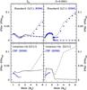 |
Fig. 3 Relative enrichment of the surface abundance of 4He with respect to its initial value (in mass fraction) for Paper I models at the end of the first and second dredge-up (solid and dashed black lines, respectively) as a function of the initial stellar mass and for two metallicities (Z⊙ and Z = 0.0001; left and right panels, respectively). Top panels: our standard predictions are compared with those of BS99 (blue circles; open and full at the end of the first and second dredge-up, respectively). Bottom panels: our models including both rotation-induced mixing and thermohaline instability are compared with the “cool-bottom processing” predictions by BS99 at the RGB tip (blue squares). |
2.3.2. Impact of rotation-induced mixing and thermohaline instability on model predictions
Thermohaline instability has no significant impact on the surface abundance of 4He since it develops only in the upper wing of the hydrogen-burning shell (see e.g. Paper I for more details)3. However, rotation-induced mixing smoothes the internal abundance gradients compared to the standard case, leading freshly produced 4He to diffuse outwards. This can be seen in Fig. 4 where we show the abundance profile of 4He at the end of the main sequence for two stellar masses and metallicities in the standard and the rotating cases (black full and red dashed lines, respectively; the vertical bars indicate the depth reached by the convective envelope at its maximum extent during the first dredge-up). This results in stronger 4He abundance variations at the end of the first dredge-up when rotation-induced mixing is accounted for, as seen in Fig. 3 (bottom panels). For the same reasons, the effect of the second dredge-up is also strengthened in the rotating models. Overall, the impact of rotation increases with decreasing metallicity (see Paper I, and references therein).
Consequently, the yields of 4He are higher in the models including rotation-induced mixing than in the standard case (see Tables 3 to 6). And at the same time, the fraction of H is decreased.
Figure 5 summarizes all the effects described above on the surface abundance of 4He along the evolution of standard and rotating stars with different initial masses at solar metallicity. The tracks are shown from the zero age main sequence up to the end of the TP-AGB, with the colour coding given on the right scale.
2.3.3. Comparison with other stellar models
In Fig. 3 we compare our predictions with those of Boothroyd & Sackmann (1999). We note a very good agreement as far as the standard models are concerned (upper panels). On the other hand, neither the thermohaline instability nor BS99 “cool bottom processing” do affect the 4He surface abundances. The differences that appear in the lower panels result essentially from the effects of rotation-induced mixing.
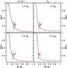 |
Fig. 4 Abundance profile of 4He at the end of the main sequence for the 1.5 M⊙ and 2.0 M⊙ models at two metallicities (Z = 0.0001 and Z = 0.014, left and right panel, respectively) in the standard case (solid black line), and when including the effects of rotation (red dashed line). Models are from Paper II. The maximum depth reached by the convective envelope during the first dredge-up is shown with the vertical bars and arrows. |
3. Chemical evolution model
3.1. Basic assumptions
The adopted model for the chemical evolution of the Galaxy assumes that the Milky Way forms out of two main accretion episodes almost completely disentangled (Chiappini et al. 1997, 2001). During the first one, the primordial gas collapses very quickly and forms the spheroidal components, halo and bulge. During the second one, the thin-disc forms, mainly by accretion of matter of primordial chemical composition. The disc is built-up in the framework of the inside-out scenario of Galaxy formation, which ensures the formation of abundance gradients along the disc (Larson 1976; Matteucci & Francois 1989). The Galactic disc is approximated by several independent rings, 2 kpc wide, without exchange of matter between them.
Description of different models computed with yields from Lagarde et al. (2011) for stars below 6 M⊙.
3.2. Nucleosynthesis prescriptions
The nucleosynthesis prescriptions for metals (elements heavier than 4He) are from Paper II for low- and intermediate-mass stars (M ≤ 6 M⊙). As for massive stars and Type Ia supernovae, we adopt the same nucleosynthesis prescriptions as in Romano et al. (2010), their model 6, namely:
-
yields for core-collapse supernovae are taken from Kobayashi et al. (2006), except for carbon, nitrogen and oxygen, for which the adopted yields are from Meynet & Maeder (2002); Hirschi et al. (2005); Hirschi (2007); Ekström et al. (2008);
-
yields for Type Ia supernovae are from Iwamoto et al. (1999).
-
In Model A we consider the standard yields for all stars with masses below 6.0 M⊙.
-
In Model B we consider the yields including thermohaline instability and rotation-induced mixing for 100% of the intermediate-mass stars (M > 2.5 M⊙) and 96% of the low-mass stars (M ≤ 2.5 M⊙). The remaining 4% of the low-mass stars are assumed to release the yields as predicted by the standard theory. This allows us to account for the fact that some rare planetary nebulae (J320, NGC 3242) exhibit 3He as predicted by the standard models (see e.g. Balser et al. 2007, and references therein).
-
In Model C we assume the yields including thermohaline instability and rotation-induced mixing for all the low- and intermediate-mass stars. Obviously the outcome of Models B and C are expected to be very similar.
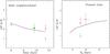 |
Fig. 6 Evolution of D/H in the solar neighborhood (left panel) and distribution of D/H along the Galactic disc at the present time (right panel). The predictions of Models A and B are shown (red solid and dashed blue lines, respectively). At t = 0 Gyr, we plot the WMAP value (filled black diamond). The PSC data by Geiss & Gloeckler (1998) are shown (filled green circle). The local interstellar medium (LISM) data are from Linsky et al. (2006), Hébrard et al. (2005) and Prodanović et al. (2010) (filled orange, light blue, and magenta triangles, respectively). The data for the outer disc (RG = 10 kpc) are from Rogers et al. (2005, filled bordeaux circle). |
4. Evolution of the light elements in the Milky Way
In the following sections we discuss the evolution of the light elements in the Galaxy within the framework described in Sect. 3 when taking into account the yields from our non-standard stellar models, and compare the predictions with different observations. The relevant data are presented in Table 1.
Model results for metallicity of Z = 0.0001.
4.1. Evolution of deuterium
In this paper we assume (D/H)P = 2.6 × 10⁻⁵ for consistency with the initial value adopted by the stellar models. However, we note that our GCE model gives a better fit to the data when a value of (D/H)P = 2.8 × 10⁻⁵ as observed in quasar spectra (Pettini et al. 2008) is adopted instead (see Fig. 3 of Romano 2010).
Figure 6 (left panel) shows the data for deuterium from the Big Bang (WMAP value, filled black diamond) to the present day (local interstellar medium, LISM, filled triangles). The determinations of primordial and PSC (filled green circle, Geiss & Gloeckler 1998, according with Geiss & Reeves 1972, 1981) deuterium abundances underline a small depletion from the Big Bang (t = 0 Gyr) to the solar-system formation (t = 9.2 Gyr). Analyses of Far Ultraviolet Spectroscopic Explorer (FUSE) observations have allowed measurements of D/H in the LISM for many lines of sight. These observations have revealed a large variation of the local D abundances, which complicates the interpretation in the context of standard GCE models (Linsky et al. 2006; Linsky 2010). Hébrard et al. (2005) and Linsky et al. (2006) proposed that either the lowest (D/H = 0.98 × 10⁻⁵) or the highest (D/H = 2.31 × 10⁻⁵) observed value is indicative of the true LISM value reflecting the process of D astration through successive stellar generations during the whole Galaxy’s evolution. Hébrard et al. (2005) suggest a value of the true local deuterium abundance lower than the one measured in the local bubble. On the other hand, Linsky et al. (2006) give a lower bound to the true local deuterium abundance very close to the primordial abundance, pointing to a deuterium astration factor smaller than predicted by standard GCE models. More recently, Prodanović et al. (2010) have applyed a statistical Bayesian method to determine the true local D abundance. They propose a value very close to the D abundance at the time of the formation of the Sun (see Table 1). GCE models that fulfil all the major observational constraints available for the solar neighbourhood and for the Milky Way disc can explain the LISM D abundance suggested by Prodanović et al. (2010) as a result of D astration during Galactic evolution; lower and higher values can only be explained as due to small-scale, transient phenomena, such as D depletion on to dust grains and localized infall of gas of primordial chemical composition (Romano et al. 2006; Steigman et al. 2007; Romano 2010, and references therein).
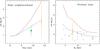 |
Fig. 7 Left panel: evolution of 3He/H with time in the solar neighborhood. Data for the PSC (green filled circle) and local interstellar medium (LISM, orange filled triangle) are from Geiss & Gloeckler (1998) and Gloeckler & Geiss (1996), respectively. 1-σ and 3-σ error bars are shown with thick and thin lines, respectively. Right panel: radial distribution of 3He/H at the present time. The dots are HII regions data from Bania et al. (2002) (error bars are shown only for S209; see text for discussion). The triangle at RG = 8 kpc represents LISM data from Gloeckler & Geiss (1996). The predictions from Models A, B and C are shown in both panels by the red full, blue dashed and cyan dotted lines respectively. |
Our predictions for the evolution of deuterium with time in the solar neighborhood and for the present deuterium abundance profile along the Milky Way disc are shown in Fig. 6 (left and right panels, respectively). The very modest shift between the predictions of Models A and B is due to the slight difference in the H yields when stellar rotation is accounted for compared to the standard case. Since pristine deuterium burns entirely in stars independently of their mass and metallicity, the predicted trends depend only on the total astration assumed in the GCE model. The present predictions fit well the PSC deuterium data and favour the local abundance of deuterium suggested by Prodanović et al. (2010).
4.2. Evolution of 3He
Figure 7 (left panel) shows the evolution of 3He/H in the solar neighborhood as predicted by Models A, B, and C (see Sect. 3.2). As already discussed in the literature (see Sect. 1), standard stellar models strongly overestimate the production of 3He by low-mass stars.
According to standard predictions, 3He is produced on the main sequence during the core hydrogen burning and it is not destroyed during later phases. Consequently, when adopting standard predictions 3He is overproduced in the course of Galactic evolution (Model A, red solid line). In low-mass stellar models including thermohaline mixing, 3He is destroyed from the bump luminosity on the RGB during shell hydrogen burning and during the early AGB. When low-mass stars are assumed to experience this extra-mixing, GCE models do not overproduce 3He (Fig. 7, Model C, cyan dotted line). Model B (dashed blue line) shows the effect of inhibiting the thermohaline mixing in 4% of low-mass stars (see Sect. 3.2), that thus follow the standard prescriptions. As can be seen in Fig. 7, negligible differences are found between Model B and Model C predictions. The PSC and local 3He abundances (Geiss & Gloeckler 1998; Gloeckler & Geiss 1996) are reproduced by the models (at 3- and 1-sigma level, respectively).
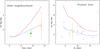 |
Fig. 8 Temporal (left panel) and spatial (right panel) variation of helium isotopic ratio in the solar neighborhood and along the galactic disk at the present time, respectively. Models are the same as in Fig. 7. Data are from Geiss & Gloeckler (1998) for the PSC (green filled circle), Bania et al. (2002) for Galactic HII regions (black dots), and Gloeckler & Geiss (1996) for the LISM (orange filled trangle). 1-σ and 3-σ errors are also shown as thick and thin lines, respectively. |
The present-day 3He abundance distribution along the Galactic disk is shown in Fig. 7 (right panel). Model A, adopting standard 3He yields for low-mass stars, predicts too much 3He at all Galactocentric distances. In the inner regions, where the star formation was stronger, the contribution of low- and intermediate-mass stars to the 3He enrichment of the ISM is more important. As a consequence, Model A predicts a large negative gradient of 3He/H. Although the contribution of low-mass stars in the inner regions is significantly reduced in Model B, it still predicts a negative gradient. In Fig. 7, we compare the predictions of Models A and B with observations of 3He in HII regions from Bania et al. (2002) and with the local 3He abundance from Gloeckler & Geiss (1996). Contrary to what is predicted by classical theory, the observations in HII regions show a gradient close to zero. Bania et al. (2002) derived meaningful error estimates only for one source [S209: 3He/H = (1.1 ± 0.2) × 10-5) and pointed our the riskiness of basing one’s conclusion on only one object. In order to better constrain both stellar and galactic evolution studies, it would be very useful if future work could provide a sound estimate of the errors associated to 3He determinations across the Galactic disk. Nevertheless, we can conclude that thermohaline and rotating mixing are required to fit currently available measurements of 3He in Galactic HII regions. In addition, the 3He gradient is d log(3He/H)/d RG ~ −0.04 and − 0.028 dex/kpc for Models A and B, respectively, consistent with that predicted by Chiappini et al. (2002), −0.04 < d log(3He/H)/d RG < −0.03 dex/kpc.
Tosi (2000) showed that GCE models including the CBP (Boothroyd & Sackmann 1999) also fit the relevant Galactic 3He data, provided the primordial abundance of D is sufficiently low (see also Chiappini et al. 2002; Romano et al. 2003). However, CBP destructs 3He too quickly and is not a physical mechanism (see Sect. 2.2). Therefore, it does not provide a reliable physical explanation of the 3He observations in HII regions.
4.3. Evolution of 4He
Figure 8 shows the temporal (left panel) and the spatial (right panel) evolution of the helium isotopic ratio (3He/4He) in the solar neighborhood and along the Galactic disk at the present time, respectively. Only the predictions of Models A and B are shown in the right panel. The PSC and LISM data are from Geiss & Gloeckler (1998) and Gloeckler & Geiss (1996), respectively. The standard theory predicts a significant evolution of the helium isotopic ratio in the Galaxy, and a strong gradient across the Galactic disc. When the thermohaline mixing – which destroys 3He in the stellar interior – and the rotation-induced mixing – which increases 4He at the stellar surface (see Sect. 3.3) – are taken into account, lower helium isotopic ratios are obtained (cf. the dashed versus solid lines in Fig. 8). Consequently, the gradient of the helium isotopic ratio across the Galactic disc decreases and the observations in HII regions can be reproduced.
Figure 9 presents the predictions for Y versus [Fe/H] in the solar neighborhood. The model predictions are compared with the initial abundance of 4He in the Sun derived by Serenelli (2010) from full standard solar models computed for different sets of solar abundances. When the solar abundances from Grevesse & Sauval (1998) and a metal to hydrogen ratio in the solar photosphere of (Z / X)ph = 0.0229 are adopted, a value of Yi = 0.2721 is obtained, which results in good agreement with the predictions of chemical evolution models including rotation-induced mixing and thermohaline mixing (green Sun symbol and dashed and dotted lines in Fig. 9, respectively). On the other hand, choosing the solar abundances from Asplund et al. (2009) and (Z / X)ph = 0.0178 result in Yi = 0.2653, which is better fitted by models including standard stellar nucleosynthesis (orange Sun symbol and solid line in Fig. 9). Since the actual solar chemical composition is matter of debate, we can not discriminate between our models basing on the results for Y.
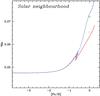 |
Fig. 9 Y versus [Fe/H] in the solar neighborhood predicted by models including yields computed with standard prescriptions (Model A; solid line) and with thermohaline mixing and rotation-induced mixing (Models B and C; dashed and dotted lines, respectively). Model predictions are compared with the protosolar values given by Serenelli (2010). |
5. Conclusions
In this article, we have described the results for the Galactic evolution of the primordial elements D, 3He and 4He in the light of new stellar models including the effects of thermohaline instability and rotation-induced mixing on the stellar structure, evolution and nucleosynthesis. The new stellar models are presented and discussed at length in Charbonnel & Lagarde (2010) and Lagarde et al. (2011). We model the time-behavior of D, 3He and 4He in the solar neighbourhood, as well as in the inner and outer disc. The predictions of our models including thermohaline instability and rotation-induced mixing are compared to the predictions of models adopting standard nucleosynthesis prescriptions and to the most recent relevant observations.
We have seen that the CBP proposed before by Boothroyd & Sackmann (1999) is not a physical mechanism, and yields deduced do not take into account phases beyond the RGB. As discussed in the literature (Charbonnel & Zahn 2007b; Charbonnel & Lagarde 2010; Lagarde et al. 2011), thermohaline mixing can induces significant depletion of 3He in low- and intermediate-mass stars. Although these stars remain net producers of 3He, their contribution to the Galactic evolution of this element is highly reduced compared to classical theory. Indeed, our GCE models including thermohaline mixing reproduce the observations of 3He in the PSC, LISM and HII regions, while 3He is overproduced on a Galactic scale with standard models. Thermohaline mixing is the only physical mechanism known so far able to solve the so-called “3He problem” plaguing in the literature since many years. Importantly, its inhibition by a fossil magnetic field in red giant stars that are descendants of Ap stars does reconcile the measurements of 3He/H in Galactic HII regions with high values of 3He in a couple of planetary nebulae.
On the other hand, rotation has an impact on the stellar yields of H and 4He. Whether GCE models including rotation fit better the Galactic 4He data than standard models can not be said, because of the uncertainties on the actual solar chemical composition. However, they are consistent with the relatively high value of (D/H)LISM proposed by Prodanović et al. (2010).
We conclude that GCE models including both thermohaline mixing and rotation-induced mixing reproduce satisfactorily well all the available data on D, 3He and, possibly, 4He abundances in the Milky Way, within the errors. However, the additional data on HII regions and better refining of their interpolation would be crucial to assess how good our fit actually is.
To translate the thermohaline diffusion coefficient of our models into a stream mass flow rate as used by BS99, we compute:
 with r and ρ the radius and the density at the base of the region where the thermohaline instability develops, lmix the size of this mixing zone, and
  the mean diffusion coefficient along the mixing zone.
Note that we did not include additional mechanisms to force the third dredge-up in our models, as required in the literature for reproducing the carbon-star luminosity function (e.g. Frogel et al. 1990; Costa & Frogel 1996; Groenewegen 1998; Marigo et al. 1999). Hence, we do not attempt any comparison of the model predictions with available data for C and N isotopes. However this has no impact on the galactic chemical evolution of the light elements we focus on.
Thermohaline mixing leads to an increase of the surface abundance of 4He during the RGB by ~0.1% in the 1.25 M⊙ models independently of the stellar metallicity.
Acknowledgments
We dedicate this paper to Robert T. Rood: the scientist to whom the stellar evolution and 3He communities owe so much, and the friend whom we will miss for ever. We thank T. Bania, D. Balser, and H. Reeves for fruitful discussions. We are thankful to our referee, Dr Achim Weiss, for his interesting and constructive remarks on our article. C.C., D.R., and M.T. gratefully acknowledge the enlightening and fascinating conversations with Johannes Geiss and his hospitality at the International Space Science Institute (ISSI) in Bern (CH). We acknowledge financial support from the Swiss National Science Foundation (FNS) and the french Programme National de Physique Stellaire (PNPS) of CNRS/INSU.
References
- Asplund, M., Grevesse, N., Sauval, A. J., & Scott, P. 2009, ARA&A, 47, 481 [NASA ADS] [CrossRef] [Google Scholar]
- Balser, D. S., Bania, T. M., Rood, R. T., & Wilson, T. L. 1999, ApJ, 510, 759 [NASA ADS] [CrossRef] [Google Scholar]
- Balser, D. S., Goss, W. M., Bania, T. M., & Rood, R. T. 2006, ApJ, 640, 360 [NASA ADS] [CrossRef] [Google Scholar]
- Balser, D. S., Rood, R. T., & Bania, T. M. 2007, Science, 317, 1171 [NASA ADS] [CrossRef] [PubMed] [Google Scholar]
- Balser, D., Rood, T. R., & Bania, T. M. 2010, in IAU Symp. 268, ed. C. Charbonnel, M. Tosi, F. Primas, & C. Chiappini, 101 [Google Scholar]
- Bania, T. M., Rood, R. T., & Balser, D. S. 2002, Nature, 415, 54 [NASA ADS] [CrossRef] [PubMed] [Google Scholar]
- Bania, T. M., Rood, R. T., & Balser, D. S. 2010, in IAU Symp. 268, ed. C. Charbonnel, M. Tosi, F. Primas, & C. Chiappini, 81 [Google Scholar]
- Bennett, C. L., Halpern, M., Hinshaw, G., et al. 2003, ApJS, 148, 1 [NASA ADS] [CrossRef] [Google Scholar]
- Boothroyd, A. I., & Sackmann, I.-J. 1999, ApJ, 510, 232 [Google Scholar]
- Burles, S., & Tytler, D. 1998, ApJ, 507, 732 [NASA ADS] [CrossRef] [Google Scholar]
- Charbonnel, C. 1995, ApJ, 453, L41 [NASA ADS] [CrossRef] [Google Scholar]
- Charbonnel, C., & Do Nascimento, Jr., J. D. 1998, A&A, 336, 915 [NASA ADS] [Google Scholar]
- Charbonnel, C., & Lagarde, N. 2010, A&A, 522, A10 [NASA ADS] [CrossRef] [EDP Sciences] [MathSciNet] [PubMed] [Google Scholar]
- Charbonnel, C., & Zahn, J. 2007a, A&A, 476, L29 [NASA ADS] [CrossRef] [EDP Sciences] [Google Scholar]
- Charbonnel, C., & Zahn, J.-P. 2007b, A&A, 467, L15 [NASA ADS] [CrossRef] [EDP Sciences] [Google Scholar]
- Chiappini, C., Matteucci, F., & Gratton, R. 1997, ApJ, 477, 765 [NASA ADS] [CrossRef] [Google Scholar]
- Chiappini, C., Matteucci, F., & Romano, D. 2001, ApJ, 554, 1044 [NASA ADS] [CrossRef] [Google Scholar]
- Chiappini, C., Renda, A., & Matteucci, F. 2002, A&A, 395, 789 [NASA ADS] [CrossRef] [EDP Sciences] [Google Scholar]
- Coc, A., Vangioni-Flam, E., Descouvemont, P., Adahchour, A., & Angulo, C. 2004, ApJ, 600, 544 [NASA ADS] [CrossRef] [Google Scholar]
- Costa, E., & Frogel, J. A. 1996, AJ, 112, 2607 [NASA ADS] [CrossRef] [Google Scholar]
- Cyburt, R. H., Fields, B. D., & Olive, K. A. 2008, J. Cosmology Astropart. Phys., 11, 12 [Google Scholar]
- Dearborn, D. S. P., Steigman, G., & Tosi, M. 1996, ApJ, 465, 887 [NASA ADS] [CrossRef] [Google Scholar]
- Denissenkov, P. A. 2010, ApJ, 723, 563 [NASA ADS] [CrossRef] [Google Scholar]
- Denissenkov, P. A., & Merryfield, W. J. 2011, ApJ, 727, L8 [NASA ADS] [CrossRef] [Google Scholar]
- Edmunds, M. G. 1994, MNRAS, 270, L37 [NASA ADS] [Google Scholar]
- Eggleton, P. P., Dearborn, D. S. P., & Lattanzio, J. C. 2006, Science, 314, 1580 [NASA ADS] [CrossRef] [PubMed] [Google Scholar]
- Eggleton, P. P., Dearborn, D. S. P., & Lattanzio, J. C. 2008, ApJ, 677, 581 [NASA ADS] [CrossRef] [Google Scholar]
- Ekström, S., Meynet, G., Chiappini, C., Hirschi, R., & Maeder, A. 2008, A&A, 489, 685 [NASA ADS] [CrossRef] [EDP Sciences] [Google Scholar]
- Epstein, R. I., Lattimer, J. M., & Schramm, D. N. 1976, Nature, 263, 198 [NASA ADS] [CrossRef] [Google Scholar]
- Frogel, J. A., Mould, J., & Blanco, V. M. 1990, ApJ, 352, 96 [NASA ADS] [CrossRef] [Google Scholar]
- Galli, D., Palla, F., Ferrini, F., & Penco, U. 1995, ApJ, 443, 536 [NASA ADS] [CrossRef] [Google Scholar]
- Galli, D., Stanghellini, L., Tosi, M., & Palla, F. 1997, ApJ, 477, 218 [NASA ADS] [CrossRef] [Google Scholar]
- Geiss, J., & Gloeckler, G. 1998, Space Sci. Rev., 84, 239 [NASA ADS] [CrossRef] [Google Scholar]
- Geiss, J., & Reeves, H. 1972, A&A, 18, 126 [NASA ADS] [Google Scholar]
- Geiss, J., & Reeves, H. 1981, A&A, 93, 189 [Google Scholar]
- Gloeckler, G., & Geiss, J. 1996, Nature, 381, 210 [NASA ADS] [CrossRef] [Google Scholar]
- Grevesse, N., & Sauval, A. J. 1998, Space Sci. Rev., 85, 161 [NASA ADS] [CrossRef] [Google Scholar]
- Groenewegen, M. A. T. 1998, Ap&SS, 255, 379 [Google Scholar]
- Hébrard, G., Lemoine, M., Vidal-Madjar, A., et al. 2002, ApJS, 140, 103 [NASA ADS] [CrossRef] [Google Scholar]
- Hébrard, G., Tripp, T. M., Chayer, P., et al. 2005, ApJ, 635, 1136 [NASA ADS] [CrossRef] [Google Scholar]
- Hirschi, R. 2007, A&A, 461, 571 [NASA ADS] [CrossRef] [EDP Sciences] [Google Scholar]
- Hirschi, R., Meynet, G., & Maeder, A. 2005, A&A, 433, 1013 [NASA ADS] [CrossRef] [EDP Sciences] [Google Scholar]
- Hogan, C. J. 1995, ApJ, 441, L17 [NASA ADS] [CrossRef] [Google Scholar]
- Iben, Jr., I. 1967, ApJ, 147, 624 [NASA ADS] [CrossRef] [Google Scholar]
- Iwamoto, K., Brachwitz, F., Nomoto, K., et al. 1999, ApJS, 125, 439 [NASA ADS] [CrossRef] [MathSciNet] [Google Scholar]
- Jenkins, E. B., Tripp, T. M., Woźniak, P. R., Sofia, U. J., & Sonneborn, G. 1999, ApJ, 520, 182 [NASA ADS] [CrossRef] [Google Scholar]
- Kobayashi, C., Umeda, H., Nomoto, K., Tominaga, N., & Ohkubo, T. 2006, ApJ, 653, 1145 [NASA ADS] [CrossRef] [Google Scholar]
- Krishnamurti, R. 2003, J. Fluid Mech., 483, 287 [NASA ADS] [CrossRef] [Google Scholar]
- Lagarde, N., Charbonnel, C., Decressin, T., & Hagelberg, J. 2011, A&A, 536, A28 [NASA ADS] [CrossRef] [EDP Sciences] [Google Scholar]
- Lagarde, N., Decressin, T., Charbonnel, C., et al. 2012, A&A, in press, DOI:10.1051/0004-6361/201118331 [Google Scholar]
- Larson, R. B. 1976, MNRAS, 176, 31 [NASA ADS] [CrossRef] [Google Scholar]
- Linsky, J. L. 2010, in IAU Symp. 268, ed. C. Charbonnel, M. Tosi, F. Primas, & C. Chiappini, 53 [Google Scholar]
- Linsky, J. L., Draine, B. T., Moos, H. W., et al. 2006, ApJ, 647, 1106 [NASA ADS] [CrossRef] [Google Scholar]
- Maeder, A., & Zahn, J.-P. 1998, A&A, 334, 1000 [NASA ADS] [Google Scholar]
- Marigo, P., Girardi, L., & Bressan, A. 1999, A&A, 344, 123 [NASA ADS] [Google Scholar]
- Matteucci, F., & Francois, P. 1989, MNRAS, 239, 885 [NASA ADS] [CrossRef] [Google Scholar]
- Meynet, G., & Maeder, A. 2002, A&A, 390, 561 [NASA ADS] [CrossRef] [EDP Sciences] [Google Scholar]
- Oliveira, C. M., & Hébrard, G. 2006, ApJ, 653, 345 [NASA ADS] [CrossRef] [Google Scholar]
- Palla, F., Bachiller, R., Stanghellini, L., Tosi, M., & Galli, D. 2000, A&A, 355, 69 [NASA ADS] [Google Scholar]
- Peebles, P. J. E. 1966, ApJ, 146, 542 [NASA ADS] [CrossRef] [Google Scholar]
- Peimbert, M., Peimbert, A., Carigi, L., & Luridiana, V. 2010, in IAU Symp. 268, ed. C. Charbonnel, M. Tosi, F. Primas, & C. Chiappini, 91 [Google Scholar]
- Pettini, M., Zych, B. J., Murphy, M. T., Lewis, A., & Steidel, C. C. 2008, MNRAS, 391, 1499 [NASA ADS] [CrossRef] [MathSciNet] [Google Scholar]
- Prantzos, N. 1996, A&A, 310, 106 [NASA ADS] [Google Scholar]
- Prodanović, T., & Fields, B. D. 2003, ApJ, 597, 48 [NASA ADS] [CrossRef] [Google Scholar]
- Prodanović, T., Steigman, G., & Fields, B. D. 2010, MNRAS, 406, 1108 [NASA ADS] [Google Scholar]
- Reeves, H., Audouze, J., Fowler, W. A., & Schramm, D. N. 1973, ApJ, 179, 909 [NASA ADS] [CrossRef] [Google Scholar]
- Rogers, A. E. E., Dudevoir, K. A., Carter, J. C., et al. 2005, ApJ, 630, L41 [NASA ADS] [CrossRef] [Google Scholar]
- Romano, D. 2010, in IAU Symp. 268, ed. C. Charbonnel, M. Tosi, F. Primas, & C. Chiappini, 431 [Google Scholar]
- Romano, D., Tosi, M., Matteucci, F., & Chiappini, C. 2003, MNRAS, 346, 295 [NASA ADS] [CrossRef] [Google Scholar]
- Romano, D., Tosi, M., Chiappini, C., & Matteucci, F. 2006, MNRAS, 369, 295 [NASA ADS] [CrossRef] [Google Scholar]
- Romano, D., Karakas, A. I., Tosi, M., & Matteucci, F. 2010, A&A, 522, A32 [NASA ADS] [CrossRef] [EDP Sciences] [Google Scholar]
- Rood, R. T., Steigman, G., & Tinsley, B. M. 1976, ApJ, 207, L57 [NASA ADS] [CrossRef] [Google Scholar]
- Rood, R. T., Bania, T. M., & Wilson, T. L. 1984, ApJ, 280, 629 [NASA ADS] [CrossRef] [Google Scholar]
- Rood, R. T., Bania, T. M., & Wilson, T. L. 1992, Nature, 355, 618 [NASA ADS] [CrossRef] [Google Scholar]
- Rosenblum, E., Garaud, P., Traxler, A., & Stellmach, S. 2011, ApJ, 731, 66 [NASA ADS] [CrossRef] [Google Scholar]
- Serenelli, A. M. 2010, Ap&SS, 328, 13 [NASA ADS] [CrossRef] [Google Scholar]
- Songaila, A., Cowie, L. L., Hogan, C. J., & Rugers, M. 1994, Nature, 368, 599 [NASA ADS] [CrossRef] [Google Scholar]
- Sonneborn, G., Tripp, T. M., Ferlet, R., et al. 2000, ApJ, 545, 277 [NASA ADS] [CrossRef] [Google Scholar]
- Spergel, D. N., Verde, L., Peiris, H. V., et al. 2003, ApJS, 148, 175 [NASA ADS] [CrossRef] [Google Scholar]
- Steigman, G., & Tosi, M. 1992, ApJ, 401, 150 [NASA ADS] [CrossRef] [Google Scholar]
- Steigman, G., Romano, D., & Tosi, M. 2007, MNRAS, 378, 576 [NASA ADS] [CrossRef] [Google Scholar]
- Tosi, M. 2000, in The Light Elements and their Evolution, ed. L. da Silva, R. de Medeiros, & M. Spite, IAU Symp., 198, 525 [Google Scholar]
- Tosi, M., Steigman, G., Matteucci, F., & Chiappini, C. 1998, ApJ, 498, 226 [NASA ADS] [CrossRef] [Google Scholar]
- Traxler, A., Garaud, P., & Stellmach, S. 2011, ApJ, 728, L29 [NASA ADS] [CrossRef] [Google Scholar]
- Truran, J. W., & Cameron, A. G. W. 1971, Ap&SS, 14, 179 [NASA ADS] [CrossRef] [Google Scholar]
- Ulrich, R. K. 1972, ApJ, 172, 165 [NASA ADS] [CrossRef] [Google Scholar]
- Vidal-Madjar, A., Lemoine, M., Ferlet, R., et al. 1998, A&A, 338, 694 [NASA ADS] [Google Scholar]
- Wagoner, R. V., Fowler, W. A., & Hoyle, F. 1967, ApJ, 148, 3 [NASA ADS] [CrossRef] [Google Scholar]
- Weiss, A., Wagenhuber, J., & Denissenkov, P. A. 1996, A&A, 313, 581 [NASA ADS] [Google Scholar]
- Zahn, J.-P. 1992, A&A, 265, 115 [NASA ADS] [Google Scholar]
All Tables
Description of different models computed with yields from Lagarde et al. (2011) for stars below 6 M⊙.
All Figures
|
Fig. 1 Theoretical evolutionary tracks in the HR diagram for the 1.5 M⊙, 3.0 M⊙, and 6.0 M⊙ models at solar metallicity following the standard prescription (left panel); and including rotation-induced mixing and thermohaline instability (right panel), from the pre-main sequence up to the end of the TP-AGB phase. Colours depict the mass fraction of 3He at the stellar surface as indicated on the right, with the arrows showing the initial 3He and 3He + 2H content assumed at birth. |
| In the text | |
|
Fig. 2 Mass fraction of 3He at the stellar surface at the end of the second dredge-up as a function of initial stellar mass in standard models (solid lines and triangles) and in models including various prescriptions for mixing in the radiative regions (dashed lines), at two metallicities (Z = 0.0001 and Z = 0.014; left and right panels, respectively). The predictions are from Dearborn et al. (1996, DST96, blue line), Boothroyd & Sackmann (1999, BS99, at the RGB tip, magenta lines), Weiss et al. (1996, WWD96, red triangles), and Lagarde et al. (2011, LC11, black lines). The initial abundances of 3He adopted at the zero age main sequence by the different authors are given on the top right corner of each panel. |
| In the text | |
|
Fig. 3 Relative enrichment of the surface abundance of 4He with respect to its initial value (in mass fraction) for Paper I models at the end of the first and second dredge-up (solid and dashed black lines, respectively) as a function of the initial stellar mass and for two metallicities (Z⊙ and Z = 0.0001; left and right panels, respectively). Top panels: our standard predictions are compared with those of BS99 (blue circles; open and full at the end of the first and second dredge-up, respectively). Bottom panels: our models including both rotation-induced mixing and thermohaline instability are compared with the “cool-bottom processing” predictions by BS99 at the RGB tip (blue squares). |
| In the text | |
|
Fig. 4 Abundance profile of 4He at the end of the main sequence for the 1.5 M⊙ and 2.0 M⊙ models at two metallicities (Z = 0.0001 and Z = 0.014, left and right panel, respectively) in the standard case (solid black line), and when including the effects of rotation (red dashed line). Models are from Paper II. The maximum depth reached by the convective envelope during the first dredge-up is shown with the vertical bars and arrows. |
| In the text | |
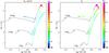 |
Fig. 5 Same as Fig. 1 for 4He from the zero age main sequence to the end of the TP-AGB. |
| In the text | |
|
Fig. 6 Evolution of D/H in the solar neighborhood (left panel) and distribution of D/H along the Galactic disc at the present time (right panel). The predictions of Models A and B are shown (red solid and dashed blue lines, respectively). At t = 0 Gyr, we plot the WMAP value (filled black diamond). The PSC data by Geiss & Gloeckler (1998) are shown (filled green circle). The local interstellar medium (LISM) data are from Linsky et al. (2006), Hébrard et al. (2005) and Prodanović et al. (2010) (filled orange, light blue, and magenta triangles, respectively). The data for the outer disc (RG = 10 kpc) are from Rogers et al. (2005, filled bordeaux circle). |
| In the text | |
|
Fig. 7 Left panel: evolution of 3He/H with time in the solar neighborhood. Data for the PSC (green filled circle) and local interstellar medium (LISM, orange filled triangle) are from Geiss & Gloeckler (1998) and Gloeckler & Geiss (1996), respectively. 1-σ and 3-σ error bars are shown with thick and thin lines, respectively. Right panel: radial distribution of 3He/H at the present time. The dots are HII regions data from Bania et al. (2002) (error bars are shown only for S209; see text for discussion). The triangle at RG = 8 kpc represents LISM data from Gloeckler & Geiss (1996). The predictions from Models A, B and C are shown in both panels by the red full, blue dashed and cyan dotted lines respectively. |
| In the text | |
|
Fig. 8 Temporal (left panel) and spatial (right panel) variation of helium isotopic ratio in the solar neighborhood and along the galactic disk at the present time, respectively. Models are the same as in Fig. 7. Data are from Geiss & Gloeckler (1998) for the PSC (green filled circle), Bania et al. (2002) for Galactic HII regions (black dots), and Gloeckler & Geiss (1996) for the LISM (orange filled trangle). 1-σ and 3-σ errors are also shown as thick and thin lines, respectively. |
| In the text | |
|
Fig. 9 Y versus [Fe/H] in the solar neighborhood predicted by models including yields computed with standard prescriptions (Model A; solid line) and with thermohaline mixing and rotation-induced mixing (Models B and C; dashed and dotted lines, respectively). Model predictions are compared with the protosolar values given by Serenelli (2010). |
| In the text | |
Current usage metrics show cumulative count of Article Views (full-text article views including HTML views, PDF and ePub downloads, according to the available data) and Abstracts Views on Vision4Press platform.
Data correspond to usage on the plateform after 2015. The current usage metrics is available 48-96 hours after online publication and is updated daily on week days.
Initial download of the metrics may take a while.