| Issue |
A&A
Volume 542, June 2012
|
|
|---|---|---|
| Article Number | A51 | |
| Number of page(s) | 13 | |
| Section | Galactic structure, stellar clusters and populations | |
| DOI | https://doi.org/10.1051/0004-6361/201118744 | |
| Published online | 05 June 2012 | |
A primordial star in the heart of the Lion⋆
1 Zentrum für Astronomie der Universität Heidelberg, Landessternwarte, Königstuhl 12, 69117 Heidelberg, Germany
2 GEPI, Observatoire de Paris, CNRS, Univ. Paris Diderot, Place Jules Janssen, 92190 Meudon, France
e-mail: This email address is being protected from spambots. You need JavaScript enabled to view it.
3 European Southern Observatory, 19001 Casilla, Santiago, Chile
4 UPJV, Université de Picardie Jules Verne, 33 rue St Leu, 80080 Amiens, France
5 Istituto Nazionale di Astrofisica, Osservatorio Astronomico di Padova, Vicolo dell’Osservatorio 5, 35122 Padova, Italy
6 Leibniz-Institut für Astrophysik Potsdam, An der Sternwarte 16, 14482 Potsdam, Germany
7 Institute of Astronomy, Russian Academy of Sciences, 119017 Moscow, Russia
8 Istituto Nazionale di Astrofisica, Osservatorio Astronomico di Trieste, via Tiepolo 11, 34143 Trieste, Italy
9 Laboratoire Univers et Particules de Montpellier, LUPM, Université Montpellier 2, CNRS, 34095 Montpellier Cedex 5, France
10 Université de Nice Sophia Antipolis, CNRS, Observatoire de la Côte d’Azur, Laboratoire Cassiopée, BP 4229, 06304 Nice Cedex 4, France
11 Istituto Nazionale di Astrofisica, Osservatorio Astrofisico di Arcetri, Largo E. Fermi 5, 50125 Firenze, Italy
Received: 26 December 2011
Accepted: 2 March 2012
Abstract
Context. The discovery and chemical analysis of extremely metal-poor stars permit a better understanding of the star formation of the first generation of stars and of the Universe emerging from the Big Bang.
Aims. We report the study of a primordial star situated in the centre of the constellation Leo (SDSS J102915+172927).
Methods. The star, selected from the low-resolution spectrum of the Sloan Digital Sky Survey, was observed at intermediate (with X-Shooter at VLT) and at high spectral resolution (with UVES at VLT). The stellar parameters were derived from the photometry. The standard spectroscopic analysis based on 1D ATLAS models was completed by applying 3D and non-LTE corrections.
Results. An iron abundance of [Fe/H ] = −4.89 makes SDSS J102915+172927 one of the lowest [Fe/H] stars known. However, the absence of measurable C and N enhancements indicates that it has the lowest metallicity, Z ≤ 7.40 × 10⁻⁷ (metal-mass fraction), ever detected. No oxygen measurement was possible.
Conclusions. The discovery of SDSS J102915+172927 highlights that low-mass star formation occurred at metallicities lower than previously assumed. Even lower metallicity stars may yet be discovered, with a chemical composition closer to the composition of the primordial gas and of the first supernovae.
Key words: stars: abundances / stars: Population II / stars: Population III / stars: formation / Galaxy: evolution / cosmology: observations
Based on observations obtained at ESO Paranal Observatory, GTO programme 086.D-0094 and programme 286.D-5045.
Gliese Fellow.
© ESO, 2012
1. Introduction
Very metal-poor stars are the relic of the primordial Universe. They are formed from material whose composition is close to that of the Universe emerging from the Big Bang, only with traces of elements heavier than lithium, which were processed by the first generations of stars. A low-mass star (M < 0.8 M⊙) formed just after the Big Bang would still shine today on the main sequence, and could be easily recognised from its observed spectrum because only lines of hydrogen and the Li doublet at 670.7 nm would be visible. Such stars have not been detected, and some models of star formation state that it is impossible that such star might form. Indeed, it has been speculated that the first generation of stars consisted of massive stars (M > 80 M⊙Ostriker & Gnedin 1996) that evolved rapidly and synthetised metals that were ejected into space for the following generations of stars through a supernova type II explosion. This scenario is supported by the fact that no zero-metal star has been observed so far. But absence of evidence is not evidence of absence. Such stars, if they exist, could be very rare and faint. Some theories of star formation predict that the stars that formed from the ejecta of the first few generations of primordial massive stars needed a chemical pattern different from the one well-known in metal-poor stars that, apart from an enhancement in α-elements, have a scaled solar composition (Bonifacio et al. 2009). According to Bromm & Loeb (2003) and Schneider et al. (2003), a minimum metallicity is necessary to permit the cooling of the collapsing cloud for small-mass stars to form. In particular, according to Bromm & Loeb (2003), extremely iron-poor stars can form at sub-solar masses when enhanced in C and O. The discovery of some hyper-iron-poor and very carbon- and nitrogen-enhanced stars in the past decade (Christlieb et al. 2002; Frebel et al. 2005; Norris et al. 2007) supported the theory of Bromm & Loeb (2003). It is interesting to note that the cooling by dust (Omukai et al. 2008; Schneider et al. 2012) may imply a considerably lower critical metallicity, with no specific requirement of chemical composition. Another fundamental ingredient of star formation besides cooling is fragmentation. If a large-mass cloud can fragment into smaller pieces, then these pieces can form low-mass stars even in the absence of metals, the main cooling agent being molecular hydrogen (Nakamura & Umemura 2001). Recently, Clark et al. (2011) have shown that the first generation of stars are indeed likely to form as binary or multiple systems resulting from the fragmentation of an initial cloud of large mass. Under these conditions, Greif et al. (2011) derived an initial mass function (IMF) that is essentially flat between 0.1 and 10 solar masses. This IMF is top-heavy, in the sense that most of the mass is concentrated in a few massive stars, and yet it allows for the formation of low-mass stars. In this latter scenario there is no critical metallicity.
We present here the analysis of SDSS J102915+172927, an extremely metal-poor star, that shows no strong enhancement in carbon and nitrogen, and has a global metallicity more than four orders of magnitude lower than the solar one: Z ≤ 7.40 × 10⁻⁷, to be compared to Z⊙ = 1.53 × 10⁻² (Caffau et al. 2011a), giving a metallicity in respect with solar one of Z = 5 × 10⁻⁵ Z⊙. If CNO abundances are non-enhanced, Z = 7.15 × 10⁻⁷. With respect to the results presented earlier by our group (Caffau et al. 2011c), the present analysis uses of a custom CO5BOLD hydrodynamical model and NLTE computations for Mg, Si, Ca, Fe, and Sr.
2. Observations and data reduction
For SDSS J102915+172927 we availed ourselves of X-Shooter (D’Odorico et al. 2006) and UVES (Dekker et al. 2000) observations. The star was observed during the X-Shooter French-Italian Guaranteed Time of Observation (GTO) on 10 February 2011, programme 086.D-0094, P.I. P. Bonifacio. The spectral range covered is 330–2400 nm, split into three spectral arms (UVB, VIS, and NIR). For the integral field unit (IFU), which re-images an input field of 4′′ × 1.8′′ into a pseudo slit of 12′′ × 0.6′′ and a 1 × 2 binning, staring mode was used. Using the IFU as a slicer, the resolving power was R = 7900 in the UVB arm and R = 12 600 in the VIS arm. The spectra were reduced using the X-Shooter pipeline (Goldoni et al. 2006). The details on X-Shooter observations can be found in Caffau et al. (2011b).
On the basis of the highly promising analysis of the X-Shooter spectrum we applied for ESO Director Discretionary Time (DDT) to observe the star with UVES@VLT, and the observing blocks (OB) were observed on March-April 2011, within the programme 286.D-5045, P.I. P. Bonifacio. Five OBs were executed in DIC #1, standard 390 nm + 580 nm setting, two in DIC #2, standard 473 nm + 760 nm setting. All exposures had a length of 3000 s, slit width was set to 1.4′′, which led to an expected resolution of ~38 000. However, during most exposures the seeing was better than 1.4′′, thus leading to slightly better resolution in the final spectra. The signal-to-noise ratio per pixel at 650 nm was between 30 and 40 for all spectra.
Characteristics of the star SDSS J102915+172927.
3. Model atmospheres
The analysis was mainly performed with 1D plane-parallel hydrostatic model atmospheres, computed with ATLAS 9 (Kurucz 1993, 2005) in its Linux version (Sbordone et al. 2004; Sbordone 2005). The line opacity was treated through opacity distribution functions (ODFs), and we used the ODFs computed by Castelli & Kurucz (2004) for a scaled solar metallicity corresponding to [Fe/H ] = −4.5. The ATLAS 9 model was computed with the stellar parameters derived from photometry, as given in Table 1. The 3D abundance corrections were derived with a 3D-CO5BOLD model expressly computed for this star and the related 1DLHD model, computed with the LHD code (for details concerning the 3D corrections see Caffau et al. 2011a). To derive the 3D corrections on the chemical abundances we compared the abundance derived by using the 3D-CO5BOLD model with the abundance derived with 1D plane-parallel model, the 1DLHD model. The 1DLHD model employs the same micro-physics and radiative transfer scheme as the 3D-CO5BOLD model, so that any difference in the abundance determination is due to the 3D versus 1D treatment of convection. The 3D model used in the following was computed for stellar parameters Teff = 5850 K, log g = 4.0, [Fe/H] = −4.0. The computational domain is a cartesian box of size 25.8 × 25.8 × 12.5 Mm3, resolved by 200 × 200 × 200 cells. The frequency dependence of the total radiative opacity was approximately taken into account by adopting the opacity binning method (see e.g. Freytag et al. 2012), using a total of 11 frequency groups. The detailed monochromatic (continuous plus line) opacities needed to evaluate the average opacity for each frequency group as a function of P and T were derived from the MARCS stellar atmosphere package (Gustafsson et al. 2003, 2008) for metallicity [Fe/H ] = −4, [α/H] = 0.4 (Plez, priv. comm.).
The present 3D model differs from the one previously used for the calculation of 3D abundance corrections in Caffau et al. (2011c) in several aspects: (i) its metallicity is lower by a factor of 10 ([Fe/H] = −4 instead of −3); (ii) it uses a better frequency resolution (11 instead of 6 frequency groups); (iii) it has a higher spatial resolution (200 × 200 × 200 instead of 140 × 140 × 150 grid cells). Nevertheless, the mean temperature stratifications are quite similar (see Fig. 1), except for the upper photosphere (log τRoss < −3) where – contrary to expectations – the lower metallicity model shows somewhat higher temperatures. Both 3D models agree in the amplitude of the photospheric temperature fluctuations, which is fairly low, presumably because of H2 molecule formation in the higher photosphere. The most striking difference between the 3D and the 1D models is the temperature in the outer photosphere, which in both 3D models is significantly cooler than their 1DLHD counterparts.
The total 3D LTE abundance corrections (A(3D) – A(1DLHD)) were computed for all atomic lines measured in the observed spectra, assuming αMLT = 0.5, and a microturbulence parameter ξ = 1.5 km s-1 for the 1DLHD models. For the molecular bands, G-band and NH-band, representative lines were considered. Obviously, the physical reason for the large negative 3D corrections for Fe i and Ni i is the large 3D-1D temperature difference in the upper photosphere.
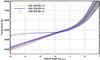 |
Fig. 1 Mean temperature structure as a function of Rosseland optical depth of the CO5BOLD model used in this work (Teff = 5850 K, log g = 4.0, [Fe/H ] = −4.0; thick [blue] line), and of the 3D model used in Caffau et al. (2011c) (5850/4.0/ − 3.0; thin [red] line). For each model, the mean temperature is obtained by averaging the temperature as |
![Mathematical equation: \hbox{$\sqrt[4]{\langle{T^4}\rangle}$}](/articles/aa/full_html/2012/06/aa18744-11/aa18744-11-eq75.png)
4. Analysis
The reference solar abundances we used were taken from Caffau et al. (2011a) for C, N, O, and Fe, and from Lodders et al. (2009) for the other elements. The atomic data for the lines were taken from the large programme “First Stars” lead by Roger Cayrel (Bonifacio et al. 2009; Cayrel et al. 2004; François et al. 2007).
4.1. Stellar parameters
We derived the effective temperature of 5811 K from the (g − z) colour (Ludwig et al. 2008). We also fitted the Hα wings. By using a grid of synthetic spectra computed from an ATLAS model and a modified version of the BALMER code1 that uses the theory of Barklem et al. (2000a,b) for the self-broadening and the profiles of Stehlé & Hutcheon (1999) for Stark broadening, we derived an effective temperature within few K. However, when using a grid of 3D profiles the temperature is about 100 K hotter. We assumed an uncertainty of 150 K in the effective temperature. This value is derived by linearly adding the uncertainties in the SDSS (g − z) colour and an estimate on the error on the zero point of the calibration. We took 75 K as the uncertainty due to the error in the colour on the derived Teff, which corresponds to three times σ = 25 K. Comparing the Teff derived from the (g − z) colour of the four calibrator stars of Fukugita et al. (1996) and the IRFM temperatures of Alonso et al. (1996), we find an average difference of about 70 K. A similar comparison with the IRFM temperatures of González Hernández & Bonifacio (2009) provides a difference of the order of 10 K. Conservatively, we adopted the difference with the Alonso et al. (1996) temperatures as an estimate of the zero point error of the calibration.
UVES spectra were able to give us better insight than the X-Shooter data in the gravity determination. The Ca ionisation equilibrium, when computed in LTE, supports the adopted gravity (log g = 4.0). By comparing the (u − g) colour with the theoretical colours computed from the grid of ATLAS 9 models of Castelli & Kurucz (2004)2, we derived log g = 3.9. The use of the u − g colour for gravity determination implies a fairly large uncertainty, both for the sensitivity to photometric errors (an error of 0.05 mag in the colour translates into an error of 0.3 dex in log g) and for the uncertainty in the zero point. A comparison of the u − g derived gravities with the Hipparcos parallax based gravities of González Hernández & Bonifacio (2009) for the four SDSS photometry calibrators (Fukugita et al. 1996) suggests that the u − g colour provides gravities that are systematically lower by 0.5 dex. We cannot exclude that the star has indeed a higher gravity of about 4.5. The non-LTE Ca i/Ca ii equilibrium would require an even higher gravity of about log g = 4, 8, which is difficult to accept considering the gravities derived from isochrones, which are compatible with the effective temperature of the star. Nevertheless, all this evidence allows us to robustly exclude that the star is either a sub-giant or a horizontal-branch star.
Parameters of the best-fitted (χ2) isochrones for main-sequence stars.
No Fe ii line is detectable in the spectrum, therefore the iron ionisation equilibrium cannot be adopted for gravity determination. But lines of both ionisation states of Ca are present in the UVES spectrum. The 1D-LTE abundance derived from the three lines of the IR Ca ii triplet differs by 0.12 dex from the abundance derived from the Ca i line at 422.6 nm in the 1D-LTE analysis. This latter line is insensitive to gravity, while the IR Ca ii lines depends on the choice of gravity. This good agreement between the Ca lines could be an indication that the gravity is correct, but it is broken when we apply non-LTE corrections. In this case the difference becomes 0.38 dex. The use of SH = 1 instead of the adopted value of 0.1 (see Sect. 4.8) cannot remove the difference between the two ionisation stages, although it does decrease (0.23 dex). The higher Ca abundance from the neutral Ca i line would require higher gravity. When considering a gravity of log g = 4.5, the Ca abundance from the Ca i line remains mostly the same (within 0.03 dex) both in 1D-LTE and 1D-NLTE, while the abundance of Ca derived from the IR-triplet would increase by 0.12 and 0.17 dex in 1D-LTE and 1D-NLTE, respectively. The agreement would definitely improve, but the increase in gravity would not be enough to result in an agreement of the Ca abundance derived from the two ionisation states of Ca, and we cannot support a higher value of gravity in this star. To determine the gravity we also fitted the wings of high-order Balmer lines (Hϵ and higher) and found that the gravity should be in the range 4.3 ≤ log g ≤ 3.6 when the temperature of the synthetic spectra is fixed at 5811 K. By increasing the temperature by about 200 K, the gravity increases by 0.5 dex. From all these results we decided to keep log g = 4.0 as our value for the gravity, but the star could be a main-sequence star with log g = 4.5 or a turn off-star with log g > 3.5. We are confident that the star is no sub-giant. We cannot exclude that the problem with the Ca abundance is related to the effective temperature. An increase of ± 200 K in effective temperature would change the calcium abundance derived from the 422.6 nm line by about ± 0.2 dex, and the abundance derived from the Ca ii lines of the triplet would change by about ± 0.1 dex.
We derived the micro-turbulence of 1.5 km s-1 by using the formula in Edvardsson et al. (1993). The same value of the micro-turbulence was applied to the 1DLHD model used for computing the 3D corrections. The 3D corrections are sensitive to the choice of the micro-turbulence, because the abundance from the 1DLHD model depends on it in the same way as the abundance derived from the ATLAS model. The 1D abundance corrected by the 3D corrections is therefore largely insensitive to the choice of micro-turbulence.
The radial velocity of the star from the UVES spectrum is − 34.5 km s-1, which agrees well with the radial velocity derived from X-Shooter and SDSS spectra.
4.2. Variability
We investigated possible long term-photometric variabilities of SDSS J102915+172927 and, given the material at our disposal, we can exclude this at a level of Δr ≤ 0.006. A detailed description can be found in the appendix.
4.3. Distance (isochrone fitting)
We fitted the eight-band photometry (SDSS+2MASS) as reported in Table 1 of SDSS J102915+172927 with different sets of low-metallicity isochrones. There are no published isochrones that match the low metallicity of this type of object. We collected a sample of the most recent low-metallicity isochrones and added two special cases: Marigo et al. (2003) who presented isochrones for zero-metallicity low-mass stars but limited to 0.70 M⊙; and an unpublished set of FRANEC isochrones, computed according to the prescriptions of Straniero et al. (1997), kindly provided by Chieffi and Limongi, with [Fe/H ] = −6.0. The sets of all theoretical isochrones used are listed in Table 2.
The fitting was made using all photometric measurements from u to K weighting on the photometric precision. This is particularly important since the infrared 2MASS colours of this star are at the lower limits of detection and should be treated with care. For each stellar mass of the isochrone we varied only the distance modulus to calculate χ2. We then chose the best model on the basis of the lower χ2. Considering that the gravity from spectroscopy is compatible with a dwarf star, we assumed that the star is on the main sequence. The age range assumed is 12.0 or 13.0 Gyr depending on the availability of the isochrones. We checked the goodness of the solutions also along the sub-giant branch, but we always found that the solutions were worse than the dwarf solutions. All isochrones used are on the VEGA Johnson-Cousins system, except for the Girardi isochrones (Girardi et al. 2002, 2004, 2005), which can be obtained for a variety of different photometric systems and for which we chose SDSS+2MASS directly. To obtain all magnitudes on this system, we properly transformed the isochrones in the observed system using the colour transformations provided by the SDSS3. This of course has some effect on the given precision of the solutions. In the process of fitting the photometry, each isochrone was reddened with the observed value of extinction given by the Schlegel maps (see Table 1) using the proper extinction coefficients for the SDSS/2MASS passbands. The output of the whole procedure is the value of the distance modulus and the stellar mass of the isochrone.
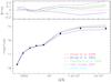 |
Fig. 2 Best solutions of the fitted isochrones to the eight-band SDSS-2MASS photometry of SDSS J102915+172927. In the upper panel we depict the solution residuals. |
The calculated best solution together with the residuals are plotted in Fig. 2 where we show the five isochrones used in this study. In Table 2 we list the parameters for each of the best solutions together with the χ2 value. In the figure the solutions overimposed on the photometric measurements are shown in the lower panel, while the residuals of the fitting are plotted in the upper panel. While for four isochrones we obtained the absolute best solutions for the distance and mass, for the Marigo et al. (2003) data our search stopped at the minimum stellar mass available, 0.70 M⊙, but clearly the fitting trend required a lower stellar mass of the order of ≃ 0.60 M⊙. Future versions of these isochrones (Bressan et al., in prep.) will allow a more precise constraint of the evolutionary status of this star.
Finally, it is not surprising to find that the best isochrone is that of Girardi et al. because it was “coloured” directly in the SDSS/2MASS systems. Our preference is the Chieffi& Limongi isochrone because it gives the lowest χ2, the best match with the spectroscopic metallicity, and with the Teff of the star (a difference of only ≃ 35° K). To summarise, the assumed distance modulus is 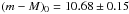 mag or 1.37 ± 0.20 kpc.
4.4. Kinematics
Kinematical data are fundamental for understanding the nature of SDSS J102915+172927. Radial velocity and proper motion measurement allowed us to compute a Galactic orbit.
4.4.1. Radial velocity
The radial velocity of the star as measured from the summed spectrum of all UVES data is −34.5 ± 1.0 km s-1, which agrees well with the −31.0 ± 10.0 km s-1measured from the X-Shooter spectrum. We found no significant variations of the radial velocity. The difference of UVES and X-Shooter is well within the given error estimates. Given the low value measured, we performed an analysis of the compatibility of the radial velocity with the different stellar populations of the Galaxy. We used the Besançon Galactic model (Robin et al. 2003) to simulate a field of 1 square degree surrounding the star. In the simulated field we selected a sample of stars with similar magnitude and colours around SDSS J102915+172927: we used a box 0.1 mag wide in both r and (r − i). The observed radial velocity lies within 1.2σ from the expected mean radial velocity of the field stellar population, thin and thick disc and halo, which has an average of +37.4 km s-1 and a σ = 58.2 km s-1. A “normal” radial velocity excludes the possibility that this star is a member of recently accreted streams or other substructures present in the halo of the Galaxy.
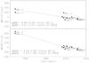 |
Fig. 3 Measurement of the proper motion in the two coordinates, RA in the bottom panel, Dec in the upper panel. The zero points for the offsets are given by the position in the SDSS-DR7 catalogue. The results of the two different fits are shown: for all positions (long dashed line) and for the positions since 1990 only (dotted line). |
4.4.2. Proper motion
Although recent surveys and old photographic catalogues have allowed us to build all-sky catalogues of proper motions for several millions of stars, subtle systematic errors are always lurking in the data, therefore we recommend caution.
In the present case the recent PPMXL Catalogue (Roeser et al. 2010) provides a proper motion measurement for this star: μαcos(δ) = −12.8 ± 3.9 mas/yr and μδ = −6.7 ± 3.9 mas/yr. The values are based on six different measurements comprising POSS I and II and 2MASS. This is not the only available measurement since also SDSS-DR7 Munn et al. (2004) provides a measurement for the proper motion: μαcos(δ) = −19 ± 2 mas/yr and μδ = −1 ± 2 mas/yr. There also seems to be a negative value for the right ascension here, but almost no motion in declination. However, the latter measurements were discovered to have systematic errors (Munn et al. 2008) that were corrected, but leave some doubt about the derived proper motions. We have to note that the faintness of the object makes it intrinsically difficult to measure in some of the surveys (like in 2MASS and UCAC3) because it is near the magnitude limit of the detectors.
To check the validity of the above values of proper motions, we independently measured the positions of the star in images of different epochs. We then combined these positions with the star’s positions in different recent astrometric catalogues based on CCD detectors. The proper motion strongly depends on the first epoch position given by the POSS-I plates taken in the 1950s. Since then there is a long gap until the 1980s. To improve the first epoch position, we recalculated the astrometry of the available photographic plates, POSS-I and POSS-II with the help of the SDSS photometry in the field. We recovered 1 × 1 deg2 images for both POSS-I/II around our target star in the blue and red from the MAST database at STScI. We then obtained a new astrometric solution for each POSS image using the SCAMP programme4. The extracted sources were compared with an SDSS-DR7 reference catalogue built by selecting only objects classified as compact galaxies with magnitude r < 21.00. A total of 2532 galaxies were used as reference out of a total of 20 532 objects present in the field. With this sample of galaxies we minimised the systematic effects present in independent astrometries. We then “swarped” each image with the SWARP programme (see footnote 4) and measured the positions with SEXTRACTOR (parameters X/Y-WIN_IMAGE and given errors). We found no significant presence of systematic trends either with position in the plate, magnitude, or type of object. We verified that the used reference galaxies defined a common zero point of the two astrometries (POSS and SDSS-DR7).
A similar procedure has been used also on the recent R- and V-band images taken at the Asiago Cima Ekar Schmidt Telescope already described above. We used the same reference list of galaxies to perform the astrometrisation of the field, again using the SCAMP/SWARP/SEXTRACTOR sequence of programmes. In this case we started for each band from the four images and “swarped” the resulting final positions with sextractor to a single image.
To the 2 POSS-I, the 2 POSS-II, and two Asiago positions we added 2MASS, UCAC3, CMC14 and, of course, SDSS-DR7 to compute the final proper motions that are shown in Fig. 3. Clearly, the entire “signal” of the proper motion is indeed given by the first epoch positions of the 2 POSS-I plates. Fitting linear regression gives a solution of μαcos(δ) = −12.33 ± 0.66 mas/yr and μδ = −6.60 ± 0.99 mas/yr, which is quite similar to the PPMXL solution. If we drop the POSS-I and use only the measurements taken after 1990.0, we find a less significant solution μαcos(δ) = −7.23 ± 1.96 mas/yr and μδ = −5.01 ± 3.00 mas/yr.
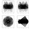 |
Fig. 4 Galactic orbit for star J102915.14+172927.9 obtained using the PPMXL proper motion. The top-left panel shows the X/Z plane; top-right shows the Y/Z plane; bottom-left shows the X/Y plane; bottom-right shows the meridional plane R/Z. |
4.4.3. Galactic orbit
Combining the positional and kinematic information, we calculated the Galactic orbit of the star by performing several tests varying the input parameters within the errors. The code used (Gratton et al. 2003) is based on the Allen & Santillan (1991) prescriptions for the Galactic potential components with updated parameters for the constants describing the potential. Although the low height on the Galactic plane (Z ~ 1.0 kpc) may suggest a thick disk orbit, this can be safely ruled out. The orbit solution indicates that the star belongs to the halo with the maximum height above the galactic plane Zmax = 4.8 ± 0.4 kpc, the orbital apocenter at Rmax = 9.6 ± 0.6 kpc, and is plunging towards the Galactic centre, with orbital pericenter Rmin = 0.9 ± 0.1 kpc. See Fig. 4. Adopting the proper motion values obtained in the previous section from the positions after 1990.0, we obtain a similar orbit with a more extreme orbital pericenter Rmin = 0.4 ± 0.1 kpc. An even more extreme value of 0.2 ± 0.1 kpc is obtained when we adopt a null value of the proper motion.
4.5. Abundances
Very few lines are measurable in the X-Shooter spectrum. The Mg i-b triplet is not visible. Of the IR Ca ii triplet lines, only the one at 854.2 nm is clearly visible, but is contaminated by a feature produced by the sky subtraction. Some Fe i lines can be guessed, not really measured. The only clearly detectable line is the Ca ii-K line at 393.3 nm. Its EW of 49.2 pm is consistent with an abundance of [Ca/H ] = −3.9. But the measured radial velocity is –30 km s-1, comparable to the X-Shooter UBV arm resolution of 7900, which suggests that the line is contaminated by the component from the interstellar medium (ISM). From the X-Shooter spectrum, we can deduce that this spectrum belongs to an extremely metal-poor star and put an upper limit on the metallicity of about –4.0 with respect to the solar metallicity.
The UVES spectrum resolves the stellar and IS components of the Ca ii-K and Ca ii-H line (see Fig. 5). The EW of the stellar Ca ii-K line is of 27.7 pm, corresponding to an abundance of [Ca/H ] = −4.47. We did not take this line as an abundance indicator, because it is difficult to separate the stellar and IS components, and because with an EW of 27.7 pm this line is saturated and not very sensitive to abundance.
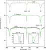 |
Fig. 5 Range of the Ca ii H and K lines. From top to bottom, SDSS, X-Shooter, and UVES spectrum (solid black), overimposed the synthetic profile with metallicity –4.5, α-enhanced by 0.4 dex (solid green). |
In the UVES spectrum we can see lines of iron peak elements (Fe i, Ni i) and α-elements (Mg i, Si i, Ca i, Ca ii, Ti ii). For the light elements Li and C-N we were unable to find an evident signature in the spectra, therefore we can provide only an upper-limit.
For the abundance determination we relied on line profile fitting because some lines happen to be blended (sometimes several lines of the same element) and some lines lie on the wings of hydrogen lines. We computed a grid of synthetic spectra with the effective temperature and gravity of the star, varying in [Fe/H] by 0.2 dex. We fitted the Fe i features to derive the 1D-LTE [Fe/H]. To derive the abundances of the other elements, we computed grids of synthetic spectra with fixed [Fe/H], by varying the abundance [X/Fe] of the element X by 0.2 dex and then by fitting the line profiles. The abundances derived for all elements are reported in Table 3. The differences with respect to Table 1 of Caffau et al. (2011c) are that we use a different 3D model atmosphere and the applications of NLTE.
4.6. The Li abundance
A 3D-NLTE (Sbordone et al. 2010) Li abundance of 2.2 (Spite plateau) would imply an EW for the Li doublet at 670.7 nm of about 4.7 pm in this star. Such a feature should be visible in the observed spectra, but no sign of the line is detectable in the expected wavelength range. In the X-Shooter spectrum, taking into account its signal-to-noise ratio (S/N) and the resolution, we expect according Cayrel’s formula (Cayrel 1988) that the limit for a feature to be visible is about 1.5 pm (3σ), which would correspond to a A(Li) = 1.7, close to the Li abundance derived for the cooler component of the binary system CS 22876-32 (González Hernández et al. 2008). From the S/N of the UVES spectrum (160) an upper limit on the EW of 0.1 pm implies A(Li) < 1.1 at 5σ or A(Li) < 0.9 at 3σ.
SDSS J102915+172927.
This implies that the star is far below the Spite plateau. This may be linked to the fact that at extremely low metallicities the Spite plateau displays a “meltdown” (Sbordone et al. 2010), i.e. an increased scatter and a lower mean Li abundance. This meltdown is clearly visible in the two components of the extremely metal-poor binary system CS 22876-32 ( [Fe/H ] = −3.6, the primary with an effective temperature of 6500 K, the secondary of 5900 K), which show a different Li content (González Hernández et al. 2008). The primary lies on the Spite plateau, while the secondary lies below at A(Li) = 1.8. The reasons for this meltdown are not understood. It has been suggested that a Li depletion mechanism, whose efficiency is metallicity-dependent, might be able to explain the observations. If this were the case, the Li abundance in SDSS J102915+172927 would result from an efficient Li depletion caused by a combination of extremely low metallicity and relatively low temperature. If the star were a horizontal branch star (Hansen et al. 2011), it would be normal for it to be Li depleted. However, we already argued that low gravities, compatible with an HB status, are ruled out. A sub-giant status should not imply a high Li depletion. The absence of Li could be explained if SDSS J102915+172927 were a “blue straggler to be” (Ryan et al. 2002). In this case we would expect a measurable line broadening owing to rotation. In our UVES spectra we cannot derive any line broadening above what is caused by the instrumental resolution, which is set by the seeing. Therefore all available evidence suggests that SDSS J102915+172927 is in an evolutionary status from the main sequence to the sub-giant branch.
4.7. CNO upper limits
No strong carbon enhancement is evident in the UVES spectrum (see Fig. 6). We fitted the range of the G-band at 430 nm, and found [C/H]1D = −3.81. The S/N in the range is of about 70. The same fit of a synthetic spectrum with S/N of 50 gives [C/H ] = −4.25, C-enhancement of 0.25 dex with respect to the input value. We consider [C/H] < −3.81 as an upper limit. If we applied 3D corrections, the abundance decreased and the upper limit became more strict. This is because the temperature structure of a 3D model is cooler than the reference 1D model in the external layers. In these cooler layers, the formation of molecules is favoured, which means that with the same abundance the observed molecular bands are deeper which in turn implies a lower abundance, see González Hernández et al. (2010) and Behara et al. (2010) for details.
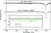 |
Fig. 6 G-band range of the the star SDSS J102915+172927: the observed spectrum (solid black) is compared to the known C-enhanced star HE 1327-2326. A zoom on the G-band is shown (solid black) compared to the best fit of the range (solid red) and with a synthetic profile enhanced in C by 2 dex (solid green). |
For the nitrogen we investigated the NH band at 336 nm. We found no evidence of enhancement (see Fig. 7) here either; when we fited the range we obtained an upper limit of an N-enhancement of 0.24 dex. As for the G-band, we consider this value as an upper limit for nitrogen. The 3D corrections would imply a lower upper limit for this molecule as well.
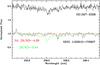 |
Fig. 7 NH-band range of the the star SDSS J102915+172927: the observed spectrum (solid black) is compared to the best fit of the range (solid green) and with a synthetic profile enhanced in N by 2 dex (solid green). For comparison the known N-enhanced star HE 1327-2326 is shown. |
SDSS J102915+172927, with a metallicity of Z = 5 × 10⁻⁵ Z⊙, is the presently known object whose composition closest resembles the primordial one. We computed the metallicity with the 1D abundances derived from the UVES spectrum, the 1D C and N upper limits that we derived by fitting the molecular bands of CH and NH, respectively, and assuming an enhancement in oxygen of [O/Fe ] = + 0.6.
4.8. Non-LTE effects on the element abundance determinations
Our present investigation is based on the non-local thermodynamic equilibrium (non-LTE) line formation for six chemical species. We used the non-LTE methods treated in our earlier studies and documented in a number of papers, in which atomic data and the problems of line formation were considered in detail, i.e., in Zhao et al. (1998, Mg i, Shi et al. (2008, Si i, Mashonkina et al. (2007, Ca i-Ca ii, Mashonkina et al. (2011, Fe i, and Belyakova & Mashonkina (1997, Sr ii. To solve the coupled radiative transfer and statistical equilibrium (SE) equations, we used a revised version of the DETAIL programme (Butler & Giddings 1985) based on the accelerated lambda iteration, which follows the efficient method described by Rybicki & Hummer (1991, 1992). The non-LTE calculations were performed for the ATLAS 9 atmospheric structure.
It is worth noting that we used the most accurate atomic data for each chemical species. Photoionisation cross-sections are from the opacity project (OP) calculations (Seaton et al. 1994). Their accuracy is estimated at the level of 10%. This small uncertainty translates into an abundance error of no more than 0.01 dex. When no OP data are available for Sr ii, we ignore photoionisation since it affects its SE only weakly because Sr iii is an extremely small fraction of the total strontium atoms. The atomic data for Ca ii were updated by applying effective collision strengths from the R-matrix calculations of Meléndez et al. (2007). We accounted for inelastic collisions both with electrons and neutral H particles in SE calculations. Hydrogen collisions were computed using the formula of Steenbock & Holweger (1984) with a scaling factor SH = 0.1 and 1. For Ca i-Ca ii and Fe i-Fe ii our favourite is SH = 0.1 as estimated empirically from the different influence of hydrogen atom collisions on the different lines of a given atom in solar and stellar spectra (Mashonkina et al. 2007, 2011). For Sr ii, we applied SH = 0 (no hydrogenic collisions), as recommended by Mashonkina & Gehren (2001).
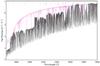 |
Fig. 8 Emerging fluxes calculated using the 5811/4/−4.5 (solid black) and 5780/4.44/0 (dotted violet) model. Bold marks indicate the thresholds of the Fe i levels with excitation energy of 0.9 to 3.7 eV. |
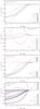 |
Fig. 9 Departure coefficients b, for the selected levels of the investigated atoms as a function of log τ5000 in the model atmosphere 5811/4.0/−4.5. Bottom panel: we show every fifth of the first 60 levels for Fe i. They are quoted in the bottom-right part of the panel. All remaining higher levels of Fe i are plotted by dotted curves. We show the same for Fe ii. They are quoted in the top-right part of the panel. SH = 0.1 throughout. |
The main non-LTE mechanism for the minority species in the model 5811/4.0/−4.5, Mg i, Si i, Ca i, and Fe i, is the overionisation caused by superthermal radiation of non-local origin below the thresholds of the levels with Eexc = 2.2–4.5 eV (λthr = 2240−3450 Å). In the extremely metal-poor atmosphere, deviations of the mean intensity of ionizing ultraviolet radiation from the Planck function are more pronounced compared with those of the solar metallicity model (Fig. 8), resulting in much stronger departures from LTE. Figure 9 shows that all levels of Mg i, Ca i, and Fe i and the three lowest levels of Si i are strongly underpopulated in the line formation layers of the 5811/4.0/ − 4.5 model. Here we use the departure coefficients  , where
  and
and  are the statistical equilibrium and thermal (Saha-Boltzmann) number densities, respectively. Non-LTE leads to a weakening of the Mg i, Si i, Ca i, and Fe i lines and positive non-LTE abundance corrections ΔNLTE = log εNLTE − log εLTE. We comment on the obtained results for individual species.
The observed Mg i lines arise in the transitions – (382.9–383.8 nm) and – (517.2, 518.3 nm). For each line, the upper level is depleted to a lesser extent with regard to its LTE population than the lower level. Therefore, the line is weaker compared with its LTE strength not only because of the general overionisation (bl < 1), but also because the line source function (Slu ≃ bu/bl Bν) rises above the Planck function (Bν) in the line formation layers. Here, bu and bl are the departure coefficients of the upper and lower levels, respectively. All investigated lines have similar non-LTE abundance correction at the level of +0.2 dex from the calculations with SH = 0.1 (Table 4). As expected, the departures from LTE are reduced for increased H i collision rates (SH = 1).
The effect of bu/bl > 1 resulting in Slu > Bν is more prominent for the only available line of silicon, Si i 390.5 nm. Its lower level follows the ground state of Si i inside log τ5000 < −1.5 due to collisional coupling, and it is strongly underpopulated in the line formation layers. Its coupling to the high-excitation levels for the upper level turns out to be stronger than a coupling to the lower excitation levels, and tends to follow the continuum, Si ii. This explains why Si i 390.5 nm has a larger non-LTE correction of ΔNLTE = 0.34 dex (SH = 0.1) compared to the corresponding values for the Mg i lines and why ΔNLTE is only slightly reduced when moving to SH = 1 (Table 4).
For the resonance line of Ca i at 422.6 nm, the non-LTE mechanisms are very similar to those of the Mg i lines. Calcium is the only element observed in SDSS J102915+172927 in two ionisation stages. Ca ii dominates the element number density over atmospheric depths. Therefore, no process seems to affect the Ca ii ground-state population, and 4s keeps its thermodynamic equilibrium value. The levels 3d and 4p follow the ground state in deep layers, and their coupling is lost at the depths outside log τ5000 < −1 where photon losses in the weakest line 849.8 nm of the multiplet 3d − 4p start to become important. In these atmospheric layers, bu/bl < 1 is valid for each investigated line of Ca ii resulting in dropping the line source function above the Planck function and enhanced line absorption. For the resonance line Ca ii 393.3 nm, departures from LTE occur only in the very core and ΔNLTE amounts to − 0.07 dex. Non-LTE correction is larger in absolute value for the IR lines of multiplet 3d − 4p, 849.8, 854.2, and 866.2 because of the overpopulation of the lower level.
Weakening of the Fe i lines is mainly due to overionisation. In SDSS J102915+172927, we measured only the low-excitation Fe i lines, with Eexc = 0-1.5 eV. The source function is quite similar to the Planck function for each investigated line, because all levels with Eexc = 0-4.5 eV behave similarly (Fig. 9). With the very similar behaviour of the departure coefficients for the lower levels, we calculated very similar non-LTE corrections, as can be seen in Fig. 10. ΔNLTE varies between 0.29 and 0.36 dex in the calculations SH = 0.1. Similarly to the Mg i lines, the departures from LTE are reduced significantly for SH = 1, see Table 4.
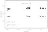 |
Fig. 10 Non-LTE abundance corrections for the Fe i lines in the 5811/4.0/–4.5 model depending on Eexc from the calculations with SH = 0.1 (filled circles) and SH = 1 (triangles). |
Although only an upper limit was estimated for the Sr abundance, we performed the non-LTE calculations for Sr ii with [Sr/Fe] = −5.1. Non-LTE leads to a weakened Sr ii 407.7 nm line, and ΔNLTE amounts to 0.16 dex if pure electronic collisions are taken into account in the SE calculations and decreases down to 0.12 dex for SH = 1. For Ti ii, we estimated a non-LTE correction of –0.01 dex, assuming that the departures from LTE for the investigated Ti ii lines are similar to those of the Fe ii lines of similar excitation energy and equivalent width.
Non-LTE abundance corrections (dex) for the lines in SDSS J102915+172927 depending on surface gravity.
5. The ISM towards the star SDSS J102915+172927
The spectrum of SDSS J102915+172927 shows interstellar absorptions of the Na i D-line doublet at 589.0 nm (see Fig. 11) and the Ca ii-K line at 393.3 nm and Ca ii-H line at 396.8 nm (see detail inside Fig. 5).
The interstellar feature is satisfactory modelled with one single component model providing a column density of log (Na i) = 12.11 ± 0.01 cm-2 and log (Ca ii) = 12.02 ± 0.04 cm-2. The broadening of the lines is 7.3 ± 1.1 km s-1 in the Ca ii lines and 5.2 ± 0.1 km s-1 in Na i, suggesting that the turbulence is the dominant broadening factor and that the two ions do not sample precisely the same material with the Ca ii lines tracing ionised gas not detected in Na i.
The Na i column density is consistent with that observed towards η Leo, which at an angular distance of a few degrees shows log N(Na i) = 12.08 cm-2.
High spectral resolution absorption observations of the local neutral and partially ionised interstellar gas using both the Na i D-line doublet and the Ca ii-K line allowed us to construct a picture of the distribution of neutral gas in the local interstellar medium. The Sun is placed within a low density interstellar cavity connected by interstellar tunnels to other surrounding cavities.
Welsh et al. (2010) reported on the results of an extended survey of Na i and Ca ii absorption lines recorded at high spectral resolution towards thousands of early-type stars mostly located within 800 pc of the Sun. In particular, maps of the distribution of Na i absorption revealed that the local cavity has a 50 pc diameter and a 200 pc long extension in the direction of the star β CMa and that there is an extension of rarefied gas into the lower galactic halo that forms an open-ended chimney feature.
The line of sight towards SDSS J102915+172927 has the galactic coordinates l = 222.7 and b = 56 i.e. lying in the third quadrant and at fairly high latitudes, intercepting low-density material.
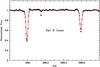 |
Fig. 11 IS lines of Na i in the spectrum of SDSS J102915+172927. A telluric absorption line is denoted by a crossed circle. The solid line is a synthesis of the IS one-component model. |
The observed column density ratio in the line of sight towards SDSS J102915+172927 is N(Na i)/N(Ca ii) = 1.1. This ratio is a diagnostic of the physical conditions in the diffuse interstellar gas. In cold (T ~ 30 K) and dense gas clouds most of the gas-phase Ca is depleted onto grains, and the Na i/Ca ii ratio is ≪ 1. In warmer (T ~ 1000 K) and lower density ISM much of the Ca remains in the gas phase, and ratios of < 1.0 are commonly found. For instance, for sight-line distances inside the local cloud the Na i/Ca ii column density ratio for the warm (T ~ 7000 K) local interstellar gas clouds is ~0.2. The Na i/Ca ii ratio is thought to be also connected to the gas cloud velocity, such that at velocities ≥30 km s-1 interstellar dust grains may be destroyed by shocks and Ca is liberated into the gas phase (Routly & Spitzer 1952). Accordingly, a low value of the Na i/Ca ii ratio could be due either to the presence of warm and partially ionised gas and/or the presence of interstellar shocks. Since we do not observe high velocities, the observed low Na i/Ca ii ratio is most probably caused by significant amounts of partially ionised Ca ii gas.
The Na i/Ca ii ratio value generally falls in the range 0.5 to 20 but with a smaller range of ratio values, between 0.1 to 5, in quadrant 3 where our line of sight lies, and it matches the value measured towards SDSS J102915+172927.
By using Na i as a tracer of neutral hydrogen, we can infer a total column density of log N(H) = 20.38 cm-2 (Ferlet et al. 1985). This column density is similar to that of log N(H) = 20.43 cm-2 directly measured in ρ Leo from the Lyα absorption line by means of IUE spectra (Shull & Van Steenberg 1985). Because this is located at a distance of 950 pc, the gas column densities place a robust lower limit to the distance of SDSS J102915+172927.
With the given hydrogen column density the extinction is Av = 0.13, and assuming an extinction-to-reddening ratio of Av/E(B − V) = 3.1, we obtain E(B − V) = 0.04, which is quite consistent with the extinction value as deduced from extinction maps.
6. Discussion
The sample of EMP candidates selected from the SDSS archive (see details in Caffau et al. 2011b), and observed with the high-efficiency spectrographs X-Shooter (Caffau et al. 2011b), or UVES (Bonifacio et al. 2012) is confirmed by this discovery to contain stars at the lowest levels of metallicity observed in the Galaxy. The few stars selected from SDSS and observed at high resolution cannot allow us to assess the real efficiency of the method, but this could be achieved with more observations.
This discovery gives our understanding of the formation of the first generations of stars a new perspective. The level of chemical enrichment of a star is characterised by the global metallicity Z. The most metal-poor stars formerly known had a metallicity of about Z = 10-3.5 Z⊙, while SDSS J102915+172927 has a metallicity Z ≤ 10-4.0 Z⊙. A few stars with extremely low iron abundances (of the order of [Fe/H ] = −5.0 or lower, Christlieb et al. 2002; Frebel et al. 2005; Norris et al. 2007) were discovered in the past decade. However, their chemical composition is highly peculiar, with C, N, and O being more abundant than expected with respect to iron by several orders of magnitude, corresponding to a moderately low Z, of the order of 10-2 Z⊙. This state of affairs supported the notion that the first generations of stars were formed exclusively by extremely massive stars (now long extinct) and that there exists a critical metallicity below which low-mass stars cannot form (Bromm & Loeb 2003; Schneider et al. 2003). The existence of SDSS J102915+172927 demonstrates that either such a critical metallicity does not exist, in line with the scenario of Greif et al. (2011), or that it is lower than 10-4 Z⊙, in line with the scenario of Schneider et al. (2003). The peculiar chemical composition of HE 0107-5240 and HE 1327-2326 is consistent with the picture by Frebel et al. (2007), using the Bromm & Loeb (2003) theory, in which the critical parameter is not metallicity, but a suitable combination of C and O abundances. The fact that SDSS J102915+172927 is not carbon-enhanced places this star in what this theory calls the “forbidden zone”. We have no upper limit on the oxygen abundance, but because C, N, and Mg are not enhanced (as they are in HE 0107-5240 and HE 1327-2326), there is no reason to suspect any significant O enhancement. If we assume, conservatively, [O/H] ≤ −4.1 and [C/H] ≤ − 3.8, the transition discriminant5 is D ≤ −3.7, while low-mass star formation should only be possible for D ≥ −3.5. Our discovery will a give new impulse to the formation theories of low-metallicity stars. The notion of critical metallicity or metallicity discriminant may have to be revisited.
The properties of SDSS J102915+172927 are compatible with the protogalaxy scenario discussed in Omukai et al. (2008). In this case, metal-poor gas under extreme UV irradiation, with a normal dust-to-gas ratio and with a metallicity of Z > 5 × 10⁻⁶ of Z⊙, fragments into a dense cluster of sub-solar mass stars (see their Fig. 5). This particular way of forming low-mass metal-poor stars does not require any C/N/O enhancement, because of the peculiar thermal evolution of the gas. Also Schneider et al. (2012) expect formation of stars as metal-poor as SDSS J102915+172927, and the cooling of the gas cloud is due to dust. In both cases a minimum metallicity is expected for low-mass star formation. On the other hand, the fragmentation found by the simulations of Clark et al. (2011) relies on H2 cooling and requires no metal enrichment. If the IMF of the primordial stars is indeed flat, as found by Greif et al. (2011), then we may expect to find low-mass stars even more metal-poor than SDSS J102915+172927 and, possibly, of primordial metallicity. One concern on the observability of these primordial stars is the possibility that their atmospheres may have been polluted by metals during encounters with molecular clouds during their long lifetimes. While early estimations of this process predicted significant pollution to take place (Yoshii et al. 1995), subsequent observations failed to detect the predicted “accretion plateau” of light elements (Molaro et al. 1997; Boesgaard et al. 1999; Smiljanic et al. 2009; Duncan et al. 1997; Garcia Lopez et al. 1998). More recent estimations of the accretion process efficiency (Frebel et al. 2009) seem to exclude any significant pollution, especially if the primordial stars have a weak solar-like wind (Johnson & Khochfar 2011). These considerations should encourage an extensive search for more stars that are as metal-poor as SDSS J102915+172927 or even more metal-poor.
Increasing the number of stars at these very low metallicities will also help understanding the behaviour of lithium at extremely low metallicities. If below a given metallicity low-mass stars can only be formed by fragmentation of larger collapsing clouds (Clark et al. 2011; Greif et al. 2011), a distinct possibility is that this process results in turbulence and/or rotation fast enough to destroy the primordial lithium originally present in the gas effectively during the pre-main sequence phase. In this scenario we expect all stars below a given metallicity to show no lithium. As star formation begins to proceed in a more conventional way, through metal-line cooling, the stars do not destroy the lithium, and the Spite plateau appears. The Spite plateau meltdown (Sbordone et al. 2010) could simply mark a transition region between the two regimes of star-formation.
The original version is available on-line at http://kurucz.harvard.edu/.
E. Bertin, see for details http://www.astromatic.net/
Dtrans = log (10 [C/H ] + 0.3 × 10 [O/H ] ).
Acknowledgments
The authors would like to thank A. Chieffi and M. Limongi, who kindly provided a set of unpublished isochrones. The authors thank M. Barbieri for providing the Galactic model for the orbit calculations and for many useful discussions. We are grateful to R. Scholz for useful discussions on the proper motion measurements. We also thank P. Ochner for the observations at the Asiago telescope. E. Caffau and P. Bonifacio wish to thank ESO for the hospitality at ESO-Santiago provided during the preparation of the paper. P. Bonifacio, P. François, M. Spite, F. Spite, R. Cayrel, B. Plez and V. Hill acknowledge support from the Programme National de Physique Stellaire (PNPS) and the Programme National de Cosmologie et Galaxies (PNCG) of the Institut National de Sciences de l’Universe of CNRS. This paper is also based on observations collected at the Asiago Observatory (Italy). L. Mashonkina is supported by the Presidium RAS Programme “Origin, structure, and evolution of cosmic objects” (No. P-19) and the Swiss National Science Foundation (SCOPES project No. IZ73Z0-128180/1). H.G.L. acknowledges financial support by the Sonderforschungsbereich SFB 881 “The Milky Way System” (subproject A4) of the German Research Foundation (DFG). The authors would like to thank the anonymous referee for the useful suggestions.
References
- Allen, C., & Santillan, A. 1991, RMA&A, 22, 255 [Google Scholar]
- Alonso, A., Arribas, S., & Martinez-Roger, C. 1996, A&A, 313, 873 [NASA ADS] [Google Scholar]
- Barklem, P. S., Piskunov, N., & O’Mara, B. J. 2000a, A&A, 355, L5 [NASA ADS] [Google Scholar]
- Barklem, P. S., Piskunov, N., & O’Mara, B. J. 2000b, A&A, 363, 1091 [NASA ADS] [Google Scholar]
- Behara, N. T., Bonifacio, P., Ludwig, H.-G., et al. 2010, A&A, 513, A72 [NASA ADS] [CrossRef] [EDP Sciences] [Google Scholar]
- Beers, T. C. 1999, Ap&SS, 265, 547 [NASA ADS] [CrossRef] [Google Scholar]
- Beers, T. C., Preston, G. W., & Shectman, S. A. 1985, AJ, 90, 2089 [NASA ADS] [CrossRef] [Google Scholar]
- Beers, T. C., Preston, G. W., & Shectman, S. A. 1992, AJ, 103, 1987 [NASA ADS] [CrossRef] [Google Scholar]
- Belyakova, E. V., & Mashonkina, L. I. 1997, Astron. Rep., 41, 530 [NASA ADS] [Google Scholar]
- Boesgaard, A. M., Deliyannis, C. P., King, J. R., et al. 1999, AJ, 117, 1549 [NASA ADS] [CrossRef] [Google Scholar]
- Bonifacio, P., & Caffau, E. 2003, A&A, 399, 1183 [NASA ADS] [CrossRef] [EDP Sciences] [Google Scholar]
- Bonifacio, P., Spite, M., Cayrel, R., et al. 2009, A&A, 501, 519 [NASA ADS] [CrossRef] [EDP Sciences] [Google Scholar]
- Bonifacio, P., Caffau, E., François, P., et al. 2011a, Astron. Nachr., 332, 251 [NASA ADS] [CrossRef] [Google Scholar]
- Bonifacio, P., Sbordone, L., Caffau, E., et al. 2012, A&A, in press, DOI: 1051/0004-6361/201219004 [Google Scholar]
- Bromm, V., & Loeb, A. 2003, Nature, 425, 812 [NASA ADS] [CrossRef] [EDP Sciences] [PubMed] [Google Scholar]
- Butler, K., & Giddings, J. 1985, Newsletter on the analysis of astronomical spectra, No. 9, University of London [Google Scholar]
- Caffau, E., Bonifacio, P., Faraggiana, R., et al. 2005, A&A, 441, 533 [NASA ADS] [CrossRef] [EDP Sciences] [Google Scholar]
- Caffau, E., Ludwig, H.-G., Steffen, M., Freytag, B., & Bonifacio, P. 2011a, Sol. Phys., 268, 255 [NASA ADS] [CrossRef] [Google Scholar]
- Caffau, E., Bonifacio, P., François, P., et al. 2011b, A&A, 534, A4 [NASA ADS] [CrossRef] [EDP Sciences] [Google Scholar]
- Caffau, E., Bonifacio, P., François, P., et al. 2011c, Nature, 477, 67 [NASA ADS] [CrossRef] [PubMed] [Google Scholar]
- Castelli, F., & Kurucz, R. L. 2004, Proc. IAU Symp. 210, poster A20 [arXiv:astro-ph/0405087] [Google Scholar]
- Cayrel, R. 1988, The Impact of Very High S/N Spectroscopy on Stellar Physics, IAU Symp., 132, 345 [NASA ADS] [CrossRef] [Google Scholar]
- Cayrel, R., Depagne, E., Spite, M., et al. 2004, A&A, 416, 1117 [NASA ADS] [CrossRef] [EDP Sciences] [Google Scholar]
- Christlieb, N., Bessell, M. S., Beers, T. C., et al. 2002, Nature, 419, 904 [NASA ADS] [CrossRef] [PubMed] [Google Scholar]
- Christlieb, N., Schörck, T., Frebel, A., et al. 2008, A&A, 484, 721 [NASA ADS] [CrossRef] [EDP Sciences] [Google Scholar]
- Clark, P. C., Glover, S. C. O., Smith, R. J., et al. 2011, Science, 331, 1040 [NASA ADS] [CrossRef] [PubMed] [Google Scholar]
- Dekker, H., D’Odorico, S., Kaufer, A., Delabre, B., & Kotzlowski, H. 2000, Proc. SPIE, 4008, 534 [Google Scholar]
- D’Odorico, S., Dekker, H., Mazzoleni, R., et al. 2006, Proc. SPIE, 6269E, 98 [NASA ADS] [Google Scholar]
- Duncan, D. K., Primas, F., Rebull, L. M., et al. 1997, ApJ, 488, 338 [NASA ADS] [CrossRef] [Google Scholar]
- Edvardsson, B., Andersen, J., Gustafsson, B., et al. 1993, A&A, 275, 101 [NASA ADS] [Google Scholar]
- Ferlet, R., Vidal-Madjar, A., & Gry, C. 1985, ApJ, 298, 838 [NASA ADS] [CrossRef] [Google Scholar]
- François, P., Depagne, E., Hill, V., et al. 2007, A&A, 476, 935 [NASA ADS] [CrossRef] [EDP Sciences] [Google Scholar]
- Frebel, A., Aoki, W., Christlieb, N., et al. 2005, Nature, 434, 871 [NASA ADS] [CrossRef] [PubMed] [Google Scholar]
- Frebel, A., Johnson, J. L., & Bromm, V. 2007, MNRAS, 380, L40 [NASA ADS] [CrossRef] [Google Scholar]
- Frebel, A., Johnson, J. L., & Bromm, V. 2009, MNRAS, 392, L50 [NASA ADS] [Google Scholar]
- Freytag, B., Steffen, M., Ludwig, H.-G., et al. 2012, J. Comp. Phys., 231, 919 [Google Scholar]
- Fukugita, M., Ichikawa, T., Gunn, J. E., et al. 1996, AJ, 111, 1748 [NASA ADS] [CrossRef] [Google Scholar]
- Garcia Lopez, R. J., Lambert, D. L., Edvardsson, B., et al. 1998, ApJ, 500, 241 [NASA ADS] [CrossRef] [Google Scholar]
- Girardi, L., Bertelli, G., Bressan, A., et al. 2002, A&A, 391, 195 [NASA ADS] [CrossRef] [EDP Sciences] [Google Scholar]
- Girardi, L., Grebel, E. K., Odenkirchen, M., & Chiosi, C. 2004, A&A, 422, 205 [NASA ADS] [CrossRef] [EDP Sciences] [Google Scholar]
- Girardi, L., Groenewegen, M. A. T., Hatziminaoglou, E., & da Costa, L. 2005, A&A, 436, 895 [NASA ADS] [CrossRef] [EDP Sciences] [Google Scholar]
- Goldoni, P., Royer, F., François, P., et al. 2006, Proc. SPIE, 6269, 80 [NASA ADS] [Google Scholar]
- González Hernández, J. I., & Bonifacio, P. 2009, A&A, 497, 497 [NASA ADS] [CrossRef] [EDP Sciences] [Google Scholar]
- González Hernández, J. I., Bonifacio, P., Ludwig, H.-G., et al. 2008, A&A, 480, 233 [NASA ADS] [CrossRef] [EDP Sciences] [MathSciNet] [Google Scholar]
- González Hernández, J. I., Bonifacio, P., Ludwig, H.-G., et al. 2010, A&A, 519, A46 [NASA ADS] [CrossRef] [EDP Sciences] [Google Scholar]
- Gratton, R. G., Carretta, E., Claudi, R., Lucatello, S., & Barbieri, M. 2003, A&A, 404, 187 [NASA ADS] [CrossRef] [EDP Sciences] [Google Scholar]
- Greif, T. H., Springel, V., White, S. D. M., et al. 2011, ApJ, 737, 75 [NASA ADS] [CrossRef] [Google Scholar]
- Gustafsson, B., Edvardsson, B., Eriksson, K., et al. 2003, Proc. IAU Symp. 210, poster A4 [Google Scholar]
- Gustafsson, B., Edvardsson, B., Eriksson, K., et al. 2008, A&A, 486, 951 [NASA ADS] [CrossRef] [EDP Sciences] [Google Scholar]
- Hansen, C. J., Nordström, B., Bonifacio, P., et al. 2011, A&A, 527, A65 [NASA ADS] [CrossRef] [EDP Sciences] [Google Scholar]
- Johnson, J. L., & Khochfar, S. 2011, MNRAS, 413, 1184 [Google Scholar]
- Kelson, D. D., PASP, 115, 688 [Google Scholar]
- Kurucz, R. 1993, ATLAS9 Stellar Atmosphere Programs and 2 km s-1 grid CD-ROM No. 13, Cambridge, Mass.: Smithsonian Astrophysical Observatory [Google Scholar]
- Kurucz, R. L. 2005, Mem. Soc. Astron. Ital. Suppl., 8, 14 [Google Scholar]
- Lodders, K., Plame, H., & Gail, H.-P. 2009, Science and Technology, 4B, 44 [Google Scholar]
- Ludwig, H.-G., Bonifacio, P., Caffau, E., et al. 2008, Phys. Scr. T, 133, 014037 [Google Scholar]
- Ludwig, H.-G., Caffau, E., Steffen, M., et al. 2009, Mem. Soc. Astron. Ital., 80, 711 [Google Scholar]
- Marigo, P., Chiosi, C., & Kudritzki, R.-P. 2003, A&A, 399, 617 [NASA ADS] [CrossRef] [EDP Sciences] [Google Scholar]
- Mashonkina, L., & Gehren, T. 2001, A&A, 376, 232 [NASA ADS] [CrossRef] [EDP Sciences] [Google Scholar]
- Mashonkina, L., Korn, A. J., & Przybilla, N. 2007, A&A, 461, 261 [NASA ADS] [CrossRef] [EDP Sciences] [Google Scholar]
- Mashonkina, L., Gehren, T., Shi, J.-R., Korn, A. J., & Grupp, F. 2011, A&A, 528, A87 [NASA ADS] [CrossRef] [EDP Sciences] [Google Scholar]
- Meléndez, M., Bautista, M. A., & Badnell, N. R. 2007, A&A, 469, 1203 [NASA ADS] [CrossRef] [EDP Sciences] [Google Scholar]
- Molaro, P., Bonifacio, P., Castelli, F., & Pasquini, L. 1997, A&A, 319, 593 [NASA ADS] [Google Scholar]
- Munn, J. A., Monet, D. G., Levine, S. E., et al. 2004, AJ, 127, 3034 [NASA ADS] [CrossRef] [Google Scholar]
- Munn, J. A., Monet, D. G., Levine, S. E., et al. 2008, AJ, 136, 895 [NASA ADS] [CrossRef] [Google Scholar]
- Nakamura, F., & Umemura, M. 2001, ApJ, 548, 19 [NASA ADS] [CrossRef] [Google Scholar]
- Norris, J. E., Christlieb, N., Korn, A. J., et al. 2007, ApJ, 670, 774 [NASA ADS] [CrossRef] [Google Scholar]
- Omukai, K., Schneider, R., & Haiman, Z. 2008, ApJ, 686, 801 [NASA ADS] [CrossRef] [Google Scholar]
- Ostriker, J. P., & Gnedin, N. Y. 1996, ApJ, 472, L63 [NASA ADS] [CrossRef] [Google Scholar]
- Robin, A. C., Reylé, C., Derrière, S., & Picaud, S. 2003, A&A, 409, 523 [NASA ADS] [CrossRef] [EDP Sciences] [Google Scholar]
- Roeser, S., Demleitner, M., & Schilbach, E. 2010, AJ, 139, 2440 [NASA ADS] [CrossRef] [Google Scholar]
- Routly, P., & Spitzer, L. 1952, ApJ, 115, 227 [NASA ADS] [CrossRef] [Google Scholar]
- Ryan, S. G., Gregory, S. G., Kolb, U., Beers, T. C., & Kajino, T. 2002, ApJ, 571, 501 [NASA ADS] [CrossRef] [Google Scholar]
- Rybicki, G. B., & Hummer, D. G. 1991, A&A, 245, 171 [NASA ADS] [Google Scholar]
- Rybicki, G. B., & Hummer, D. G. 1992, A&A, 262, 209 [NASA ADS] [Google Scholar]
- Sbordone, L. 2005, Mem. Soc. Astron. Ital. Suppl., 8, 61 [Google Scholar]
- Sbordone, L., Bonifacio, P., Castelli, F., & Kurucz, R. L. 2004, Mem. Soc. Astron. Ital. Suppl., 5, 93 [Google Scholar]
- Sbordone, L., Bonifacio, P., Caffau, E., et al. 2010, A&A, 522, A26 [NASA ADS] [CrossRef] [EDP Sciences] [Google Scholar]
- Schneider, R., Ferrara, A., Salvaterra, R., Omukai, K., & Bromm, V. 2003, Nature, 422, 869 [NASA ADS] [CrossRef] [PubMed] [Google Scholar]
- Schneider, R., Omukai, K., Bianchi, S., & Valiante, R. 2012, MNRAS, 419, 1566 [NASA ADS] [CrossRef] [Google Scholar]
- Seaton, M. J., Yan, Y., Mihalas, D., & Pradhan, A. K. 1994, MNRAS, 266, 805 [NASA ADS] [CrossRef] [Google Scholar]
- Shi, J. R., Gehren, T., Butler, K., Mashonkina, L. I., & Zhao, G. 2008, A&A, 486, 303 [NASA ADS] [CrossRef] [EDP Sciences] [Google Scholar]
- Shull, J. M., & Van Steenberg 1985, ApJ, 294, 599 [NASA ADS] [CrossRef] [Google Scholar]
- Smiljanic, R., Pasquini, L., Bonifacio, P., et al. 2009, A&A, 499, 103 [NASA ADS] [CrossRef] [EDP Sciences] [Google Scholar]
- Steenbock, W., & Holweger, H. 1984, A&A, 130, 319 [NASA ADS] [Google Scholar]
- Stehlé, C., & Hutcheon, R. 1999, A&AS, 140, 93 [NASA ADS] [CrossRef] [EDP Sciences] [Google Scholar]
- Stetson, P. B. 1987, PASP, 99, 191 [NASA ADS] [CrossRef] [Google Scholar]
- Straniero, O., Chieffi, A., & Limongi, M. 1997, ApJ, 490, 425 [NASA ADS] [CrossRef] [Google Scholar]
- Theodosiou, C. E. 1989, Phys. Rev. A, 39, 4880 [NASA ADS] [CrossRef] [Google Scholar]
- Van Dokkum, P. G. 2001, PASP, 113, 1420 [NASA ADS] [CrossRef] [Google Scholar]
- Yoshii, Y., Mathews, G. J., & Kajino, T. 1995, ApJ, 447, 184 [NASA ADS] [CrossRef] [Google Scholar]
- Welsh, B. Y., Wedder, P. W., & Vallerga, J. V. 1990, ApJ, 358, 473 [NASA ADS] [CrossRef] [Google Scholar]
- Welsh, B. Y., Lallement, R., Vergely, J.-L., & Raimond, S. 2010, A&A, 510, A54 [NASA ADS] [CrossRef] [EDP Sciences] [Google Scholar]
- Zhao, G., Butler, K., & Gehren, T. 1998, A&A, 333, 219 [NASA ADS] [Google Scholar]
Appendix A: Variability (absence of)
r and V photometry from Asiago Schmidt and from INT for SDSS J102915+172927.
To verify possible magnitude variations of SDSS J102915+ 172927 either on a long or a short time scale we obtained a sample of images at the Asiago Schmidt Telescope and also checked if other images in public databases were available. In the last case we only found four images in the Isaac Newton Telescope (INT) database as part of the Wide Field Survey (WFSur) of the Northern Hemisphere.
A.1. Asiago Schmidt telescope
On the night of 5 May 2011 we obtained a sequence of 4 × 300 s images in the V and 4 × 300 s images in the Cousins-R band at the 92/67 Schmidt Telescope at Cima Ekar Observatory in Asiago equipped with a KAI-11000M 4.0 × 2.6 million pixels CCD. With a pixel size of 0.85′′ the camera has a field of view of 56 × 30 arcmin2. The seeing was not particularly good, ≃ 1.9 arcsec, but it allowed us to obtain data with a good sampling of the Point Spread Function. The data also served as a second epoch for the proper motion measurements (see below). We corrected the raw images in the usual way with appropriate master bias and flat-fields. We then used DAOPHOT (Stetson 1987) for extracting PSF photometry from the images. The calibration of the data was performed in a relative way matching all the sources in the field with the SDSS photometry of the star. The R band used here is not too far from the SDSS r filter, therefore we calibrated it against the r,(r − i) SDSS magnitude and colour. We obtained a mild colour term of − 0.09 ± 0.01. To calibrate the V band, which is not available from SDSS, we used a linear combination of the SDSS g and r band appropriate for the transformation to the Johnson-Cousin system for main sequence stars, which can be found on the SDSS web page6: the magnitude calculated in this way is V = 16.688 ± 0.005.
The results are reported in Table A.1 and shown in Fig. A.1 where in the top panel the four V band measurements and in the bottom the four R band magnitudes are shown. As a reference the SDSS magnitude of SDSS J102915+172927 is shown as reported in Table 1. The average errors of the Cima Ekar Schmidt measurements are ≃ 0.035 mag for the R band and ≃ 0.032 mag for the V band. The systematic difference from the SDSS photometry is r = + 0.006 mag and for V = + 0.004.
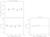 |
Fig. A.1 Magnitude measurements for SDSS J102915+172927 from Asiago and La Palma. On the left column are shown the Asiago Schmidt telescope measurements versus time (in hours) for the night of 5 May 2011. Top panel, the 4 V magnitude compared to a linear combination of the SDSS g and r magnitudes. Bottom panel, the 4 R magnitude measurements calibrated vs. the SDSS r band. In both panels the respective SDSS magnitudes are shown as short dashed lines and 1σ errors (long-dashed lines). On the right column are shown the r band measurements of the WFC/INT on La Palma for the night of 10 March 2003. |
A.2. INT La Palma
Only four images in the r band are present in the INT archive of images for the Wide Field camera (WFC). These images are part of the WFSur7, a collection of several programmes aiming at providing a quick coverage of the northern sky either in single- or multi-band. The PI of the observing programme is N. Walton, and to our knowledge the final catalogue and images have not yet been released but only intermediate products. The area surrounding our star was imaged on the night of 10 March 2003 with four images in the r band of 1 min each. We bias- and flat-field corrected the images using material from the same night and produced a DAOPHOT photometry of only the CCD where the star is present (CCD No. 3). We then calibrated the raw WFC photometry using the SDSS photometry of all stars in the field, properly excluding saturated and faint stars. The results are shown in the right column of Fig. A.1 in which we show the variation of the magnitude in time. The plot shows the reference SDSS r-band magnitude as listed in Table1. The scatter of the measurements is ≃ 0.007 mag with a 0.000 mag difference with the SDSS value.
With the material at our disposal we can safely conclude that there is an absence of long-term photometric variations at the level of Δr ≤ 0.006 variations considering the errors of the star. For the short term the variations seems to be insignificant. A longer-time monitoring with a better timing is underway to confirm this overall trend, considering that the monitoring covered less than 1 h of data-points for the Asiago Schmidt and 12 min for INT data.
Appendix B: Atomic data line-by-line
Lines analysed in this work.
All Tables
Non-LTE abundance corrections (dex) for the lines in SDSS J102915+172927 depending on surface gravity.
All Figures
|
Fig. 1 Mean temperature structure as a function of Rosseland optical depth of the CO5BOLD model used in this work (Teff = 5850 K, log g = 4.0, [Fe/H ] = −4.0; thick [blue] line), and of the 3D model used in Caffau et al. (2011c) (5850/4.0/ − 3.0; thin [red] line). For each model, the mean temperature is obtained by averaging the temperature as |
| In the text | |
|
Fig. 2 Best solutions of the fitted isochrones to the eight-band SDSS-2MASS photometry of SDSS J102915+172927. In the upper panel we depict the solution residuals. |
| In the text | |
|
Fig. 3 Measurement of the proper motion in the two coordinates, RA in the bottom panel, Dec in the upper panel. The zero points for the offsets are given by the position in the SDSS-DR7 catalogue. The results of the two different fits are shown: for all positions (long dashed line) and for the positions since 1990 only (dotted line). |
| In the text | |
|
Fig. 4 Galactic orbit for star J102915.14+172927.9 obtained using the PPMXL proper motion. The top-left panel shows the X/Z plane; top-right shows the Y/Z plane; bottom-left shows the X/Y plane; bottom-right shows the meridional plane R/Z. |
| In the text | |
|
Fig. 5 Range of the Ca ii H and K lines. From top to bottom, SDSS, X-Shooter, and UVES spectrum (solid black), overimposed the synthetic profile with metallicity –4.5, α-enhanced by 0.4 dex (solid green). |
| In the text | |
|
Fig. 6 G-band range of the the star SDSS J102915+172927: the observed spectrum (solid black) is compared to the known C-enhanced star HE 1327-2326. A zoom on the G-band is shown (solid black) compared to the best fit of the range (solid red) and with a synthetic profile enhanced in C by 2 dex (solid green). |
| In the text | |
|
Fig. 7 NH-band range of the the star SDSS J102915+172927: the observed spectrum (solid black) is compared to the best fit of the range (solid green) and with a synthetic profile enhanced in N by 2 dex (solid green). For comparison the known N-enhanced star HE 1327-2326 is shown. |
| In the text | |
|
Fig. 8 Emerging fluxes calculated using the 5811/4/−4.5 (solid black) and 5780/4.44/0 (dotted violet) model. Bold marks indicate the thresholds of the Fe i levels with excitation energy of 0.9 to 3.7 eV. |
| In the text | |
|
Fig. 9 Departure coefficients b, for the selected levels of the investigated atoms as a function of log τ5000 in the model atmosphere 5811/4.0/−4.5. Bottom panel: we show every fifth of the first 60 levels for Fe i. They are quoted in the bottom-right part of the panel. All remaining higher levels of Fe i are plotted by dotted curves. We show the same for Fe ii. They are quoted in the top-right part of the panel. SH = 0.1 throughout. |
| In the text | |
|
Fig. 10 Non-LTE abundance corrections for the Fe i lines in the 5811/4.0/–4.5 model depending on Eexc from the calculations with SH = 0.1 (filled circles) and SH = 1 (triangles). |
| In the text | |
|
Fig. 11 IS lines of Na i in the spectrum of SDSS J102915+172927. A telluric absorption line is denoted by a crossed circle. The solid line is a synthesis of the IS one-component model. |
| In the text | |
|
Fig. A.1 Magnitude measurements for SDSS J102915+172927 from Asiago and La Palma. On the left column are shown the Asiago Schmidt telescope measurements versus time (in hours) for the night of 5 May 2011. Top panel, the 4 V magnitude compared to a linear combination of the SDSS g and r magnitudes. Bottom panel, the 4 R magnitude measurements calibrated vs. the SDSS r band. In both panels the respective SDSS magnitudes are shown as short dashed lines and 1σ errors (long-dashed lines). On the right column are shown the r band measurements of the WFC/INT on La Palma for the night of 10 March 2003. |
| In the text | |
Current usage metrics show cumulative count of Article Views (full-text article views including HTML views, PDF and ePub downloads, according to the available data) and Abstracts Views on Vision4Press platform.
Data correspond to usage on the plateform after 2015. The current usage metrics is available 48-96 hours after online publication and is updated daily on week days.
Initial download of the metrics may take a while.