| Issue |
A&A
Volume 691, November 2024
|
|
|---|---|---|
| Article Number | A245 | |
| Number of page(s) | 10 | |
| Section | Galactic structure, stellar clusters and populations | |
| DOI | https://doi.org/10.1051/0004-6361/202452079 | |
| Published online | 15 November 2024 | |
SDSS J102915.14+172927.9: Revisiting the chemical pattern★
1
GEPI, Observatoire de Paris, Université PSL, CNRS,
5 Place Jules Janssen,
92190
Meudon,
France
2
INAF – Osservatorio Astronomico di Trieste,
Via G.B. Tiepolo 11,
34143
Trieste,
Italy
3
Universidad Andres Bello, Facultad de Ciencias Exactas, Departamento de Ciencias Físicas – Instituto de Astrofísica, Autopista Concepción-Talcahuano,
7100
Talcahuano,
Chile
4
Leibniz-Institut für Astrophysik Potsdam,
An der Sternwarte 16,
14482
Potsdam,
Germany
5
European Southern Observatory,
Alonso de Cordova 3107,
Vitacura,
Santiago,
Chile
6
GEPI, Observatoire de Paris, Université PSL, CNRS,
77 Av. Denfert Rochereau,
75014
Paris,
France
7
UPJV, Université de Picardie Jules Verne,
33 rue St Leu,
80080
Amiens,
France
8
Landessternwarte – Zentrum für Astronomie der Universität Heidelberg,
Königstuhl 12,
69117
Heidelberg,
Germany
9
Institute of Fundamental Physics of the Universe,
Via Beirut 2,
34151
Trieste,
Italy
★★ Corresponding author; This email address is being protected from spambots. You need JavaScript enabled to view it.
Received:
1
September
2024
Accepted:
6
October
2024
Abstract
Context. The small- to intermediate-mass (M < 0.8 M⊙), most metal-poor stars that formed in the infancy of the Universe are still shining today in the sky. They are very rare, but their discovery and investigation brings new knowledge on the formation of the first stellar generations.
Aims. SDSS J102915.14+172927.9 is one of the most metal-poor star known to date. Since no carbon can be detected in its spectrum, a careful upper limit is important, both to classify this star and to distinguish it from the carbon-enhanced stars that represent the majority at these metallicities.
Methods. We undertook a new observational campaign to acquire high-resolution UVES spectra. The new spectra were combined with archival spectra in order to increase the signal-to-noise ratio. From the combined spectrum, we derived abundances for seven elements (Mg, Si, Ca, Ti, Fe, Ni, and a tentative Li) and five significant upper limits (C, Na, Al, Sr, and Ba).
Results. The star has a carbon abundance A(C) < 4.68 and therefore is not enhanced in carbon, at variance with the majority of the stars at this Fe regime, which typically show A(C) > 6.0. A feature compatible with the Li doublet at 670.7 nm is tentatively detected.
Conclusions. The upper limit on carbon implies Z < 1.915 × 10⁻⁶, more than 20 times lower than the most iron-poor star known. Therefore, the gas cloud out of which the star was formed did not cool via atomic lines but probably through dust. Fragmentation of the primordial cloud is another possibility for the formation of a star with a metallicity this low.
Key words: stars: abundances / stars: Population II / stars: Population III / Galaxy: abundances / Galaxy: evolution / Galaxy: formation
Based on observations made with UVES at VLT 286.D-5045 and 112.25F3.001.
© The Authors 2024
 Open Access article, published by EDP Sciences, under the terms of the Creative Commons Attribution License (https://creativecommons.org/licenses/by/4.0), which permits unrestricted use, distribution, and reproduction in any medium, provided the original work is properly cited.
This article is published in open access under the Subscribe to Open model. This email address is being protected from spambots. You need JavaScript enabled to view it. to support open access publication.
1 Introduction
The process of formation of the first generation of stars (Pop III), formed after the Big Bang, is still not clearly understood and remains to be identified (see Bromm 2013). One of the main questions is whether low-mass stars can form from the primordial material, composed of isotopes of H, He, and traces of Li. A star of mass M ≈ 0.8 M⊙ or lower that formed in the first 100 Myr after the Big Bang would still be shining today on the main sequence. The fact that, to date, such a star has not been observed could serve as an argument against the formation of such primordial stars, yet the absence of evidence is not evidence of absence. Theoretically, the difficulty of forming a low-mass star from primordial matter is due to the lack of an efficient cooling mechanism that allows the star-forming gas cloud to continue to collapse instead of being stopped by the increasing radiative pressure caused by the consequential heating from compression. A star of large mass can be formed, since the gas cloud’s gravity is strong enough to overcome the pressure resulting from this heating (see Klessen & Glover 2023, and references therein).
Greif et al. (2010) showed that fragmentation of a large gas cloud can even take place for a primordial chemical composition resulting in the formation of low-mass primordial stars. However, the simulation could not be run long enough to be sure that the fragments will not merge again giving rise to a single massive star. Bromm & Loeb (2003) showed that if there is a small amount of C and O in the gas, the cooling goes through collisional excitation and radiative de-excitation. This led Frebel et al. (2007) to introduce the transition discriminant D = log[l0[C/H] + 0.3 × 10[O/H]]. The stars formed through atomic line cooling are characterised by D ≥ Dcrit ≃ −3.5 ± 0.2. The presence of carbon and oxygen in a primordial gas cloud provides a means of cooling the contracting gas to allow the formation of low-mass stars. But there is another way to cool at a chemical composition close to the pristine one. Schneider et al. (2012) proposed dust as a cooling mechanism for the formation of a second generation of low-mass stars. Smith et al. (2015) investigated the formation of the transition between Pop III and Pop II stars, suggesting that multiple scenarios probably contributed to this transition.
The star SDSS J102915.14+172927.9 (also known as Gaia DR3 3890626773968983296, hereafter SDSSJ102915+ 172927) was first studied by Caffau et al. (2011a) who claimed, based on UVES spectra, a very low iron abundance, [Fe/H] = −4.73, and a very low carbon abundance upper limit, A(C) ≤ 4.7. These authors found that the transition discriminant in this star is below the critical value defined above, thus invoking the cooling through dust (Omukai et al. 2005) to explain the formation of this star. The formation of SDSS J102915+172927 was theoretically investigated by several authors, and the conclusion was that the cooling was due to dust (see Schneider et al. 2012; Klessen et al. 2012; Chiaki et al. 2014; Bovino et al. 2016). Caffau et al. (2011a) claimed that this star was the most metal-poor object known in the Universe, with Z < 1.5 × 10⁻⁵, at the time of writing. Hattori et al. (2014) later suggested that SDSS J102915+172927 was formed from a primordial gas by zero-metal cooling, that is only through Lyα and H2 cooling (Silk 1977), and was later chemically enriched by accreting supernovae ejecta.
Clearly at the time of the discovery of SDSS J102915+172927, there was no way to derive an accurate surface gravity; the photometry available was consistent not only for a star on the main sequence, but also for a turn-off or sub-giant branch star. Caffau et al. (2011a) adopted an intermediate gravity of 4.0 dex, corresponding to the turn-off solution. MacDonald et al. (2013) claimed that the star is more likely to be a subgiant star. Their explanation for the low metal abundance of this star was that it is the result of ‘gravitational settling on the main sequence followed by incomplete convective dredge-up during subgiant evolution’. In this scenario, the fact that Fe is enhanced with respect to C implied that it was formed in an environment enriched by Type la supernova ejecta rich in Fe. With the advent of Gaia, the parallax put the star on the main sequence (see Bonifacio et al. 2018). Furthermore, the investigation of Ca ionisation conducted by Sitnova et al. (2019), which took into account the effects due to departures from the local thermodynamical equilibrium (LTE), that is so-called non-LTE (NLTE) effects. This ruled out the MacDonald et al. (2013) scenario.
Recently, a more sophisticated analysis of the same UVES data used in Caffau et al. (2011a), by Lagae et al. (2023), using a 3D stellar model and a NLTE treatment of the line formation for some elements, claimed that these new assumptions implied that the star was not as iron poor as was suggested in Caffau et al. (2012) in 1D-NLTE. Furthermore, Lagae et al. (2023) derived a much higher upper limit on C (A(C) < 5.39, the upper limit assuming a 1D model and local thermodynamical equilibrium (1D-LTE) is added with the uncertainty assigned by the authors), making the star’s transition discriminant compatible with its formation through atomic line cooling.
Since the carbon abundance determination is crucial to understanding whether the star formed through line cooling or dust cooling, we analysed newly observed high-resolution spectra that we combined with the previous observations. This allowed us to improve the signal-to-noise ratio (S/N) and to improve our estimates of the upper limits of several elements, including carbon.
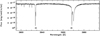 |
Fig. 1 Combined observed spectrum flux calibrated in the wavelength range of Ca II-K and -H. The two interstellar components are labelled as IS. The H line and few metallic lines (Fe I) are visible. |
2 Observations
For this investigation, we used the UVES spectra observed in the DDT programme 286.D-5045 of 2011 (7 h observations) and the specifically requested spectra observed during programme 112.25F3.001 (22 h observations). In programme 112.25F3.001, we observed in the setting DIC2 437+760 (wavelength ranges 373–499 and 565–946 nm), with slit 1.″4 (resolving power of 40000). We reduced all the spectra with the ESO pipeline (on gasgano version), the option of absolute flux calibration and, for the blue-arm spectra, we used the option ‘noappend’ in such a way as to keep all the orders separated. We corrected all the spectra for the barycentric velocity and derived the radial velocity for each observation. We shifted each spectrum for its radial velocity and merged the orders, as done for the ESPaDOnS spectra in Lombardo et al. (2021). We averaged all the spectra, and the spectrum obtained was used to derive the abundances (see Fig. 1).
A crucial point in the analysis of the G-band to derive the carbon abundance is the order merging of the UVES spectra. In the data reduction, we flux-calibrated the spectra, using the instrument response function derived from the observation of spectrophotometric standard stars1. As a test, from the UVES spectra we extracted the two orders where the CH molecules are the strongest in the G-band, corresponding to wavelength range 429–433 nm, that is order 108 and 109. We added all the spectra from prog. 1D 286.D-5045 and 112.25F3.001, separately. We averaged the two added spectra. We then used the Gaia-XP spectrum as the flux for the star, by scaling the UVES spectra on the Gaia-XP (Gaia Collaboration 2023a). This step corrects for any flux lost at the slit during the observation. We merged the two spectra extracted from the two orders. We rebinned the Gaia-XP spectrum on the UVES spectra and then divided the two. The obtained spectrum is the normalised one that we compared to the complete merge spectrum, selected and normalised in the G-band wavelength range. The two spectra are indiscernible, so we decided to use the complete merged spectrum for all the chemical investigations. We underline that the overlap between order 109 and 108 is in the range 429.5–430.5 nm, which is where there are some of the strongest CH lines.
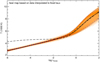 |
Fig. 2 Three-dimensional versus 1D temperature structure for stellar parameters Teff=5773 K, log ɡ=4.7, and metallicity [M/H]=−4.0. The orange band outlines the 3D temperature distribution of the high-resolution model resampled to 70 × 70 × 160 grid points. The width of the temperature distribution encountered on surfaces of equal Rosse-land optical depth is indicated by the dashed blue lines enclosing 95.5% of the data points at each height. The solid black line shows the average temperature of the 3D model, the long-dashed black line represents the T(τRoss) relation predicted by a 1D model atmosphere with identical stellar parameters, treating convection by standard mixing-length theory, but otherwise using the same input physics as the 3D hydrodynamical model. |
3 Model atmospheres
We computed an ATLAS 12 model (Kurucz 2005) with the stellar parameters discussed in Sect. 4.2 and abundances derived by Caffau et al. (2012). This model has been used to derive the chemical abundances and the upper limits in the present work.
We also computed two dedicated 3D hydrodynamical model atmospheres with the latest version of the C05BOLD code (see Freytag et al. 2012, plus updates) for stellar parameters that closely represent this star (Teff=5773 K, log ɡ=4.7, [M/H]=−4.0, see Sect. 4.2). The low-resolution model has 140 × 140 × 160 grid cells, and the high-resolution models covers the same volume by 280 × 280 × 160 cells. The frequency dependence of the radiative opacity is represented by 11 bins, each comprising opacities of similar strength. Figure 2 depicts the temperature stratification of the resampled high-resolution model, which is almost identical to that of its low-resolution counterpart.
As is well known, the temperature stratification of the photospheres of metal-poor stars is sensitive to hydrodynamical flows that cannot be modelled in 1D. This implies a systematic photospheric temperature difference between standard 1D model atmospheres where convection is treated by the mixing-length theory and 3D hydrodynamical simulations where convective overshoot is emerging naturally. For the stellar parameters considered here, the temperature of the 3D model is cooler than predicted by the corresponding 1D model for optical depths log τRoss < −2.0, whereas the temperature difference is reversed in the range −2.0 < log τRoss < −0.5 (compare solid and dashed lines in Fig. 2). It is noteworthy that the amplitude of the temperature fluctuations in the upper photosphere is remarkably small; the 3D model can probably be represented reasonably well by its (3D) mean structure. However, we make use of the full 3D results in this work. The low amplitude of the photospheric temperature fluctuations was already recognised in the 3D model for the star used by Caffau et al. (2012) and tentatively traced back to the damping influence of an increased specific heat caused by H2 molecular formation. Thygesen et al. (2017, see their Fig. 1) show that small temperature fluctuations are a common property of metal-poor 3D models in the considered regime of effective temperatures and surface gravity.
As mentioned above, all chemical abundance determinations in this work (including the upper limit estimates) are based on ATLAS 12 state-of-the-art 1D model atmospheres together with the line formation code SYNTHE (Kurucz 2005), used to compute synthetic spectra from the ATLAS 12 models. In the case of carbon only, we consider the 3D correction described in Sect. 4.5, resulting in a significantly lower C abundance.
4 Analysis
4.1 Radial velocity
We derived the radial velocity from all the spectra, already corrected for the barycentric velocity with template matching. We compared each observed spectrum with a synthetic one. We find 〈Vr〉 = −34.9 ± 0.6 km s−1, which is compatible with no radial velocity variation from the UVES spectra. We shifted each spectrum for the derived radial velocity before adding them, because slightly different radial velocity values can be due to the centring of the star on the slit.
4.2 Stellar parameters
We derived the stellar parameters using the Gaia DR3 (Gaia Collaboration 2023b) photometry and parallax. As in Lombardo et al. (2021), we compared the GBP – GRP Gaia colour to a grid of synthetic colours to derive the effective temperature, Teff. Once the Teff was obtained, we derived the gravity from the Gaia parallax, corrected by the zero-point as suggested by Lindegren et al. (2021), using the Stefan-Boltzmann equation. For the mass, we compared the stellar parameters to MIST (Dotter 2016; Choi et al. 2016), BASTI (Hidalgo et al. 2018; Pietrinferni et al. 2021), and Chieffi FRANEC isochrones (Chieffi, priv. comm.) and converged to 0.65 M⊙. This is in perfect agreement with the masses (0.62 M⊙ to 0.70 M⊙) reported in Table 2 by Caffau et al. (2012). If the corrections were not applied to the zero-point of the parallax, the gravity would become 0.05 dex higher and the temperature 6 K cooler. This would lead to negligible changes in the abundances.
The extinction we adopted was AV = 0.08 (Rosine Lallement, priv. comm.), and at each step we interpolated the extinction coefficient in a grid of synthetic coefficients. Assuming a metallicity of −4.7 for the first iteration, we derived the initial estimate of the stellar parameters and from them the metallicity. The final stellar parameters we adopted to compute the ATLAS 12 model were: Teff=5780 K, log ɡ=4.60, no α-enhancement, and a microturbulence (ξ) of 1 km s−1. The conclusion on the absence of α-enhancement is based on Mg and Ca. The microturbulence is assumed, as there are not enough Fe I lines with various line strengths to derive it.
The Fe I lines used to derive the metallicity are all in a limited lower energy range (Elow < 1.61 eV), making them not useful for deriving Teff from a null-trend of A(Fe) with Elow. If we group the Fe I lines in three sets of energy range, we obtain [Fe/H] = −4.64 from lines in the range 0–0.85 eV, [Fe/H] = −4.77 for lines in the range 0.85–1.02 eV, and [Fe/H] = −4.78 for lines in the range 1.4–1.61 eV. Among the two sets of highest Elow, there is no trend, as in Cayrel et al. (2004), while the lines in the set with the lowest energy provide, on average, a higher A(Fe) (as in Cayrel et al. 2004).
4.3 Kinematics
In order to evaluate the kinematic properties of SDSS J102915+172927, we used the same techniques presented in Bonifacio et al. (2024) and Caffau et al. (2024). In particular, we used the Gaia DR3 (Gaia Collaboration 2023b) coordinates, parallax, and proper motions, and the radial velocity we measured from our spectra, as input to the Galpy code (Bovy 2015). The parallax was corrected for the zero-point following Lindegren et al. (2021). We adopted the standard Milky Way potential MWPotential2014, the solar peculiar motions by Schönrich et al. (2010), a distance of the Sun from the Galactic centre of 8 kpc, and a circular velocity at the solar distance of 220 km s−1 (Bovy et al. 2012). The stellar orbit was back-integrated for 1 Gyr. We estimated the errors on the calculated quantities as the standard deviation of the values obtained, repeating the calculations with a 1000 random realisations of the input parameters. We used the pyia code (Price-Whelan 2018) to perform the extractions from a multivariate Gaussian, which adopts the errors in the input parameters as standard deviations and takes into account the correlation between the input parameters.
Figure 3 shows the SDSS J102915+172927 orbit in X, Y, and Z rectangular Galactocentric coordinates (bottom-left, bottom-right and upper-left panels). The current position of the star is indicated as a black solid star. SDSS J102915+172927 lies at a distance of 1.47 ± 0.13 kpc from the Sun and of 8.72±0.07kpc from the Galactic centre, 1.24 ± 0.11 kpc above the Galactic plane. Its orbit is pro-grade, confined within Zmax = 2.42 ± 0.26 kpc of the Galactic plane and of low eccentricity (e = 0.02 ± 0.01), with peri- and apo-Galactocentric distances of rperi = 8.64 ± 0.05 kpc and rap = 8.93 ± 0.09 kpc. The upper-right panel shows the SDSS J102915+172927 position in the Toomre diagram, namely the transversal velocity component, versus a combination of the radial and vertical velocity components in Galactocentric cylindrical coordinates. We plotted for reference, the ‘good parallax sub-sample’ of Bonifacio et al. (2021), where stars are classified as belonging to the thin disc (red), thick disc (green), and halo (blue), according to the scheme adopted by Bensby et al. (2014). SDSS J102915+172927 is classified as a ‘thick disc’ star according to this scheme.
The kinematics of SDSS J102915+172927 have also been previously investigated by Sestito et al. (2019), Di Matteo et al. (2020) and Dovgal et al. (2024). In particular, Dovgal et al. (2024) followed the same methodology as Sestito et al. (2019) but used Gaia DR3 astrometric parameters. Di Matteo et al. (2020) inverted the Gaia DR2 parallax corrected by a zero-point of −0.03 to derive the distance (1.31 kpc), while Dovgal et al. (2024) inferred a distance from the Sun of 1.49 ± 0.32 kpc.
Our results are in good agreement with both analyses. Dovgal et al. (2024) indicate that the star is on a pro-grade, almost circular (e = 0.09 ± 0.02) disc orbit around the Galactic centre, confined to Zmax = 2.36 ± 0.60 kpc of the Galactic plane. Similarly to us, these authors used the galpy code and the MWPotential2014 potential, which, however, they modified to have a more massive dark matter halo. Di Matteo et al. (2020), who used different codes and Galactic potential, also obtain for this star a quasi-circular orbit (e = 0.04, rperi = 8.9 ± 0.0 kpc and rap = 9.6 ± 0.2 kpc), confined close to the Galactic plane (Zmax = 2.2 kpc).
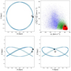 |
Fig. 3 Orbit of SDSS J102915+172927 in the Y vs. X (upper-left), Z vs. X (bottom-left), and Z vs. Y (bottom-right) planes. X, Y, and Z are Galactocentric Cartesian coordinates. Upper-right panel: |

4.4 Abundances
To derive the abundances, we used MyGIsFOS (Sbordone et al. 2014) but in a non-standard way. We computed an ATLAS 12 model (Kurucz 2005) with the abundances derived by Caffau et al. (2012). With SYNTHE (Kurucz 2005), using the ATLAS 12 model (thus, keeping the same temperature structure), we computed a grid of synthetic spectra varying in steps of 0.2 dex in abundance for all elements. We built a grid with these syntheses, to be used by MyGIsFOS. We selected the ranges with no lines to be used to pseudo-normalise the observed spectrum and in the same way the synthetic spectra. We verified that the ranges to be used to pseudo-normalise the spectra were clean from unexpected emission or absorption (e.g. telluric lines), and we verified all fits. We derived abundances for six elements (see Table 1). As expected, the abundances derived are in agreement with Caffau et al. (2011a, 2012). Due to the high quality of the spectrum, the Fe abundance is now based on 56 Fe I features, and not 43 as was the case in Caffau et al. (2012). We derived [Fe/H] = −4.73 ± 0.09 dex. For the lD-NLTE correction on iron, Caffau et al. (2012) derived +0.13 dex from three Fe I lines. This value is in agreement with +0.12 dex derived from 32 Fel lines when using the corrections from Bergemann et al. (2012). The differences with other lD-NLTE corrections for Fe I in this star found in the literature are rooted in the different assumptions made to take into account the collisions with hydrogen atoms. The lD-NLTE correction of +0.25 dex derived by Lagae et al. (2023) is in agreement with the NLTE correction of +0.24 dex (Caffau et al. 2012) adopting SH = 0.1. Ezzeddine et al. (2017) derived a NLTE correction for Fe of +0.4 dex using their semi-empirical quantum fitting method (Ezzeddine et al. 2018) to estimate the effect of collisions with hydrogen atoms. We adopt the value computed by Caffau et al. (2012) for the NLTE correction on Fe with SH = 1, a choice that was carefully taken at the time. In addition, we favour a smaller NLTE correction in Fe because there are some extremely metal-poor stars that are not enhanced or slightly poor in α elements (see e.g. Caffau et al. 2013), but very few are poor in α elements (see Li et al. 2022). Increasing the Fe abundance would make this star α–poor.
Here we did not use the Mg i-b lines used by Caffau et al. (2012) because only the 2011 observations cover this wavelength range and the S/N is low. Instead, we used only the UV lines that with combined spectra provide a high S/N of 78. From the three Mgl lines (382.9, 383.2 and 383.8 nm), we derived [Mg/H] = −4.67 ± 0.04. The agreement with Caffau et al. (2012) is good ([Mg/H] = −4.73 from these three lines). For the Mg I lines used here, Caffau et al. (2012) has a NLTE correction of +0.13 dex, which is in agreement with +0.17 derived by using the corrections from Bergemann et al. (2017) and with the value in Lagae et al. (2023).
For the Si I line at 390.5 nm, already investigated in Caffau et al. (2012), we derived a lower Si abundance ([Si/H] = −4.37), but we have a better quality spectrum (S/N=84). The NLTE correction in Caffau et al. (2012) is +0.35 dex for the dwarf solution, the value that we adopt here. From the 422 nm Ca I line, we derived [Ca/H] = −4.76. A NLTE correction of +0.24 was derived by Caffau et al. (2012) for the dwarf solution. For Ti we investigated only the Ti II line at 336.1 nm. According to Sitnova et al. (2016), Ti ionised lines form close to the LTE condition. We kept five Ni I lines and derived [Ni/H] = −4.64 ± 0.15.
We derived significant upper limits for Na, and the star is found to be poor in Na (see Fig. 4). We estimated S/N=85 in the wavelength range of the strongest Na I D1 line at 588.9nm. By using Cayrel’s formula (see Cayrel 1988), we derived the minimum equivalent width (EW) detectable. We multiplied this value by a factor of three and derived the abundance by interpolating in a curve of growth. The observed spectrum compared to the synthesis highlighting the upper limit is shown in Fig. 4. We also derived a significant upper limit for Al using the same technique used to determine Na (with S/N=85, see Fig. 5). By investigating the 407 nm Sr II line (S/N=90), and proceeding as for Na and Al, we concluded that the star is surely under-abundant in Sr (see Fig. 6). With the NLTE correction of 0.14 dex for Sr derived by Caffau et al. (2012), the star is still poor in heavy elements, as is frequently the case in extremely metal-poor stars (see François et al. 2007). For Ba (S/N=130), the upper limit is less stringent (see Fig. 7) indicating that the star is compatible with being slightly enhanced in Ba. The abundances, the upper limits and the NLTE corrections adopted are reported in Table 1.
We do not clearly see the Li I doublet at 670.7 nm. Using Cayreľs formula (see Cayrel 1988, S/N=150), we derived A (Li) < 0.88 at 3σ and A (Li) < 1.08 at 5σ. However, there was a hint of a feature slightly exceeding the noise level. We smoothed the spectrum to increase the S/N per pixel, but the feature did not appear clearly as the Li doublet, nor did it disappear. We looked at the spectra individually to see if the hint corresponds to a specific observation, but this feature builds up by adding the observations. We conclude that there is a tentative but very uncertain Li detection at A(Li) ~ 1.08. The detection is very uncertain because the feature at 670.8 nm has a different shape than the synthesis (see Fig. 8 for the comparison of the observed with synthetic spectra).
A fundamental point for this star is the carbon abundance, in order to confirm whether or not the star is carbon normal, i.e. not a carbon-enhanced metal-poor (CEMP) star. However, nitrogen is also important to derive. Neither С from the G-band nor N from the NH band are visible in the observed spectrum. Since the NH band at 336 nm is expected to be much weaker than the CH lines in the G-band, and no new data is available at 336 nm, we concentrated on the determination of an upper limit for C. We fit the NH band, by which we mean that we fit the noise in the region with syntheses based on the new stellar parameters, which led to weaker synthetic features. By using the line-list from Fernando et al. (2018) we derived from the fit: A(N) = 4.42 ± 0.15. We therefore conclude that A(N) < 4.87, which is the results of the fit added by 3σ, and it is higher than the value in Caffau et al. (2012) because of the higher surface gravity now adopted.
Abundances derived for SDSS J102915+172927.
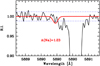 |
Fig. 4 Observed spectrum (solid black) in the wavelength of the Na I D1 line compared to a synthesis (solid red) with A(Na) derived from Cayrel’s formula multiplied by a factor 3. The S/N of 85 is highlighted by the dashed blue lines. |
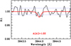 |
Fig. 5 Observed spectrum (solid black) in the wavelength of the 349.9 nm A1 I line compared to a synthesis (solid red) with A(Al) from the upper limit. The S/N of 85 is highlighted by the dashed blue lines. |
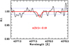 |
Fig. 6 Observed spectrum (solid black) in the wavelength of the 407.7 nm Sr II line compared to a synthesis (solid red) with A(Sr) from the upper limit. The S/N of 90 ratio is highlighted by the dashed blue lines. |
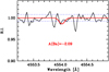 |
Fig. 7 Observed spectrum (solid black) in the wavelength of the 455.4 nm Ba II line compared to a synthesis (solid red) with A(Ba) from the upper limit. The S/N of 130 is highlighted by the dashed blue lines. |
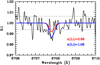 |
Fig. 8 Observed spectra (solid black) in the wavelength of the 670.7 nm Li I doublet compared to synthesis (solid red and blue). The 1σ S/N is highlighted by the dashed blue lines. |
4.5 Carbon abundance
We computed synthetic profiles with SYNTHE using the ATLAS 12 model computed for the star. We fit the G-band by choosing the wavelength ranges hosting the strongest CH transitions. The molecular data of the CH lines are from Masseron et al. (2014). We fit a metallic line (a Fe I line is present in the wavelength range) with the CH features. We adjusted A(Fe) in the computation of the synthesis to fit the line as well as possible. This was done in order to float the shift in wavelength to this strong and well-defined line. We believe that in this spectral range, besides the Fe I line, there is only noise, corresponding to S/N ~ 100, compatible with a weak G-band. Fitting ranges in the G-band including an atomic line and the strongest CH features, we derived values in the range: 3.60 < A(C) < 4.23. In the wavelength range around 432 nm, from the fit we derived a very low carbon value (A(C) = 3.60), making the star poor in C, in line with the α-elements. In the wavelength range around 429 nm and 430 nm, we find A(C) = 4.23, consistent with the results by Spite et al. (2005) in a sample of unmixed stars at a metal-poor regime (−4.2 < [Fe/H] < −2). In Fig. 9, the fits are shown. From the fit in the G-band, we deduced that A(C) < 4.71, which is the higher result from the fit added by 3σ of its uncertainty, which implies [C/H] < −3.79 and [C/Fe] < 0.94.
As for the other elements for which we derived an upper limit, we selected the strongest CH features in the G-band, computed the EW at 3σ according to Cayrel’s formula and interpolated in a computed curve of growth. The results are shown in Fig. 10, and the upper limit we derived at 3σ is A(C) < 4.68, which provides [C/H] < −3.82 and [C/Fe] < 0.91 with the 1D-LTE Fe value from Table 1. If we apply the NLTE correction on Fe, we derive [C/Fe] < 0.79.
The upper limits that we derived for carbon are generally lower than the ones provided by Lagae et al. (2023). This is due to (1) the improved S/N of our observed spectrum in the region of the G-band, which doubled with the new observations, and (2) a different methodology that we followed: while Lagae and collaborators consider a χ2 between synthesis and observation computed over a wider wavelength range, we focused on localised strong CH features that have the chance to stand out of the noise.
The 3D versus ID temperature differences (see Fig. 2) are expected to have consequences for the spectral line formation and hence for the abundances derived from the two types of model atmospheres. The strongest CH lines in the G-band, for example, form over a wide range of optical depth, centred on log τRoss ≈ −4, as demonstrated by the relevant contribution functions shown in Fig. 11. For a given carbon abundance, the 3D models will therefore predict stronger CH lines than the corresponding ID model.
For a quantitative determination of the 3D effects on the CH lines in the G-band, we computed synthetic spectral line profiles with the Linfor3D line formation code (Steffen et al. 2024) from (i) the 3D model and (ii) a reference ID model atmosphere with identical stellar parameters and using the same opacity tables as the 3D model. Figure 12 shows the 3D and ID synthetic profiles of the CH feature at λ 4293 Å, for a given carbon abundance of A(C)=4.75. The comparison clearly demonstrates that the 3D lines are significantly stronger than in the ID case. Quantitatively, the carbon abundance deduced by means of a 3D analysis of a typical CH feature in the G-band is about 0.5 dex lower than the standard ID result. This was explored in detail in Gallagher et al. (2016). The magnitude of this 3D correction is found to be independent of the spatial resolution of the 3D model. From the strongest three CH features used to derive the A(C) upper limit, we derived an average 3D correction of −0.53 (with A(C)=4.5). The value increases with increasing A(C) abundance (it is −0.72 in the case of A(C)=5.75). By applying the 3D correction on the С upper limit, we derived [C/Fe] < 0.26.
NLTE calculations for CH have only recently been conducted for a limited number of stellar parameter combinations by Popa et al. (2023). They find, in the most extreme case of a metal-poor giant, a NLTE correction of +0.2 dex. We consider this an upper limit of a possible NLTE correction to be present here, since SDSSJ102915+172927 is a dwarf where collisions play a more pronounced role, thus driving the system towards LTE. In addition, Deshmukh & Ludwig (2023) find negligible deviations from chemical equilibrium of CH in the photospheres of metal-poor turn-off stars. The higher gravity and slightly lower effective temperature of SDSS J102915+172927 suggest that it is unlikely that chemical equilibrium comes out differently in comparison to the situation at the turn-off. Hence, it appears rather unlikely that departures from LTE or chemical equilibrium alter the overall picture described before qualitatively.
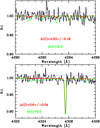 |
Fig. 9 Observed spectra (solid black) in the wavelength of the G-band compared to the best fit (solid red) and a synthesis (solid green) to visualise the strongest CH features. The S/N is highlighted by the dashed blue lines. The visible strong line is Fe I. |
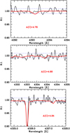 |
Fig. 10 Observed spectra (solid black) in the wavelength of the G-band compared to the synthesis with 3σ (solid red) abundance in the correspondence of the three strongest feature in the G-band. The S/N is highlighted by the dashed blue lines. |
 |
Fig. 11 EW contribution function, dW/d log τRoss for three of the strongest CH features in the G-band, located at 4293 Å (dashed), 4303 Å (solid), and 4327 A (dash-dotted), respectively, as computed from the 3D model shown in Fig. 2. The area under each curve gives the line’s EW in mÅ for the disk-integrated stellar spectrum. |
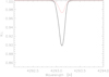 |
Fig. 12 Synthetic 3D profile (solid black, EW=l.57pm) compared to the ID synthesis (solid red, EW=0.44pm) of the CH feature at 429 nm in the case of A(C)=4.75. We note that the carbon feature is a blend of several components, such that it appears asymmetric even in the ID synthesis. |
5 Discussion and conclusions
To derive the upper limit on the metallicity, Z, of the star, we applied the abundances in Table 1 and the 3σ upper limits. For the elements for which we have no information, we applied the solar-scaled value, except for N and О for which we applied a value scaled with the С upper limit. We derived Z < 1.915×10⁻⁶ (Z < 1.252 × 10⁻⁴ Z⊙ with Z⊙ from Caffau et al. 2011b or Z < 1.378 × 10⁻⁴ Z⊙ with Z⊙ from Asplund et al. 2021). This value relies on the 1D-LTE abundances. The NLTE corrections would increase the metallicity, but only of the elements that represent a minority in the stellar photosphere: an increase by 0.5 dex in Fe would bring the Z upper limit to 1.970 × 10⁻⁶. However, if corrections have to be applied, the 3D corrections for С should be taken into account, reducing the stellar metallicity by a larger amount, because carbon is much more abundant in the stellar photosphere than iron. By applying the NLTE correction from Table 1 and the 3D correction on C, we derived Z < 1.660 × 10⁻⁶.
With the ID upper limit [C/H] < −3.82 and adopting the scaled value for oxygen, for this star, we derived D < −3.71. By applying the 3D correction on the С abundance and leaving the [O/H] upper limit unchanged, we derived D < −4.23. These values suggest that the star was formed through dust cooling, as suggested by several authors (see Schneider et al. 2012; Klessen et al. 2012; Chiaki et al. 2014; Bovino et al. 2016), but the fragmentation scenario presented by Greif et al. (2010) is also a possibility for the formation of this star.
SDSS J102915+172927 is a peculiar star for several reasons: (i) it is extremely low in metallicity (ii) with no enhancement in carbon; (iii) it is not enhanced in the α-elements, and (iv) it is hosted in a Galactic disc orbit.
Few stars with [Fe/H] < −4.5 dex are known, and just two stars (this star and Pristine J221.8781+09.7844 Starkenburg et al. 2018) do not have a measurable G-band, putting them outside the CEMP class that hosts all the other stars known in this iron-abundance range. SDSS J102915+172927 is, according to our analysis, the only star with [Fe/H] < −4.5 dex not satisfying the condition [C/Fe] > 1 dex proposed by Beers & Christlieb (2005) to define CEMP stars. Pristine J221.8781+09.7844 has a loose [C/Fe] upper limit (2.3 dex in Lardo et al. 2021, with S/N=90 at 400 nm), but the G-band is not visible in its spectrum either. The lower the [Fe/H] ratio, the more difficult is to reach a [C/Fe] < 1 dex upper limit, according to the definition of CEMP stars in Beers & Christlieb (2005). Looking at the ultra iron-poor stars in Bonifacio et al. (2015), the low carbon band is around A(C) ~ 6.7, such that A(C) < 5.5 could be a better definition for a star not belonging to the CEMP class in the case that it has [Fe/H] < −4.5.
SDSS J102915+172927 shows a feature at the wavelength of the 670.7 nm Li doublet. This is a tentative Li detection providing A(Li) = 1.08 (see Table 1), a value well below the Spite plateau (Spite & Spite 1982). In any case, whether with a low Li abundance or entirely free of Li, the star could have destroyed the Li during its life (e.g. if it were a blue straggler) or have formed from a gas cloud already depleted in Li. Also, HE 0107 5240 (Christlieb et al. 2002) has less lithium than expected from its parameters. In fact, A(Li) < 0.50 (see Aguado et al. 2022), and the star should still have A(Li) ~ 1 (Mucciarelli et al. 2022). This can be an indication that the ultra Fe-poor stars formed from a cloud depleted in Li. But, to add complexity to the picture, we recall that at the ultra Fe-poor regime, there are also stars with the Li abundance on the Spite plateau (e.g. SDSS J002314.00+030758.0, Aguado et al. 2019) or that were on the Spite plateau before diluting the Li following the first dredge-up (e.g. SMSS J031300.36-670839.3, Keller et al. 2014).
The relatively low contents of Al and Na are still compatible with extremely metal-poor (EMP) stars (see Cayrel et al. 2004). The stringent Sr upper limit puts the star as not rich in heavy elements but it is still consistent with the high-quality EMP sample investigated by François et al. (2007). The star is in a pro-grade disc orbit, confined in the Galactic disc. Due to the poor metal content of this star, Klessen & Glover (2023, see also references therein) suggest that it formed through dust cooling.
The two considerations, that (1) the star is in a Galactic disc orbit and (2) its photospheric metal content is low, may invite to consider SDSS J102915+172927 as a Pop III star, polluted by the interstellar gas during its long (probably more than 13 Gyr) journey through the Galaxy. Yoshii (1981) suggested that main-sequence stars accrete surface material through encounters with gas and that the effect is more evident for stars with low-eccentricity orbits, with amount of the accreted material depending on the dimension and obviously on the number of the encountered clouds. The number of encountered clouds is expected to be large due to the long life of this star and the higher number of gas clouds on the Galactic disc than on the Galactic halo; the relatively low [Mg/Fe] and [Ti/Fe] ratios in SDSS J102915+172927 are consistent with the pollution expected by Johnson (2015) in a main-sequence Pop III star in the case of ρgrain = 3 g cm−3, but, in this case, the expected [Si/Fe] would be expected to be lower by about 0.3 dex.
Our investigation confirms SDSS J102915+172927 to be the most metal poor object known to date and does not support any enhancement in carbon. This leaves open the routes of dust cooling or fragmentation to explain its formation.
Acknowledgements
We wish to thank Rosine Lallement for providing us the extinction for the star here investigated, and Cis Lagae for discussions on the determination of upper abundance limits. EC and PB acknowledge support from the ERC advanced grant no. 835087 – SPIAKID. This work has made use of data from the European Space Agency (ESA) mission Gaia (https://www.cosmos.esa.int/gaia), processed by the Gaia Data Processing and Analysis Consortium (DPAC, https://www.cosmos.esa.int/web/gaia/dpac/consortium). Funding for the DPAC has been provided by national institutions, in particular the institutions participating in the Gaia Multilateral Agreement. This research has made use of the SIMBAD database, operated at CDS, Strasbourg, France.
Appendix A Lines used
In Table A.1, the atomic lines investigated are listed.
Atomic data.
References
- Aguado, D. S., González Hernández, J. I., Allende Prieto, C., & Rebolo, R. 2019, ApJ, 874, L21 [NASA ADS] [CrossRef] [Google Scholar]
- Aguado, D. S., Molaro, P., Caffau, E., et al. 2022, A&A, 668, A86 [NASA ADS] [CrossRef] [EDP Sciences] [Google Scholar]
- Asplund, M., Amarsi, A. M., & Grevesse, N. 2021, A&A, 653, A141 [NASA ADS] [CrossRef] [EDP Sciences] [Google Scholar]
- Beers, T. C., & Christlieb, N. 2005, ARA&A, 43, 531 [NASA ADS] [CrossRef] [Google Scholar]
- Bensby, T., Feltzing, S., & Oey, M. S. 2014, A&A, 562, A71 [NASA ADS] [CrossRef] [EDP Sciences] [Google Scholar]
- Bergemann, M., Lind, K., Collet, R., Magic, Z., & Asplund, M. 2012, MNRAS, 427, 27 [Google Scholar]
- Bergemann, M., Collet, R., Amarsi, A. M., et al. 2017, ApJ, 847, 15 [NASA ADS] [CrossRef] [Google Scholar]
- Bonifacio, P., Caffau, E., Spite, M., et al. 2015, A&A, 579, A28 [NASA ADS] [CrossRef] [EDP Sciences] [Google Scholar]
- Bonifacio, P., Caffau, E., Spite, M., et al. 2018, RNAAS, 2, 19 [NASA ADS] [Google Scholar]
- Bonifacio, P., Monaco, L., Salvadori, S., et al. 2021, A&A, 651, A79 [NASA ADS] [CrossRef] [EDP Sciences] [Google Scholar]
- Bonifacio, P., Caffau, E., Monaco, L., et al. 2024, A&A, 684, A91 [NASA ADS] [CrossRef] [EDP Sciences] [Google Scholar]
- Bovino, S., Grassi, T., Schleicher, D. R. G., & Banerjee, R. 2016, ApJ, 832, 154 [NASA ADS] [CrossRef] [Google Scholar]
- Bovy, J. 2015, ApJS, 216, 29 [NASA ADS] [CrossRef] [Google Scholar]
- Bovy, J., Allende Prieto, C., Beers, T. C., et al. 2012, ApJ, 759, 131 [NASA ADS] [CrossRef] [Google Scholar]
- Bromm, V. 2013, Rep. Progr. Phys., 76, 112901 [CrossRef] [Google Scholar]
- Bromm, V., & Loeb, A. 2003, Nature, 425, 812 [NASA ADS] [CrossRef] [Google Scholar]
- Caffau, E., Bonifacio, P., François, P., et al. 2011a, Nature, 477, 67 [NASA ADS] [CrossRef] [Google Scholar]
- Caffau, E., Ludwig, H. G., Steffen, M., Freytag, B., & Bonifacio, P. 2011b, Sol. Phys., 268, 255 [Google Scholar]
- Caffau, E., Bonifacio, P., François, P., et al. 2012, A&A, 542, A51 [NASA ADS] [CrossRef] [EDP Sciences] [Google Scholar]
- Caffau, E., Bonifacio, P., François, P., et al. 2013, A&A, 560, A15 [NASA ADS] [CrossRef] [EDP Sciences] [Google Scholar]
- Caffau, E., Bonifacio, P., Monaco, L., et al. 2024, A&A, 684, L4 [NASA ADS] [CrossRef] [EDP Sciences] [Google Scholar]
- Cayrel, R. 1988, in The Impact of Very High S/N Spectroscopy on Stellar Physics, 132, eds. G. Cayrel de Strobel, & M. Spite, 345 [NASA ADS] [CrossRef] [Google Scholar]
- Cayrel, R., Depagne, E., Spite, M., et al. 2004, A&A, 416, 1117 [NASA ADS] [CrossRef] [EDP Sciences] [Google Scholar]
- Chiaki, G., Schneider, R., Nozawa, T., et al. 2014, MNRAS, 439, 3121 [NASA ADS] [CrossRef] [Google Scholar]
- Choi, J., Dotter, A., Conroy, C., et al. 2016, ApJ, 823, 102 [Google Scholar]
- Christlieb, N., Bessell, M. S., Beers, T. C., et al. 2002, Nature, 419, 904 [NASA ADS] [CrossRef] [PubMed] [Google Scholar]
- Deshmukh, S. A., & Ludwig, H. G. 2023, A&A, 675, A146 [NASA ADS] [CrossRef] [EDP Sciences] [Google Scholar]
- Di Matteo, P., Spite, M., Haywood, M., et al. 2020, A&A, 636, A115 [NASA ADS] [CrossRef] [EDP Sciences] [Google Scholar]
- Dotter, A. 2016, ApJS, 222, 8 [Google Scholar]
- Dovgal, A., Venn, K. A., Sestito, F., et al. 2024, MNRAS, 527, 7810 [Google Scholar]
- Ezzeddine, R., Frebel, A., & Plez, B. 2017, ApJ, 847, 142 [Google Scholar]
- Ezzeddine, R., Merle, T., Plez, B., et al. 2018, A&A, 618, A141 [NASA ADS] [CrossRef] [EDP Sciences] [Google Scholar]
- Fernando, A. M., Bernath, P. F., Hodges, J. N., & Masseron, T. 2018, J. Quant. Spec. Radiat. Transf., 217, 29 [NASA ADS] [CrossRef] [Google Scholar]
- François, P., Depagne, E., Hill, V., et al. 2007, A&A, 476, 935 [Google Scholar]
- Frebel, A., Johnson, J. L., & Bromm, V. 2007, MNRAS, 380, L40 [NASA ADS] [CrossRef] [Google Scholar]
- Freytag, B., Steffen, M., Ludwig, H. G., et al. 2012, J. Computat. Phys., 231, 919 [NASA ADS] [CrossRef] [Google Scholar]
- Gaia Collaboration (Montegriffo, P., et al.) 2023a, A&A, 674, A33 [CrossRef] [EDP Sciences] [Google Scholar]
- Gaia Collaboration (Vallenari, A., et al.) 2023b, A&A, 674, A1 [NASA ADS] [CrossRef] [EDP Sciences] [Google Scholar]
- Gallagher, A. J., Caffau, E., Bonifacio, P., et al. 2016, A&A, 593, A48 [NASA ADS] [CrossRef] [EDP Sciences] [Google Scholar]
- Greif, T. H., Glover, S. C. O., Bromm, V., & Klessen, R. S. 2010, ApJ, 716, 510 [NASA ADS] [CrossRef] [Google Scholar]
- Hattori, K., Yoshii, Y., Beers, T. C., Carollo, D., & Lee, Y. S. 2014, ApJ, 784, 153 [NASA ADS] [CrossRef] [Google Scholar]
- Hidalgo, S. L., Pietrinferni, A., Cassisi, S., et al. 2018, ApJ, 856, 125 [Google Scholar]
- Johnson, J. L. 2015, MNRAS, 453, 2771 [Google Scholar]
- Keller, S. C., Bessell, M. S., Frebel, A., et al. 2014, Nature, 506, 463 [NASA ADS] [CrossRef] [Google Scholar]
- Klessen, R. S., & Glover, S. C. O. 2023, ARA&A, 61, 65 [NASA ADS] [CrossRef] [Google Scholar]
- Klessen, R. S., Glover, S. C. O., & Clark, P. C. 2012, MNRAS, 421, 3217 [NASA ADS] [CrossRef] [Google Scholar]
- Kurucz, R. L. 2005, Mem. Soc. Astron. Ital. Suppl., 8, 14 [Google Scholar]
- Lagae, C., Amarsi, A. M., Rodríguez Díaz, L. F., et al. 2023, A&A, 672, A90 [NASA ADS] [CrossRef] [EDP Sciences] [Google Scholar]
- Lardo, C., Mashonkina, L., Jablonka, P., et al. 2021, MNRAS, 508, 3068 [NASA ADS] [CrossRef] [Google Scholar]
- Li, H., Aoki, W., Matsuno, T., et al. 2022, ApJ, 931, 147 [NASA ADS] [CrossRef] [Google Scholar]
- Lindegren, L., Bastian, U., Biermann, M., et al. 2021, A&A, 649, A4 [EDP Sciences] [Google Scholar]
- Lodders, K., Palme, H., & Gail, H. P. 2009, Landolt -Börnstein, 4B, 712 [Google Scholar]
- Lombardo, L., François, P., Bonifacio, P., et al. 2021, A&A, 656, A155 [NASA ADS] [CrossRef] [EDP Sciences] [Google Scholar]
- MacDonald, J., Lawlor, T. M., Anilmis, N., & Rufo, N. F. 2013, MNRAS, 431, 1425 [CrossRef] [Google Scholar]
- Masseron, T., Plez, B., Van Eck, S., et al. 2014, A&A, 571, A47 [NASA ADS] [CrossRef] [EDP Sciences] [Google Scholar]
- Mucciarelli, A., Monaco, L., Bonifacio, P., et al. 2022, A&A, 661, A153 [NASA ADS] [CrossRef] [EDP Sciences] [Google Scholar]
- Omukai, K., Tsuribe, T., Schneider, R., & Ferrara, A. 2005, ApJ, 626, 627 [NASA ADS] [CrossRef] [Google Scholar]
- Pietrinferni, A., Hidalgo, S., Cassisi, S., et al. 2021, ApJ, 908, 102 [NASA ADS] [CrossRef] [Google Scholar]
- Popa, S. A., Hoppe, R., Bergemann, M., et al. 2023, A&A, 670, A25 [NASA ADS] [CrossRef] [EDP Sciences] [Google Scholar]
- Price-Whelan, A. 2018, https://doi.org/10.5281/zenodo.1228136 [Google Scholar]
- Sbordone, L., Caffau, E., Bonifacio, P., & Duffau, S. 2014, A&A, 564, A109 [NASA ADS] [CrossRef] [EDP Sciences] [Google Scholar]
- Schneider, R., Omukai, K., Limongi, M., et al. 2012, MNRAS, 423, L60 [NASA ADS] [CrossRef] [Google Scholar]
- Schönrich, R., Binney, J., & Dehnen, W. 2010, MNRAS, 403, 1829 [NASA ADS] [CrossRef] [Google Scholar]
- Sestito, F., Longeard, N., Martin, N. F., et al. 2019, MNRAS, 484, 2166 [NASA ADS] [CrossRef] [Google Scholar]
- Silk, J. 1977, ApJ, 211, 638 [CrossRef] [Google Scholar]
- Sitnova, T. M., Mashonkina, L. I., & Ryabchikova, T. A. 2016, MNRAS, 461, 1000 [Google Scholar]
- Sitnova, T. M., Mashonkina, L. I., Ezzeddine, R., & Frebel, A. 2019, MNRAS, 485, 3527 [NASA ADS] [CrossRef] [Google Scholar]
- Smith, B. D., Wise, J. H., O’Shea, B. W., Norman, M. L., & Khochfar, S. 2015, MNRAS, 452, 2822 [Google Scholar]
- Spite, M., & Spite, F. 1982, Nature, 297, 483 [NASA ADS] [CrossRef] [Google Scholar]
- Spite, M., Cayrel, R., Plez, B., et al. 2005, A&A, 430, 655 [NASA ADS] [CrossRef] [EDP Sciences] [Google Scholar]
- Starkenburg, E., Aguado, D. S., Bonifacio, P., et al. 2018, MNRAS, 481, 3838 [NASA ADS] [CrossRef] [Google Scholar]
- Steffen, M., Ludwig, H.-G., Wedemeyer-Böhm, S., & Gallagher, A. J. 2024, Linfor3D User Manual, http://www.aip.de/Members/msteffen/linfor3d [Google Scholar]
- Thygesen, A. O., Kirby, E. N., Gallagher, A. J., et al. 2017, ApJ, 843, 144 [CrossRef] [Google Scholar]
- Yoshii, Y. 1981, A&A, 97, 280 [NASA ADS] [Google Scholar]
See https://ftp.eso.org/pub/dfs/pipelines/instruments/uves/uves-pipeline-manual-6.4.l.pdf, Section 11.1.20.
All Tables
All Figures
|
Fig. 1 Combined observed spectrum flux calibrated in the wavelength range of Ca II-K and -H. The two interstellar components are labelled as IS. The H line and few metallic lines (Fe I) are visible. |
| In the text | |
|
Fig. 2 Three-dimensional versus 1D temperature structure for stellar parameters Teff=5773 K, log ɡ=4.7, and metallicity [M/H]=−4.0. The orange band outlines the 3D temperature distribution of the high-resolution model resampled to 70 × 70 × 160 grid points. The width of the temperature distribution encountered on surfaces of equal Rosse-land optical depth is indicated by the dashed blue lines enclosing 95.5% of the data points at each height. The solid black line shows the average temperature of the 3D model, the long-dashed black line represents the T(τRoss) relation predicted by a 1D model atmosphere with identical stellar parameters, treating convection by standard mixing-length theory, but otherwise using the same input physics as the 3D hydrodynamical model. |
| In the text | |
|
Fig. 3 Orbit of SDSS J102915+172927 in the Y vs. X (upper-left), Z vs. X (bottom-left), and Z vs. Y (bottom-right) planes. X, Y, and Z are Galactocentric Cartesian coordinates. Upper-right panel: |
| In the text | |
|
Fig. 4 Observed spectrum (solid black) in the wavelength of the Na I D1 line compared to a synthesis (solid red) with A(Na) derived from Cayrel’s formula multiplied by a factor 3. The S/N of 85 is highlighted by the dashed blue lines. |
| In the text | |
|
Fig. 5 Observed spectrum (solid black) in the wavelength of the 349.9 nm A1 I line compared to a synthesis (solid red) with A(Al) from the upper limit. The S/N of 85 is highlighted by the dashed blue lines. |
| In the text | |
|
Fig. 6 Observed spectrum (solid black) in the wavelength of the 407.7 nm Sr II line compared to a synthesis (solid red) with A(Sr) from the upper limit. The S/N of 90 ratio is highlighted by the dashed blue lines. |
| In the text | |
|
Fig. 7 Observed spectrum (solid black) in the wavelength of the 455.4 nm Ba II line compared to a synthesis (solid red) with A(Ba) from the upper limit. The S/N of 130 is highlighted by the dashed blue lines. |
| In the text | |
|
Fig. 8 Observed spectra (solid black) in the wavelength of the 670.7 nm Li I doublet compared to synthesis (solid red and blue). The 1σ S/N is highlighted by the dashed blue lines. |
| In the text | |
|
Fig. 9 Observed spectra (solid black) in the wavelength of the G-band compared to the best fit (solid red) and a synthesis (solid green) to visualise the strongest CH features. The S/N is highlighted by the dashed blue lines. The visible strong line is Fe I. |
| In the text | |
|
Fig. 10 Observed spectra (solid black) in the wavelength of the G-band compared to the synthesis with 3σ (solid red) abundance in the correspondence of the three strongest feature in the G-band. The S/N is highlighted by the dashed blue lines. |
| In the text | |
|
Fig. 11 EW contribution function, dW/d log τRoss for three of the strongest CH features in the G-band, located at 4293 Å (dashed), 4303 Å (solid), and 4327 A (dash-dotted), respectively, as computed from the 3D model shown in Fig. 2. The area under each curve gives the line’s EW in mÅ for the disk-integrated stellar spectrum. |
| In the text | |
|
Fig. 12 Synthetic 3D profile (solid black, EW=l.57pm) compared to the ID synthesis (solid red, EW=0.44pm) of the CH feature at 429 nm in the case of A(C)=4.75. We note that the carbon feature is a blend of several components, such that it appears asymmetric even in the ID synthesis. |
| In the text | |
Current usage metrics show cumulative count of Article Views (full-text article views including HTML views, PDF and ePub downloads, according to the available data) and Abstracts Views on Vision4Press platform.
Data correspond to usage on the plateform after 2015. The current usage metrics is available 48-96 hours after online publication and is updated daily on week days.
Initial download of the metrics may take a while.