| Issue |
A&A
Volume 542, June 2012
|
|
|---|---|---|
| Article Number | A113 | |
| Number of page(s) | 29 | |
| Section | Stellar structure and evolution | |
| DOI | https://doi.org/10.1051/0004-6361/201117769 | |
| Published online | 19 June 2012 | |
Evolution of massive Population III stars with rotation and magnetic fields⋆
Argelander-Institut für Astronomie der Universität Bonn, Auf dem Hügel 71, 53121 Bonn, Germany
e-mail: This email address is being protected from spambots. You need JavaScript enabled to view it.
Received: 26 July 2011
Accepted: 28 March 2012
Abstract
Aims. We present a new grid of massive Population III (Pop III) star models including the effects of rotation on the stellar structure and chemical mixing, and magnetic torques for the transport of angular momentum. This grid covers the range of mass from 10 to 1000 M⊙, and rotational velocity from zero to 100% of the critical rotation on the zero-age main sequence. Based on the grid, we also present a phase diagram for the expected final fates (i.e., core-collapse supernova, gamma-ray bursts (GRBs) and pair-instability supernovae of diverse types) of rotating massive Pop III stars.
Methods. The model grid has been calculated with a stellar evolution code. We adopted the recent calibration made with the VLT-FLAMES data for the overshooting parameter and the chemical mixing efficiency due to rotation. The Spruit-Tayler dynamo was assumed for magnetic torques.
Results. Our non-rotating models become redder than the previous models in the literature because of the larger overshooting parameter adopted in this study. In particular, convective dredge-up of the helium core material into the hydrogen envelope is observed in our non-rotating very massive star models (≳200 M⊙), which is potentially important for the chemical yields. On the other hand, the stars become bluer and more luminous with a higher rotational velocity. With the Spruit-Tayler dynamo, our models with a sufficiently high initial rotational velocity can reach the critical rotation earlier and lose more mass as a result, compared to the previous models without magnetic fields. The most dramatic effect of rotation is found with the so-called chemically homogeneous evolution (CHE), which is observed for a limited mass and rotational velocity range. CHE has several important consequences: 1) both primary nitrogen and ionizing photons are abundantly produced; 2) conditions for GRB progenitors are fulfilled for an initial mass range of 13–84 M⊙; 3) pair instability supernovae of type Ibc are expected for 84–190 M⊙; 4) both a pulsational pair instability supernova and a GRB may occur from the same progenitor of ~56–84 M⊙, which might significantly influence the consequent GRB afterglow. We find that CHE does not occur for very massive stars (>190 M⊙), in which case the hydrogen envelope expands to the red-supergiant phase and the final angular momentum is too low to generate any explosive event powered by rotation.
Key words: stars: evolution / stars: Population III / stars: rotation / gamma-ray burst: general / dark ages, reionization, first stars / supernovae: general
Tables 3–5 and Appendix A are available in electronic form at http://www.aanda.org
© ESO, 2012
1. Introduction
The first generations of stars (or Population III stars) in the early Universe are supposed to play a key role in shaping the early Universe. It is believed that the first stars were intrinsically massive, mainly because of the lack of efficient coolants in the primordial gas (e.g. Bromm et al. 1999; Abel et al. 2000; Nakamura & Umemura 2001). This means that they should be one of the most important sources of ultra-violet photons for reionization at high redshift. The chemical evolution of the early Universe is critically determined by the first stars because most of the elements heavier than helium are uniquely provided by them via supernova explosions and possibly stellar winds. The chemical abundance patterns observed in extremely metal-poor stars or in damped Lyman-α systems at high redshift might imprint the nucleosyntheses in the first stars (e.g. Depagne et al. 2002; Christlieb et al. 2002; Cayrel et al. 2004; Erni et al. 2006; Frebel & Norris 2011; Cooke et al. 2011; Kobayashi et al. 2011). Some of the first stars may produce very bright events such as supernovae (SNe) or gamma-ray bursts (GRBs), which are potentially observable. The recent discoveries of some GRBs at very high redshift (Kawai et al. 2006; Greiner et al. 2009; Salvaterra et al. 2009; Tanvir et al. 2009; Cucchiara et al. 2011) indeed imply that such luminous events from the first stars may serve as indispensable tools for the probe of the early Universe with the next generation of telescopes.
Many authors already addressed these questions using stellar evolution models (Woosley & Weaver 1995; Marigo et al. 2001; Heger & Woosley 2002; Marigo et al. 2003; Chieffi & Limongi 2004; Umeda & Nomoto 2003, 2005; Ekström et al. 2008; Heger & Woosley 2010). One of the most intriguing questions here is how rotation affects the evolution and the final fates of the first stars. Previous studies on massive star evolution indicate that both the rotationally induced chemical mixing and the centrifugal force can significantly alter the mass loss rate, the stellar structure, and the consequent evolution and nucleosynthesis (Maeder & Meynet 2000b; Heger et al. 2000). This effect should become even more important for metal-poor massive stars (e.g. Meynet & Maeder 2002; Yoon et al. 2006; Hirschi 2007), for which angular momentum loss through radiation-driven stellar winds is generally less efficient (e.g., Vink et al. 2001; Kudritzki 2002). In addition, a recent numerical study on star formation in the early Universe by Stacy et al. (2011) shows that the rotational velocity of the first stars can be close to the break-up limit, suggesting that the effects of rotation on the evolution of Pop III stars should not be ignored.
There exist only a few studies on the role of rotation for the evolution of the first stars. Marigo et al. (2003) calculated rigidly rotating massive metal free stars (120–1000 M⊙), finding that the centrifugally driven mass loss may be significant when the rotational velocity at the equatorial surface reaches the critical limit. Ekström et al. (2008) considered the internal transport of angular momentum due to hydrodynamic processes and rotationally induced chemical mixing in their evolutionary models for masses of 9–200 M⊙ at zero metallicity. They showed the importance of the centrifugally driven mass loss, as well as the interesting consequences of chemical mixing in the nucleosynthetic yields.
In the present paper, we present a new grid of evolutionary sequences of metal-free massive stars including the transport of angular momentum and chemical species, for initial masses ranging from 10 M⊙ to 1000 M⊙. While only a fixed value for the rotational velocity was assumed in Marigo et al. and Ekström et al. we considered several different rotational velocities for each mass. As shown below, this enables predicting the final fates of the first stars (core-collapse, GRB, pair-instability SN, etc.) in the parameter space spanned by the initial mass and the initial velocity (Sect. 6). The present study also differs from the previous work because we included magnetic torques according to the Spruit-Tayler dynamo (Spruit 2002). The adopted efficiency of the angular momentum transport in our work is therefore in-between that of Marigo et al., who enforced rigid rotation, and that of Ekström et al., who considered only hydrodynamic transport processes (see Sect. 2 for a more detailed discussion on this).
The paper is organized as follows. We describe the numerical method, physical assumptions, and the newly constructed model grid in Sect. 2. The evolution of basic physical properties for different initial masses and rotational velocities and its consequence on the ionizing fluxes from rotating Pop III stars are discussed in Sect. 3. The effect of chemical mixing due to convection and rotationally induced hydrodynamic instabilities on the nucleosynthesis is investigated in Sect. 4. The conditions for the so-called chemically homogeneous evolution are discussed in Sect. 5. In Sect. 6, we explain how the final structure of the first stars would be affected by rotation, and discuss the possible diversity of the explosions of the first stars. Finally we summarize our results and discussions in Sect. 7.
2. Numerical methods
2.1. Basics on the stellar evolution code
We used the stellar evolution code that is described in Yoon et al. (2006) and references therein. It solves a set of stellar structure equations using the Heney-type implicit method. The acceleration term in the momentum equation was ignored to suppress pulsations that often occur because of partial ionization of hydrogen when the surface temperature becomes lower than about 5000 K (see, for example, Yoon & Cantiello 2010). The opacities are taken from Iglesias & Rogers (1996) for T > 104 K, and from Alexander & Ferguson (1994) for lower temperatures. The nuclear network includes 63 nuclear reactions, with more than 30 isotopes (Heger et al. 2000). The NeNa and MgAl chains are not considered in this study. We adopted the rate of Caughlan et al. (1985) for the 12C(α,γ)16O reaction, multiplied by a factor of 1.6. The considered reactions for carbon burning include 212C + γ → 20Ne + α, and 212C + γ → 23Na + p, with secondary reactions like 23Na(p,α)20Ne and 23Na(p,γ)24Mg. Neon burning is mainly followed by the reactions 20Ne(γ,α)16O, and 20Ne(α,γ)24Mg. For oxygen burning, only 28Si and 32S were considered as the main products. The nuclear network is not coupled with the transport equation. This may have consequences in the stellar models where protons are mixed into the convective layers associated with helium shell burning, as discussed in Sect. 4.
The effect of rotation on the stellar structure is considered following Endal & Sofia (1976). The transport of angular momentum and chemical species through rotationally induced hydrodynamic instabilities are considered as explained in Heger et al. (2000). The effect of magnetic torques is also considered in our models. In the radiative layers, dynamo action can be achieved by the interplay between amplification of toroidal fields (Bφ) by differential rotation, and continuous creation of radial fields (Br) by the Tayler instability (the so-called Spruit-Tayler dynamo; Spruit 2002). To consider this effect, the steady-state solution for Bφ and Br given by Spruit was used to calculate the effective viscosity for the radial transport of angular momentum (see Petrovic et al. 2005, for more details on the implementation of the Spruit-Tayler dynamo in our code). Even though the efficiency of the Spruit-Tayler dynamo is currently much debated (e.g., Braithwaite 2006; Zahn et al. 2007; Gellert et al. 2008; Arlt & Rüdiger 2011), it still remains one of the most promising mechanisms that can explain the observed spin rates of young neutron stars and isolated white dwarfs, which should reflect the history of angular momentum redistribution in the evolution of their progenitors (Heger et al. 2005; Suijs et al. 2008). Note that very weak magnetic fields suffice for the seed of the Spruit-Tayler dynamo (Spruit 1999, 2002). Since there exist various plausible mechanisms for the generation of the primordial magnetic fields in the early Universe (see Kandus et al. 2011, for a recent review), our assumption of the presence of weak seed magnetic fields in the first stars can be justified.
For convective overshooting and rotationally induced chemical mixing, we adopted the parameters given by Brott et al. (2011), who have recently calibrated the mixing efficiency using the data of the VLT-FLAMES Survey of massive stars. We used 0.1 and 0.028 for the fμ and fc parameters, respectively (see Heger et al. 2000, for the definition of these parameters). We applied overshooting for the hydrogen-burning core only, for which a parameter of 0.335HP was adopted. We ignored overshooting for the stars beyond the core hydrogen exhaustion, where the efficiency of overshooting is expected to be small. This is because the convective cores during the advanced stages tend to grow in mass, which creates strong compositional stratification at the upper boundary of the convective core (Langer 1991).
2.2. Mass loss
Krtička & Kubát (2006) found that mass loss due to stellar winds from metal-free hot massive stars is practically negligible. A very low mass loss rate of 10-14 M⊙ yr-1 is predicted only when the star reaches the Eddington limit. Therefore, we considered stellar wind mass loss only if there is the surface enrichment in CNO elements, as the following. For hydrogen-rich stars, for which the surface hydrogen mass fraction (Xs(H)) is greater than 0.3, we used the mass loss rates of Kudritzki et al. (1989) if Ts > 104 K and Nieuwenhuijzen & de Jager (1990) otherwise, with a metallicity dependence of Z0.69. On the other hand, Vink & de Koter (2005) found that the CNO lines play the dominant role for driving winds from helium-rich stars (i.e., Xs(H) < 0.3) for Z < 10-3 Z⊙, while the iron lines become important for higher metallicities. In our models, therefore, the mass loss enhancement caused by the surface enrichment of CNO elements for helium-rich stars is considered only up to Z = 10-5, following the prescription by Nugis & Lamers (2000), which has a metallicity dependence of Z0.5.
Some cautionary remarks should be made here. The recent studies by Krtička & Kubát (2009) and Muijres et al. (2011) show that the effect of the surface enrichment of CNO elements on the mass loss enhancement from very metal-poor stars is only moderate. This means that the above prescription on the radiation-driven wind may overestimate the mass loss rates in our metal-free massive star models. In particular, CNO elements are highly ionized for very hot stars with surface temperatures higher than 50 000 K, providing too few efficient lines for driving winds. As we will see below, the helium-rich stars resulting from the chemically homogeneous evolution in our model grid have surface temperatures significantly higher than 50 000 K.
However, this uncertainty should not have any significant consequence for the conclusions of the present study, because the mass loss history in all our rotating model sequences is dominated by the mechanical winds that occur at the so-called ωΓ limit, which is the critical limit where the effective gravity at the stellar surface becomes zero because of the radiation pressure and the centrifugal force (Langer 1997; Maeder & Meynet 2000a). This effect is treated as in the following equation: ![Mathematical equation: \begin{equation} \label{eq1} \dot{M}(v) = \mathrm{max}\left[10^{-14}~M_\odot~\mathrm{yr^{-1}}, \dot{M}(v=0)\right] \left(\frac{1}{1-\Omega}\right)^{0.43}, \end{equation}](/articles/aa/full_html/2012/06/aa17769-11/aa17769-11-eq30.png) (1)where
(1)where  (2)Here, v denotes the rotational velocity at the equatorial surface, Ṁ(v = 0) the mass loss rate given by our adopted prescription for non-rotating stars that is described above, and Γ the Eddington factor.
Initial conditions for the rotating model sequences, and the corresponding values on the zero-age main sequence (ZAMS).
Some model properties.
continued.
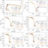 |
Fig. 1 Evolution of the models in the HR diagram for 10, 15, 20, 30, 60 and 100 M⊙. Evolutionary tracks for different initial rotational velocities at a given initial mass are given in each panel as indicated by the labels. The end points of core hydrogen burning and core helium burning are marked by an square and a cross, respectively, on each evolutionary track. |
The enhancement of the mass loss rate when the star approaches the ωΓ limit is reflected in the term (1/(1 − Ω))0.43. We evaluate Γ using the radiative opacity for the outermost layers where the optical depth is lower than 100. Because a singularity can occur at Ω = 1 according to Eq. (1), we limit the mass loss rate such that the mass loss time scale is longer than the thermal time scale of the star as in Yoon et al. (2010): ![Mathematical equation: \begin{equation} \label{eq3} \dot{M} = \mathrm{min}\left[ \dot{M}(v),0.3\frac{M}{\tau_\mathrm{KH}} \right], \end{equation}](/articles/aa/full_html/2012/06/aa17769-11/aa17769-11-eq241.png) (3)where τKH is the Kelvin-Helmoltz time scale, and Ṁ(v) is given by Eq. (1).
(3)where τKH is the Kelvin-Helmoltz time scale, and Ṁ(v) is given by Eq. (1).
The wind material that is mechanically ejected at the ωΓ limit may form a decretion disk. Recently, Krtička et al. (2011) argued that viscous coupling between the star and the decretion disk may significantly reduce the mass loss rate. This might potentially alter the final masses of the rotating models, but its detailed investigation is beyond the scope of the present study.
2.3. Initial conditions and model grid
The initial conditions and some important properties of the evolutionary models are summarized in Tables 1 and 2. We consider twelve different initial masses (Minit = 10, 15, 20, 30, 60, 100, 150, 200, 250, 300, 500, and 1000 M⊙). Several different initial rotational velocities were considered at each mass, from zero to 80% of the Keplerian value (vK) at the equatorial surface. Solid-body rotation was assumed for the initial velocity profile. The initial mass and the initial rotational velocity are denoted by the model sequence number. For example, the sequence “m100vk04” indicates Minit = 100 M⊙ and vinit/vK = 0.4.
In metal-free massive stars, the CNO cycle cannot be activated initially. Because the energy generation due to the pp chain is too weak to support a massive star with M ≥ 20 M⊙ for a significant fraction of the evolutionary time, the stellar core rapidly contracts until enough carbon (i.e., X(C) ~ 10-10) is produced by helium burning at Tc ~ 108 K. Hydrogen burning with the CNO cycle only begins thereafter. This makes it difficult to make a relaxed model on the zero-age main sequence for Pop III stars. For this reason, we included a small amount of 3He for the initial chemical composition, which may result from deuterium burning, such that X(H) = 0.76, X(4He) = 0.23999 and X(3He) = 0.00001. In this way, all our initially relaxed models are supported by the energy generation due to 3He burning, and the radii of our initial models are much larger than those obtained when the main sequence begins. Although this initial configuration looks artificial, it is not unrealistic given that the first stars should undergo rapid mass accretion phase that leads to significant expansion of the envelope before they reach the zero-age main sequence (ZAMS) (Omukai & Palla 2003; Ohkubo et al. 2009).
In Table 1, we provide the information for the mass and rotational velocity when the stars arrive on the ZAMS, as well as their initial values. Given the efficient transport of angular momentum by the Spruit-Tayler dynamo, near solid-body rotation is maintained during this initial contraction phase. It should be noted that Ekström et al. (2008) determined rotational velocities only when the stars are close to the ZAMS, and thus our ZAMS values should be compared with theirs, and not with our initial values.
3. Basic results
3.1. Evolution on the Hertzsprung-Russell diagram
Figures 1 and 2 show the evolutionary tracks of all of our models in the Hertzsprung-Russell (HR) diagram. As mentioned above, our initially relaxed models are supported by 3He burning. Once the evolution starts, 3He is very quickly destroyed and the stars undergo rapid contraction until they reach the ZAMS. The time scale of this initial contraction phase ranges from 104 to 3 × 10⁵ yr, depending on the initial mass. The models with Minit = 10 and 15 M⊙ are powered by pp-chains for a significant fraction of the main sequence lifetime (13.3 Myr and 2 Myr, respectively, for non-rotating models). Thereafter, the CNO cycle becomes dominant, which is marked by the smooth turn-over toward lower temperature in the HR diagram. For Minit ≥ 20 M⊙, the stars are already supported by the CNO cycle on the ZAMS, which agrees well with the previous work (Marigo et al. 2001; Ekström et al. 2008).
Compared to the models in the previous work, our non-rotating models become redder in the HR diagram during the post-main sequence phases. As an example, the surface temperature of the non-rotating 15 M⊙ models becomes log Teff = 4.3 and 4.5 in Marigo et al. and Ekström et al., respectively, while it becomes as low as log Teff = 3.9 in our case. In addition, our non-rotating models with M ≥ 150 M⊙ become red-supergiant stars already during core hydrogen burning, while M > 250 M⊙ was needed in Marigo et al. for this to happen. This must result mainly from the fact that our adopted overshooting parameter is larger: ~ 0.3 HP and 0.2 HP are used in Marigo et al. and Ekström et al., respectively, while 0.335 HP in the present study. The larger overshooting parameter also has an impact on the size of the stellar core and the evolutionary time. For example, the main sequence lifetime (τH) and the helium core size (MHe − Core) of our non-rotating 200 M⊙ model are 2.40 Myr and 114 M⊙, respectively, (see Table 2), compared to 2.27 Myr and 102 M⊙ in Ekström et al.
Rotating models start at lower surface temperature and luminosity in the HR diagram for larger vinit/vK, reflecting the effect of the centrifugal force on the stellar structure. Rotationally induced mixing, on the other hand, tends to increase the size of the convective core and the surface helium abundance. The latter effect becomes dominant as the star evolves, leading to higher luminosity and higher surface temperature than those in the corresponding non-rotating models, for most of the time on the main sequence. The evolutionary time also becomes systematically longer for higher initial rotational velocity because of the larger convective core. The central temperature is initially lower for higher initial rotational velocity because of the effect of the centrifugal force, but becomes higher already in the early phase of core hydrogen burning than those in a corresponding lower velocity model, as the convective core becomes larger in the rotating models due to rotationally induced chemical mixing. For instance, the center of the 100 M⊙ star enters the pair instability regime for vinit/vK = 0.6, while it does not in the corresponding non-rotating sequence (see Fig. 3). The final fate of such a massive star can be significantly influenced in this way, as discussed in Sect. 6.
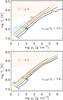 |
Fig. 3 Evolution of the central temperature and density in some model sequences for vinit/vK = 0 (upper panel) and vinit/vK = 0.6 (lower panel). The initial masses are marked by the labels in the figures. The regime for the pair-instability is marked by pink shading. |
One of the most dramatic effects of rotationally induced chemical mixing may be the so-called chemically homogeneous evolution (CHE; Maeder 1989), which can be observed with the blueward evolutionary tracks in Figs. 1 and 2. We find that CHE can occur for a certain range of the initial mass (15 ≤ Minit ≤ 200 M⊙) if the initial rotational velocity is sufficiently high. For some cases, the star follows the CHE track for most of the main sequence phase but afterwards moves rapidly to the right in the HR diagram, in particular during the post-main sequence phases. Such transitionary evolution is found in Seqs. m200vk04, m250vk04 and m250vk06, for example. In the present study, we define these three different evolutionary patterns, i.e., normal evolution (NE), CHE, and transitionary evolution (TE), according to the following criteria.
-
NE: The mass fraction of helium at the surface (Ys) remains smaller than 0.7 until the end of the main sequence. The star generally moves redwards in the HR diagram throughout the evolution.
-
CHE: Ys becomes larger than 0.8 by the end of the main sequence. The star generally moves bluewards throughout the evolution.
-
TE: Ys becomes larger than 0.7 by the end of the main sequence. The star follows the CHE track until the end of the main sequence, but moves redwards during the post-main sequence phases.
3.2. Internal structure
Figure A.1 shows the internal structure for model sequences with vinit/vK = 0.0, 0.2, 0.4 and 0.61. Note that the relative size of the convective core compared to the total mass becomes larger for higher initial mass, which is the well-known effect of higher radiation pressure in more massive stars. We find that the convection zone in the envelope extends up to the near-surface layers during the post-main sequence phases in all of our non-rotating models except for Minit = 15 and 20 M⊙. This outer convective zone is not developed for M ≤ 60 M⊙ in Ekström et al. (2008) for their non-rotating case. This difference must originate from the larger overshooting parameter adopted in the present study than in Ekström et al., as explained above. The convective carbon-burning core is not developed for M ≥ 20 M⊙ in our models, which agrees well with the previous studies (Chieffi & Limongi 2004; Ekström et al. 2008; Heger et al. 2000).
Interestingly, in non-rotating models of M ≥ 200 M⊙, the inner boundary of the convective envelope begins to penetrate into the layers that have previously undergone hydrogen shell burning during core helium-burning phase. This eventually leads to a dredge-up of helium core material, and hot bottom burning occurs afterwards where primary nitrogen is abundantly produced. We discuss this phenomenon below in greater detail (Sect. 4).
Rotating models have a larger helium core and a smaller convective envelope than those in the corresponding non-rotating models, which is an effect of rotationally induced chemical mixing. Dredge-up of helium core material by the downward penetration of the convective hydrogen envelope does not occur any more with rotation. The envelope remains radiative in the CHE models.
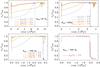 |
Fig. 4 Rotational velocity in units of the critical velocity (vcrit) given by Eq. (2) as a function of time for model sequences with Minit = 30, 100, 200, and 500 M⊙. The initial rotational velocity in units of the Keplerian value (vK) is indicated by the labels. Note that |

3.3. Rotation and angular momentum
Figure 4 shows the evolution of the surface rotational velocity in the rotating model sequences for 30, 100, 250 and 500 M⊙. It rapidly increases during the initial contraction phase, and decreases for a short period when the star begins to expand on the ZAMS. Note that in model sequences with vinit/vK ≥ 0.4, the critical rotation is achieved during this initial contraction phase, leading to mass shedding even before the star arrives on the ZAMS. This is the reason why, in Table 1, the masses on the ZAMS for these rapidly rotating models are somewhat smaller than the initial masses.
Soon after the ZAMS, the surface rotational velocity gradually increases again, which is an effect of the internal transport of angular momentum. On the main sequence, the density of the hydrogen-burning core increases as the mean molecular weight increases as a result of nuclear burning. Although this tends to create differential rotation between the core and the envelope, magnetic torques due to the Spruit-Tayler dynamo keep the star rotating almost rigidly by transporting angular momentum from the core to the envelope. The outer layers are spun up accordingly, and most of our rotating models eventually reach the critical rotation on the main sequence. The critical rotation at the surface is achieved earlier and maintained for a larger fraction of the evolutionary time, for a higher initial rotational velocity. If the star becomes a red supergiant afterwards, the expansion of the envelope leads to a rapid decrease of the surface rotational velocity (v/vcrit < 0.1). With CHE, on the other hand, it still remains close to the critical limit (v/vcrit > 0.8) during the post-main sequence phases.
As prescribed in Eqs. (1)–(3), our models lose mass when the surface velocity approaches the critical limit. As shown in Tables 1 and 2, more mass is lost for higher initial rotational velocity. In the case of Minit = 250 M⊙, for example, the total mass ejected (ΔMej) is only about 1.0 M⊙ for vinit/vK = 0.2 (Seq. m250vk02), while it increases to about 60 M⊙ for vinit/vK = 0.6 (Seq. m250vk06). Our rotating models generally lose more mass than those of Ekström et al. (2008) for a given initial rotational velocity. For instance, our 60 M⊙ star in Seq. m60vk02 has a lower surface rotational velocity of 631 km s-1 on the ZAMS (see Table 1) than that of in Ekström et al. (800 km s-1), but the total amount of the ejected mass is significantly larger (ΔMej = 3.58 M⊙) than that of Ekström et al. (ΔMej = 2.32 M⊙). This is because our models reach the critical rotation earlier due to the Spruit-Tayler dynamo than those of Ekström et al., who did not include the effect of magnetic fields. Marigo et al. (2003), who assumed rigid body rotation in their models, adopted a low initial rotational velocity: 500 km s-1, which roughly corresponds to vZAMS/vK ≤ ~ 0.1 according to Figs. 6 and 7 in their paper. Their models therefore reach the critical rotation only briefly near the end of the main sequence, losing much less mass than our rotating models for a given initial mass. For example, the 250 M⊙ model in Marigo et al. gives ΔMej = 3.35 M⊙, while we have ΔMej = 16.4 M⊙ in Seq. m250vk02, for which vZAMS/vK = 0.36 (Table 1).
It is believed that the final fate of a massive star can be critically influenced by rotation of the core (e.g. Heger et al. 2000). For example, the so-called collapsar (Woosley 1993) is predicted to occur if the final angular momentum in the core is higher than the critical limit for the formation of an accretion disk around a rotating black hole at a given mass (jKerr,lso; see also the figure caption of Fig. 5; Bardeen et al. 1972). Figure 5 shows the evolution of specific angular momentum profile (jr) in four different model sequences (m30vk02, m30vk05, m200vk06, m500vk04). In Seq. m30vk02, where the star generally expands throughout the evolution, the core experiences strong braking due to the core-envelope coupling via the magnetic torque. The final angular momentum in the core becomes well below jKerr,lso. In Seq. m30vk06, on the other hands, the star of the same initial mass undergoes CHE, to become a massive helium star by the end of the main sequence and to avoid the core-envelope couping. The specific angular momentum in the core remains higher than jKerr,lso until the end of calculation (core neon exhaustion), meaning that this model meets all the requirements for long GRB progenitors within the collapsar scenario (Woosley 1993): high angular momentum in the core, large core mass to form a black hole, and absence of an extended hydrogen envelope. This implies that the CHE channel for the formation of long GRB progenitors can still be important for the first stars (see Yoon & Langer 2005; Yoon et al. 2006; Woosley & Heger 2006, for a more detailed discussion on GRB progenitors via CHE). Note that the condition for magnetar formation (j ≳ 4 × 1015 cm2 s-1; e.g.,Wheeler et al. 2000) is also satisfied in this model.
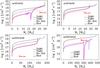 |
Fig. 5 Mean specific angular momentum over the shells as a function of the mass coordinate at different evolutionary epochs (ZAMS, TAMS, core helium exhaustion, and the last calculated model) in Seqs. m30vk02, m30vk06, m200vk06 and m500vk04, as indicated by the labels. The thin sold line labeled jKerr,lso denotes the specific angular momentum for the last stable orbit at the given mass of a black hole, assuming that all mass below forms a rotating black hole. Here, if the contained angular momentum is higher than that of a maximally rotating black hole, the black hole is assumed to rotate maximally. |
However, CHE does not always lead to retention of a large amount of angular momentum in the core such that j > jKerr,lso. In Seq. m200vk06, the specific angular momentum in the core decreases significantly below jKerr,lso before core helium exhaustion. Given the final mass of 146.43 M⊙, the star of this model sequence is supposed to explode as a pair instability supernova, but even if collapse into a black hole occurred, a GRB would not be produced in this case. We find that the CHE models have lower specific angular momentum in the core for larger initial mass, in general. This can be understood by the fact that the stellar structure of a rigidly rotating chemically homogeneous star is such that jr is smaller at a given mass coordinate, for a given v/vK as shown in Fig. 6. In the CHE models, the surface rotational velocity remains close to the critical rotation for most of the lifetimes (Fig. 4), while near-rigid rotation is maintained until core helium exhaustion. Significant differential rotation is developed only thereafter. In addition, higher mass stars have lower v/vK at the critical rotation because of the increased role of radiation pressure. The general tendency for smaller jr with larger mass in the CHE models results from these factors.
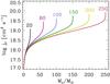 |
Fig. 6 Specific angular momentum as a function of the mass coordinate in the initial models with vinit/vK = 0.6 for different initial masses (20, 60, 100, 150, 200 and 250 M⊙) as indicated by the labels. |
For Minit ≥ 250 M⊙, CHE is not realized anymore, and expansion of the envelope to the red supergiant phase leads to strong core-braking as shown Fig. 5. As a result, the so-called super-collapsar (collapsar in stars of M > 250 M⊙) is not likely to occur. We discuss below the implications of our results for the final fate of the first stars in greater detail (Sect. 6).
3.4. Ionizing flux
Detailed information on the hydrogen and helium-ionizing flux emitted from our models is provided in Table 3. Black-body radiation is assumed for the calculation of energy and number of ionizing photons. Compared to Heger & Woosley (2010), our non-rotating models at a given mass produce more ionizing photons, which results from the larger overshooting parameter adopted in our study. Rotation tends to make stars brighter, bluer and live longer, and thus more ionizing photons are emitted than in the corresponding non-rotating case, in general. In Fig. 7, the total number of ionizing photons from the non-rotating models is compared to that from the rotating models with vinit/vK = 0.4, for hydrogen (H), neutral helium (He) and singly ionized helium (He+). The most notable change with rotation is found for ionization of He+. Here, the models with 20–150 M⊙ follow CHE, and the number of He+ ionizing photons increases by factors of 4–20. For H and He, enhancement of the number of ionizing photons is less prominent, but it is still significant for the CHE models, showing factor of 2–4 increase.
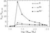 |
Fig. 7 Ratio of the total number of ionizing photons from non-rotating models to that from rotating models with vinit/vK = 0.4. The connecting lines of filled circles, triangles and squares give the values for hydrogen and first and second helium ionization, respectively. |
4. Effects of chemical mixing on the nucleosynthesis
The heavy elements synthesised in Pop III stars can be ejected into the surrounding medium by stellar winds and/or supernova explosions, which is supposed to critically influence the chemical evolution of the early Universe. Tables 4 and 5 present the yields for eight different isotopes in the wind material that has been ejected from the star throughout the evolution and in the last computed model, respectively, in each model sequence. Our non-rotating models do not experience mass loss at all, and therefore the wind yields of non-rotating models are not given in Table 4. The model sequences with Minit = 1000 M⊙ are not included in the tables either, because the calculations were terminated before the end of main sequence. The end points of the other models are mostly carbon burning or carbon exhaustion (see Table 2), and none of our models have undergone the late evolutionary phases beyond oxygen burning. Therefore, in Table 5, neither compact remnant mass nor explosive nucleosynthesis is considered. This means that the amounts of  ,
,  and
and  in Table 5 should be taken as an upper limit for the supernova yields since they would decrease during the latest evolutionary stages and the supernova explosion that are not followed in this study, while the yields for the other isotopes that are mostly located in the outer layers of the star would not change much from the end points of our calculation.
In Table 5, we also give the neutron excess at the center of the star (ηc) in the last model. Here, the neutron excess is defined as 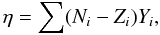 (4)where Ni, Zi and Yi denote neutron number, proton number, and abundance of isotope i, respectively. The last column of the table gives the maximum mass fraction of 14N (Xmax(14N)) that has been achieved during the evolution.
In the following subsections, we discuss how convection and rotationally induced chemical mixing influence the nucleosynthesis in our models.
4.1. Convective mixing
During the post-main sequence phases, convection can induce mixing of helium-burning products (notably 12C and 16O) into hydrogen-shell-burning layers, boosting the CNO cycle. We find that there exist two different ways for this mixing. The first one is penetration of the helium convection zone (either convective helium core or convective helium-burning shell) into the hydrogen-burning shell, which has also been found by Ekström et al. (2008) and Heger & Woosley (2010). The second way is penetration of the convective hydrogen envelope into the helium core, which occurs for Minit ≥ 200 M⊙ in our models. To our knowledge, the latter has not been reported in the previous work.
Penetration of the convective helium burning shell into the hydrogen-burning shell occurs for Seqs. m20vk02, m30vk00, m100vk00 and m150vk02. In the Kippenhahn diagram of Seq. m20vk02 (Fig. A.1), for instance, the convection zone of the helium-burning shell continuously extends upwards and reaches the bottom of the hydrogen-burning shell when tf − t ≃ 10 yr. The consequent mixing of carbon into the hydrogen-burning shell induces boosting of the CNO cycle, and the hydrogen shell becomes convective. This produces a large amount of primary nitrogen.Xmax(14N) in Seq. m20vk02 becomes as large as 10-3 (see Table 5), which is 1000 times larger than in the case without this mixing (i.e.,Xmax(14N) ≃ 10-6 in Seqs. m20vk00 and m20vk03). In terms of the total yield of nitrogen ( ) it is about 10000 times higher than in Seqs. m20vk00 and m20vk03. However, remains smaller than those in the corresponding CHE models that experience strong rotationally induced chemical mixing: e.g., M14N ≃ 10-3 M⊙ in Seq. m20vk02, while M14N ≃ 10-2 M⊙ including the wind yield (Tables 4 and 5).
In these sequences, a small amount of hydrogen is also mixed into the convective region of the helium-burning shell. Given the large mass fraction of carbon and the fairly high temperature (~2 × 10⁸ K) in this region, the nuclear time scale for hydrogen burning becomes shorter than the convective turn-over time scale. This rapid nuclear burning in convective layers cannot be properly described with our code because the nuclear network and the transport equation are calculated in succession. This leads to an overestimate of the energy generation rate here since the hydrogen mass fraction at the bottom of the convection zone above the helium burning shell can become artificially higher than it should be. However, we find that the overall amount of nitrogen and energy produced in this region is small compared to that of the hydrogen-burning shell. In addition, our calculations are terminated soon after this mixing occurs, and this uncertainty should not affect the main conclusions of the present study.
Penetration of the convective helium-core into the hydrogen-burning shell can be most prominently observed in Seqs. m100vk00 and m150vk02. Here, the convective helium core grows and reaches the bottom of the hydrogen-burning shell, as shown in Fig. A.1. In this case, a significant fraction of the newly produced primary nitrogen in the hydrogen shell source is mixed into the convective helium core, enhancing the neutron excess in the core, which is discussed below in Sect. 4.3.
On the other hand, our non-rotating models with Minit ≥ 200 M⊙ experience dredge-up of the helium core material into the hydrogen-burning shell by convection in the hydrogen envelope (see Fig. A.1). As an example, the detailed structure around the boundary between the helium core and the hydrogen envelope is shown in Fig. 8, for Seq. m500vk00. The hydrogen envelope becomes convective already on the main sequence and the convection zone progressively extends downwards. During core helium burning, it eventually penetrates the layers that previously belonged to the convective helium core. A large amount of carbon and oxygen, which has been produced by core helium burning, is thus mixed into the hydrogen envelope, boosting the CNO cycle at the bottom of the convection zone. Figure 9 shows that the mass fraction of the CNO elements in the 500 star model becomes as large as 0.03, after this dredge-up history.
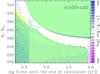 |
Fig. 8 Kippenhahn diagram for Seq. m500vk00, which is same as in Fig. A.1 but zoomed up for 200 ≤ Mr/M⊙ ≤ 350, and 4.0 ≤ log (tf − t) ≤ 5.7. Here tf is the evolutionary time at the end of calculation. |
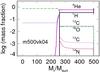 |
Fig. 9 Mass fraction of different isotopes in the last model of Seq. m500vk00. |
We find that this convective dredge-up of the helium core material becomes more efficient for more massive stars, in general. The total yields of 13C and 14N increase from 1.5 × 10⁻³ M⊙ and 3.71 × 10⁻⁴ M⊙ in 200 M⊙ model to 0. 0.34 M⊙ and 0.12 M⊙ in 500 M⊙ model, respectively. Note that in our non-rotating models, the outermost layers of about 0.1 M⊙ remain radiative even when the most part of the hydrogen envelope becomes convective. Since chemical mixing cannot occur beyond the convection zone without rotation, the initial values are maintained for the chemical composition at the surface. This is the reason for the sudden change in the mass fractions of the isotopes near the surface in Fig. 9. No mass loss occurs in our non-rotating model sequences, given our wind prescription that allows stellar winds only with surface-enrichment of heavy elements (Sect. 2.2). In reality, massive stars may become unstable to the pulsational instability, which may cause mass loss (Baraffe et al. 2005). Pulsation caused by partial ionization of hydrogen may be particularly important during the red supergiant phase, when the above-discussed convective dredge-up can occur efficiently. Therefore, we cannot exclude the possibility of significant mass loss from non-rotating massive Pop III stars, and the consequent enrichment of the CNO elements into the circumstellar material. Because pulsation-driven winds from RSG stars must be slow, it should have interesting consequences in the chemical evolution history as in the case for massive AGB stars (e.g., Ventura et al. 2001). Even formation of dusts around such Pop III RSG stars might be possible, given the high abundance of CNO elements in the envelope (Fig. 9). This question deserves more studies.
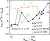 |
Fig. 10 Total yields of nitrogen as a function of the initial mass for vinit/vK = 0.0 (star symbol), 0.2 (open circle) and 0.4 (filled circle). For vinit/vK = 0.4, the CHE models are marked with a yellow color, while the NE/TE models with a purple color. The connecting line with open triangles gives the nitrogen yields of the rotating models by Ekström et al. (2008). |
4.2. Rotationally induced mixing
The significance of rotationally induced chemical mixing on nucleosynthesis varies according to the initial rotational velocity for a given initial mass. As shown in Fig. 10 (see also Tables 4 and 5), in most of the slowly rotating models that follow NE, the total yield of primary nitrogen is not higher by more than a factor of 10 than in the corresponding non-rotating case, if the star does not experience the encroachment of the helium convection zone into the hydrogen shell source. For instance, Seq. m100vk00 gives M14N = 2.87 × 10⁻⁶ M⊙, while Seq. m100vk02 gives M14N = 3.29 × 10⁻⁶ M⊙. For models with Minit = 30, 200, 300 and 500 M⊙, is even larger in non-rotating sequences than in the corresponding sequences with vinit/vK = 0.2. This is because these non-rotating massive stars undergo the convective mixing discussed above: penetration of the convection zone of the helium-burning shell into the hydrogen-burning shell for Minit = 30 M⊙, and the convective dredge-up of the helium core material for Minit = 200, 300 and 500 M⊙. On the other hand, Seqs. m20vk02 and m60vk02 give exceptionally large (8.14 × 10⁻⁴ and 9.21 × 10⁻⁵ M⊙, respectively), compared to the other cases with the same initial velocity. This is not because of the rotational mixing, but because of the convective mixing between the convective helium shell and the hydrogen shell source.
The CHE models produce more primary nitrogen by several orders of magnitude than in the corresponding non-rotating or slowly rotating case, in most cases. For instance, Seq. m30vk04 gives M14N = 0.024 M⊙, compared to 1.19 × 10⁻⁷ M⊙ in Seq. m30vk00. Although they evolve almost chemically homogeneously throughout the main sequence, some amount of hydrogen is still left in the outermost layers, which undergoes hydrogen shell burning during the core helium-burning phase (see Figs. A.1 and 11). Chemical mixing induced by rotation between the helium core and the hydrogen shell then leads to abundant production of primary 14N and 13C, as well as 22Ne (see Fig. 11 for such an example).
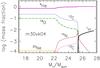 |
Fig. 11 Mass fraction of different isotopes in Seq. m30vk04, when primary nitrogen is abundantly produced during core helium burning. |
The total yields of primary nitrogen in the rotating models by Ekström et al. (2008) are compared with ours in Fig. 10. In their study, where magnetic torques are not considered for the transport of angular momentum, none of the models follows CHE, and the production of primary nitrogen is enhanced mainly by chemical mixing due to the shear instability during the core helium-burning phase, where a strong degree of differential rotation is developed across the boundary between the helium core and the hydrogen envelope. In our models with the Spruit-Tayler dynamo, the role of the shear instability is negligible because near rigid-body rotation is maintained until the end of core helium burning. In our NE models, chemical mixing by the Eddington-Sweet (ES) circulations becomes rather inefficient during the post-main sequence phase, because the strong chemical stratification between the helium-burning core and the hydrogen envelope significantly slows down the ES circulations. This explains the weak production of primary nitrogen in our rotating NE models compared with the rotating models by Ekström et al. In the CHE models, however, the inhibition of the ES circulations by the chemical stratification is much less significant and the total yields of primary nitrogen are comparable to those of Ekström et al. The yields of other isotopes like 13C, 18O and 22Ne also increase by several orders of magnitude with CHE.
As shown in the Kippenhahn diagrams in Fig. A.1, the CHE models with Minit ≤ 150 M⊙ lose the hydrogen-burning shell layers before the end of the core helium-burning phase. Note that the mass loss here is dominated by the mechanical winds, which must be slow. Slow ejecta of hydrogen-burning products via either winds from massive AGB stars or mechanical winds from massive single or binary stars are often invoked to explain some chemical anomalies observed in globular clusters, characterized by enrichment of He, N, Na and Al, and depletion of C and O (Ventura et al. 2001; Denissenkov & Herwig 2003; Prantzos & Charbonnel 2006; Decressin et al. 2007; de Mink et al. 2009). As shown in Table 4, the wind materials of our CHE models are indeed marked by enrichment of He and N, but the amounts of C and O may be too large to explain the anomalies. We will address the implications of these models for the chemical evolution in the early Universe in a future paper.
4.3. Neutron excess
The neutron excess (Eq. (4)) in the stellar core is one of the most important factors that determine the nucleosynthesis of a supernova explosion. This is particularly the case for the pair-instability supernova (PISN). Detailed calculations by Heger & Woosley (2002) showed remarkable deficiency of odd-charge elements in the yields of PISNe from Pop III stars, which results from very low neutron excess. Despite the theoretical expectation of frequent PISN explosions in the early Universe, such a peculiar abundance pattern has not been found in the observed very metal-poor stars, which are believed to conserve the signatures of the nucleosynthesis in the first generations of stars. It should be noted, however, that Heger & Woosley (2002) only calculated pure helium star models, ignoring the complicated history of chemical mixing that is discussed above. It is therefore important to investigate whether or not the convective and/or rotational mixing can significantly increase the neutron excess in Pop III PISN progenitors.
In Table 5, we show the value of the central neutron excess (ηc) at the end of calculation for each evolutionary sequence. In our calculations, the major source for the neutron excess is the 14N(α,γ)18F(e + ,ν)18O reaction, which can occur in helium-burning layers. This means that ηc in our models is determined by the amount of primary nitrogen mixed into the helium-burning core, and does not include any excess beyond helium burning. On the other hand, Heger & Woosley (2002) include many more reactions that can further increase the neutron excess during the advanced stages beyond helium burning (e.g., the 20Ne(p,γ)21Na(e + ,ν)21Ne reaction during carbon burning and many other weak processes). The implication is that the problem with the deficiency of odd-charged elements would not be solved by chemical mixing of primary nitrogen, unless the values of ηc in our models were significantly higher than those of Heger & Woosley.
As discussed below (Sect. 6), PISNe are expected for 120 ≲ Minit/M⊙ ≲ 240 with NE, and 84 ≲ Minit/M⊙ ≲ 200 with CHE. For this mass range, the neutron excess in our models is limited to ~10-5, which is much lower than those of the Pop III star models by Heger & Woosley (2002) (ηc ~ 10-4). Therefore, we conclude that PISNe from our models would not result in a significantly different nucleosynthesis compared to that of Woosley & Heger’s models. It should be investigated in future if this conclusion would still hold with non-magnetic models, where strong mixing due to the shear instability would occur during the post-main sequence phases (Ekström et al. 2008).
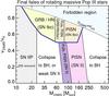 |
Fig. 12 Phase diagram for the final fates of massive Pop III stars, in the plane of the mass and the fraction of the Keplerian value of the equatorial rotational velocity on the zero-age main sequence. The dotted line denotes the limit above which the rotational velocity at the surface would exceed the critical rotation velocity (vcrit in Eq. (2)). The thick solid line marks the boundary between the regimes for the chemically homogeneous evolution (CHE), and the non-CHE evolution (normal evolution or transitionary evolution; see Sect. 3). The regions for different final fates are divided by thin solid lines. Each acronym has the following meaning. SN IIP: Type IIP supernova, NS: neutron star, BH: black hole, SN II: type II supernova, PISN: pair-instability supernova, Puls. PISN: pulsational pair-instability supernova, GRB: gamma-ray bursts, HN: hypernova, SNIbc: type Ib or Ic supernova. |
5. Conditions for chemically homogeneous evolution
The CHE has important consequences not only for the nucleosynsthesis, but also for the final fate of massive Pop III stars (Sect. 6). We give the boundary for CHE in Fig. 12 in the plane spanned by the initial mass and the surface rotational velocity2 (see Sect. 6 for more detailed explanation on the figure). Our results indicate that CHE would not occur for MZAMS ≲ 13 M⊙ and MZAMS ≳ 190 M⊙. The limiting rotational velocity for CHE continuously decreases from MZAMS = 13 M⊙ to about 60 M⊙, and rapidly increases from about 150 M⊙ until it reaches the forbidden region at MZAMS ≃ 190 M⊙. The mass dependency of the limiting vZAMS for CHE can be understood as follows.
In our models, chemical mixing is dominated by Eddington-Sweet (ES) circulations. According to Kippenhahn (1974), who we follow for the prescription of ES circulations in our models, the circulation velocity in a radiative region is given as
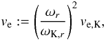 where
where 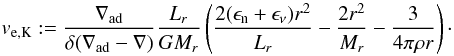 (5)Here ωr is the angular velocity at a radius r, ωK,r the local Keplerian value, ϵn the nuclear energy generation rate, ϵν the energy loss rate due to neutrino emission, and Lr the local luminosity. The other symbols have their usual meaning. Note that ve becomes ve,K when ωr = ωK,r.
The chemical stratification tends to slow down the circulation velocity, and a correction is made for the actual circulation velocity in our models (Heger et al. 2000):  (6)where
 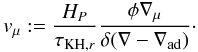 (7)Here τKH,r is the local Kelvin-Helmoltz time-scale at a radius r.
For the discussion below, we define three different time scales: 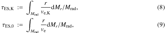 and
and 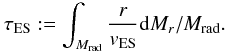 (10)Here Mrad denotes the total mass of the radiative layers in the envelope. Note that τES,K does not depend on the rotational velocity, and thus can be used as a “susceptibility” of a fluid to ES circulations, for a given thermodynamic condition. On the other hand, τES,0 represents the ES circulation time scale for chemically homogeneous layers since the effect of a chemical stratification is not included in ve. Given that
 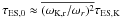 (see Eq. (5)), the ratio τES,0/τES,K gives information on how the ES circulation is influenced by rotation in stars. For example, loss of angular momentum and/or expansion of a star would result in an increase of τES,0/τES,K. Finally, τES is the real ES circulation time that considers the stabilizing effect of a chemical stratification. The ratio τES/τES,0 can be used as a measure of chemical inhomogeneity inside a star: τES/τES,0 = 1 for ∇μ = 0 and τES/τES,0 > 1 otherwise.
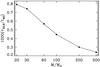 |
Fig. 13 τES,K in Eq. (8), divided by the main sequence lifetime (tMS) and multiplied by 1000, as a function of the initial mass. The ZAMS models of 20, 30, 60, 100, 250 and 500 M⊙ were used for the evaluation of τES,K. |
It should be noted that the actual time scale of ES circulations in stellar evolution models is much larger than the above defined τES, as a result of the calibration of the mixing efficiency with observational data (see Sect. 2). Therefore, our discussion below should be considered as only indicative.
We present the ratio of τES,K to the main sequence lifetime (tMS) as a function of initial mass in Fig. 13, to investigate how thermodynamic conditions vary according to the initial mass in favor/disfavor of ES circulations. Here, τES,K is estimated on the ZAMS for each mass. The figure shows that τES,K/tMS is systematically smaller for a higher mass star. This is related to higher radiation pressure and lower density in a higher mass star. This means that, for a given initial rotation velocity, CHE should be favored in a higher mass star. This may explain why the limiting rotation velocity for CHE continuously decreases with increasing mass from 13 M⊙ to about 60 M⊙ in Fig. 12.
However, the influence of mass loss becomes important for very massive stars: as discussed in Sect. 3.3, more massive stars can reach the critical rotation in an earlier evolutionary phase, losing more mass and angular momentum. This effect is reflected in the evolution of τES,0/τES,K that is shown in the upper panel of Fig. 14 for some model sequences with vinit/vK = 0.4. τES,0/τES,K increases very rapidly in 250 M⊙ and 500 M⊙ stars, compared to those in lower mass stars. For example, in 500 M⊙ star, τES,0/τES,K increases by a factor of two from its initial value, when the central helium mass fraction (Yc) becomes about 0.4. Since the change of the radius during this period is only moderate (from 12 R⊙ to 15 R⊙), the rapid increase in τES,0/τES,K results mainly from the loss of angular momentum due to centrifugally-driven mass loss.
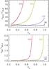 |
Fig. 14 Upper panel: the evolution of τES,0/τES,K (see Eqs. (8) and (9)) in the model sequences m30vk03, m100vk04, m250vk04 and m500vk04. Only main sequence models are considered here. Bottom panel: the evolution of τES/τES,0 (see Eqs. (9) and (10)) in the corresponding model sequences. |
The evolution of τES/τES,0 is shown in the bottom panel of Fig. 14. For 30 M⊙ and 100 M⊙ models, τES/τES,0 ≃ 1.0 is maintained until the end of main sequence, as a result of CHE. For 250 M⊙ and 500 M⊙, τES/τES,0 starts deviating from 1.0 at Yc ≃ 0.6 and Yc ≃ 0.4, respectively. This indicates that although these stars initially follow CHE, chemical mixing due to the ES circulation becomes inefficient later as they progressively lose large amounts of angular momentum. This interpretation is confirmed by Fig. 15, which shows the evolution of surface helium mass fraction (Ys) as a function of central helium mass fraction (Yc), for model sequences of m30vk04, m250vk04 and m500vk04. Note that Ys is larger in 250 M⊙ and 500 M⊙ stars until Yc ≃ 0.6 and 0.4, respectively, than in 30 M⊙. This implies that chemical mixing is initially more efficient in those very massive stars than in 30 M⊙ star, although they eventually deviate from CHE because of angular momentum loss.
This means that without angular momentum loss, the CHE regime in Fig. 12 would extend to larger masses. Specifically, given that τES ∝ (vK/vZAMS)2τES,K, the result shown in Fig. 13 implies the limiting vZAMS/vK for CHE would decrease from 0.74 for 20 M⊙ to about 0.4 for 500 M⊙ in Fig. 12, if there were no loss of angular momentum.
From the above analysis, we draw the following conclusions.
-
Thermodynamic conditions are generally more favorable forchemical mixing by the ES circulation in more massive stars.Therefore, the limiting rotational velocity for CHE can decreasewith increasing mass, as long as the ES circulation is notsignificantly slowed down through angular momentum loss.
-
Critical rotation can be more easily achieved in more massive stars, since their surface luminosity is close to the Eddington limit. The consequent rapid loss of mass and angular momentum eventually tends to inhibit CHE in very massive stars (>~200 M⊙), even if rotationally induced chemical mixing is initially very efficient.
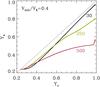 |
Fig. 15 Mass fraction of helium at the surface (Ys) as a function of the mass fraction of helium at the center (Yc) during the main sequence for model sequences m30vk04, m250vk04 and m500vk04. The thin dotted line corresponds to the case of perfect chemical homogeneity. |
6. Implications for the final fate
In Fig. 12, we present a phase diagram of the expected final fates of rotating massive Pop III stars in the plane of the mass and the rotational velocity in units of the Keplerian value. Note that here we used the ZAMS values instead of the initial values for mass and rotational velocity (see Table 1 and discussion in Sect. 2.3). To determine the boundaries for different regimes, we use interpolated values between the grid points of our calculated models, when it was needed.
The forbidden region in the figure is the regime where the surface rotational velocity exceeds the critical limit vcrit (Eq. (2)). Any star in this region would be unstable, experiencing mass eruption, and forced to come back to the regime of sub-critical rotation. The CHE regime (vCHE ≤ vZAMS ≤ vcrit) is marked by a thick solid line. Both NE and TE regimes are below this limit. Because our model grid is not fine enough to clearly identify the TE regime, we do not distinguish the two in the non-CHE regime in the figure. In any case, the parameter space for TE in this plane should be very small, located in the vicinity of the border of the CHE regime.
6.1. Core collapse supernovae
In the NE regime, the lower mass limit for black hole (BH) formation is simply assumed to be 25 M⊙. We did not follow the evolution up to iron core formation, and we cannot discuss how rotation would change the pre-supernova structure, which may affect this limit. However, in all models in the NE regime, the amounts of angular momentum in the core fall below the limit for magnetar (i.e., j ≳ 4 × 1015 cm2 s-1 in the innermost 1.4 M⊙; e.g., Wheeler et al. 2000) or collapsar formation (i.e., j ≳ 4 × 1016 cm2 s-1 in the layers that would be accreted to the black hole; Woosley 1993), by the end of core helium burning. This means that a jet-driven supernova or hypernova-like event powered by rotation may not occur in stars having hydrogen-rich envelopes, which have been discussed in Heger et al. (2003) in detail. Type IIP supernovae via usual core-collapse to a neutron star are expected for 8 M⊙ ≲ MZAMS ≲ 25 M⊙, and weak fall-back SNe or direct collapse to BH would occur for the other mass range outside the pair-instability regimes.
The light curve, luminosity, and chemical yields of a SN IIP are critically affected by the radius of the progenitor star at the pre-supernova stage. Our 10 M⊙ models expand to the red-supergiant phase, having the final radii of Rf ≃ 450 R⊙. 15 and 20 M⊙ models remain relatively blue up to core carbon exhaustion, having Rf ≃ 130...150 R⊙ and Rf ≃ 100 R⊙, respectively. We find these values do not change much with rotation in the NE regime, but they may still be affected by uncertain factors such as core overshooting and production of primary nitrogen, as discussed in Sects. 3 and 4.
6.2. Pair-instability supernovae
In the present study, we did not follow the explosive nuclear burning caused by pair instability and thus our models do not provide an exact boundary for the PISN regime. For the phase diagram of Fig. 12, we simply adopted the mass limits given by Heger & Woosley (2002): pulsational pair-instability SNe (puls-PISN) for helium core masses of 40 ≤ MHe,core/M⊙ ≤ 64, and pair-instability SNe (PISN) for 64 ≤ MHe,core/M⊙ ≤ 133. Note that these limits are based on non-rotating stellar models, and that the effect of the centrifugal force can lead to an upward-shift of each boundary with rotation (Glatzel et al. 1985). Because in our potential PISN progenitor models the rotational velocity in the innermost layers does not exceed a few percent of the local Keplerian values even in the case of CHE, the role of rotation may be minor. But more detailed studies should be carried out for clarifying the uncertainty3.
In the NE regime, the mass limits for puls-PISN and PISN decrease with rotational velocity, because the helium core mass increases with rotation. In the CHE regime, they do not change much with rotation, since in this case, the whole star is transformed to a helium star by complete mixing by the end of the main sequence. The progenitors of PISNe in the NE regime have a very extended hydrogen envelope with Rf ≃ 3000...5000 R⊙, depending on the mass. As shown in the recent calculations by Kasen et al. (2011), these PSNE would be marked by a long plateau phase of the light curve (100–400 days), and strong hydrogen lines (absorption and/or emission) in the spectra. In the CHE regime, the progenitors of puls-PISNe and PISNe do not have any hydrogen. The total amount helium at the pre-SN stage is small, ranging from 0.3 to 0.7 M⊙ (Table 5). A PISN from a CHE model is thus likely to appear as a SN 2007bi-like event, which is a very bright SN Ic (Gal-Yam et al. 2009), if the final mass of the progenitor is high enough ( ≳ 90 M⊙) to produce a large amount of nickel (Heger & Woosley 2002; Kasen et al. 2011).
6.3. Gamma-ray bursts
If specific angular momentum in the CO core is higher than jK,lso, and if the helium core mass is not within the range of PISNe, a collapsar may occur. In the NE regime, no collapsar formation is expected because angular momentum is too low in the core, while the conditions for a collapsar are fulfilled for stars of 13 ≲ MZAMS/M⊙ ≲ 84, in the CHE regime. The innermost cores (~1.4 M⊙) in the stars in the same regime also have high angular momentum to produce a magnetar (j ≳ 5.4 × 1015 cm s-1). Therefore, stars in this regime may be considered as GRB progenitors within both the collapsar scenario (Woosley 1993; Macfadyen & Woosley 1999) and the magnetar scenario (e.g., Duncan & Thompson 1992; Wheeler et al. 2000; Bucciantini et al. 2009)4.
Interestingly, both puls-PISN and GRB are expected for 56 ≲ MZAMS/M⊙ ≲ 84 in the CHE regime. In this case, pulsational pair-instability that occurs after carbon burning in the core may eject several solar masses, probably episodically (Woosley et al. 2007). The chemical composition of the puls-PISN ejecta would be characterized by large amounts of carbon and oxygen, and some helium (~0.3 M⊙). Only about several years thereafter, a GRB would be produced when the core collapses. Therefore, the GRB jet should interact with the very dense ejecta, which might result in an extremely luminous afterglow if the GRB jet were energetic enough. Heger et al. (2003) also suggested the possibility of occurrence of both puls-PISN and GRB from the same progenitor for very low metallicity. However, in their scenario, the puls-PISN is supposed to eject the hydrogen-rich envelope from the progenitor, while in our scenario based on the CHE models, no hydrogen would be contained in the ejecta of the puls-PISN. The accompanied supernova (if it were not out-shined by the GRB afterglow) would not appear as a SN 2006gy-like event (luminous type IIn Smith et al. 2007) but rather look like a Quimby-type supernova (Quimby et al. 2011) or a SN Ibn if helium were excited as a result of the interaction (Foley et al. 2007; Pastorello et al. 2007).
The GRB progenitors with 12 ≲ MZAMS/M⊙ ≲ 56 may not suffer the pulsational pair-instability. In these models, however, the critical rotation is maintained at the surface for a significant fraction of the evolutionary time, which leads to significant mass loss (Fig. 4). In particular, the mass loss rate becomes very high during the last 104 − 105 yrs, because of the rapid decrease of the radius of the star (Fig. 1). The mass loss would predominantly occur via a decretion disk in this case, and radiation driven winds along the poles must be very weak or negligible (see Sect. 2). This may lead to a very complex, highly aspherical structure of the circumstellar medium, which might be imprinted on the afterglow (see van Marle et al. 2008, for a related study).
Recently several authors investigated possible observational signatures from collapsars in very massive stars with M > 250 M⊙ (Komissarov & Barkov 2010; Mészáros & Rees 2010; Suwa & Ioka 2011; Toma et al. 2011). Our result implies that a GRB-like event from such a super-collapsar may not occur. First of all, CHE is inhibited for very massive stars (Sect. 5), and consequently they are expected to have a very extended hydrogen envelope, from which a jet from the central engine may not break out easily. Even if CHE were realized, the final angular momentum in such a massive star would not be high enough to produce a GRB (see discussion in Sect. 3.3). Suwa & Ioka (2011) argued that for very massive stars, accretion of the long-lived hydrogen envelope would result in jet-breakout even if they had a supergiant envelope. However, our 250, 300 and 500 M⊙ models show that the specific angular momentum would become well below jK,lso for the entire mass range including the hydrogen envelope, at the pre-collapse stage (Fig. 5). Direct collapse of the whole star into a BH without any remarkable visible event is the most likely outcome in this case. Although this conclusion is based on our assumption of the presence of weak-seed magnetic fields in Pop III stars, our preliminary results show that necessary conditions for a super-collapsar still cannot be easily fulfilled even without the assumption of magnetic fields (Yoon et al., in prep.).
According to theoretical studies on the formation of the first stars in the early Universe, Pop III stars may have two different classes in terms of initial mass function (Johnson & Bromm 2006; Yoshida et al. 2007; Bromm et al. 2009): the first-generation stars formed via collapse of neutral primordial gas in isolated dark-matter minihalos (Pop III.1), and the stars formed in an environment affected by photo-ionization from PopIII.1 stars (Pop III.2). Formation of Pop III.1 and Pop III.2 stars is governed by different cooling agents (H2 and HD molecules, respectively) and Pop III.2 stars are supposed to have much lower initial masses (~40 M⊙) than Pop III.1 stars (~500 M⊙). In this framework, our result implies that the initial mass function of Pop III.2 stars would be more favorable for GRB production than that of Pop III.1 stars.
7. Conclusions
We presented a new grid of massive Pop III star models, which include the effects of rotation on the stellar structure and mass loss, rotationally induced chemical mixing, and the transport of angular momentum. The most up-to-date calibration for the mixing efficiency parameters by Brott et al. (2011) was adopted, and the presence of initial magnetic seed fields in Pop III stars was assumed such that the transport of angular momentum is dominated by magnetic torques due to the Spruit-Tayler dynamo (Spruit 2002). We summarize the main conclusions from the analyses of the model grid as follows.
-
1.
Because of the larger overshooting parameter adopted here than in the previous work, our non-rotating models become redder on the HR diagram, and stars with Minit = 10 M⊙ and Minit ≥ 30 M⊙ become redsupergiants, even when they do not experience a boosting of the CNO cycle caused by mixing in the hydrogen shell source (Sect. 3; Figs. 1 and 2).
-
2.
We find, for the first time, that dredge-up of helium core materials into the convective hydrogen envelope occurs as the bottom of the envelope moves down during core helium burning in non-rotating stars with Minit ≥ 200 M⊙ (Sect. 4; Fig. 8). This leads to mixing of large amounts of carbon and oxygen into the convective hydrogen envelope, and abundant production of primary nitrogen (Fig. 9). The stars are already in the red-supergiant phase when the dredge-up occurs. The hydrogen envelope at this stage must be unstable to pulsational instability driven by partial ionization of hydrogen. If pulsations caused mass loss at this stage, it would have interesting consequences such as enrichment of CNO elements and other hydrogen-burning products into the circumstellar region, and formation of dusts.
-
3.
The so-called chemically homogeneous evolution (CHE) is expected for a certain range of masses (13 ≲ MZAMS/M⊙ ≲ 190) and rotational velocities (Sects. 3 and 5; Fig. 12). On one hand, thermodynamic conditions in more massive stars are more favorable for chemical mixing due to Eddington-Sweet circulations. On the other hand, more massive stars can reach the critical rotation at an earlier stage of the evolution to induce rapid loss of angular momentum, and Eddington Sweet circulations can be significantly slowed down. As a result, the limiting rotational velocity for CHE decreases from MZAMS = 13 M⊙ to about 60 M⊙, but increases from ~150 M⊙ to ~190 M⊙. The CHE does not occur any more for more massive stars (MZAMS > 190 M⊙).
-
4.
The rotating models are kept rotating almost rigidly until the end of core helium burning, which results from magnetic torques due to the Spruit-Tayler dynamo (Sect. 3.3). The surface can reach the critical rotation during the evolution, and undergo mass loss via a centrifugally driven wind, which may form a decretion disk, if the initial rotational velocity is sufficiently high (Fig. 4). In this case, mass loss occurs mostly on the main sequence, in which the wind material is mainly composed of hydrogen and helium, if the star does not undergo the CHE. With CHE, however, significant mass loss can occur even during the post-main sequence phases, which may lead to significant enrichment of CNO elements in the surrounding medium.
-
5.
Chemical mixing by convection and/or rotation may lead to an increase of the neutron excess in the stellar core during the helium-burning phase (Sect. 4.3). The most notable enhancement is observed in the CHE models. However, this effect is still weak compared to the expected increase of the neutron excess during the more advanced nuclear burning stages, and it would have little impact in the nucleosynthesis of PISNe.
-
6.
The mass limits for PISN may decrease with rotation, as the core size increases with rotationally induced mixing (Sect. 6.2; Fig. 12). In particular, stars of 84 ≲ MZAMS/M⊙ ≲ 190 may produce hydrogen-free PISNe (type Ibc), via CHE. Such PISNe may look like the type Ic SN 2007bi (Gal-Yam et al. 2009), which is believed to originate from the pair instability.
-
7.
If a Pop III star does not undergo CHE, the core cannot retain enough angular momentum to produce an explosion powered by rotation like a jet-driven supernova or gamma-ray burst (Sects. 3.3 and 6.3). With CHE, conditions for GRB progenitors may be fulfilled for 13 ≲ MZAMS/M⊙ ≲ 84. All of our GRB progenitor models suffer mass loss caused by rotation until the end. This may lead to formation of a complicated aspherical circumstellar structure, which should significantly deviate from the typical density profile around a hot star (ρ ∝ r-2). On the other hand, super-collapsars from M > 250 M⊙ are not likely to occur.
-
8.
For the mass range of 56 ≲ MZAMS/M⊙ ≲ 84 in the CHE regime, both pulsational PISN and GRB may occur one after another from the same progenitor (Fig. 12). In this case, the GRB jet would penetrate a very dense and massive medium that has been formed shortly before core-collapse by the ejecta of the pulsational PISN, and an extremely bright afterglow may be produced as a consequence.
Online material
Total energy (E), total number (N), and average wavelength ( ) of the ionizing photons for hydrogen (H), neutral helium (He) and singly ionized helium (He+) during the evolution for each model sequence.
Yields of stellar winds from rotating models, in units of solar mass.
Yields in the last calculated model for each model sequence, in units of solar mass.
Appendix A: Kippenhan diagram
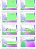 |
Fig. A.1 Kippenhahn diagram for different model sequences. The sequence number is shown in each diagram. Convective and overshooting layers are marked by green and yellow hatched lines, respectively. Semi-convective layers are marked by red dots. The net amount of energy loss and gain is indicated by color shading. The surface of the star is marked by a black solid line. |
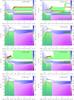 |
Fig. A.1 continued. |
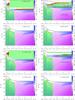 |
Fig. A.1 continued. |
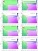 |
Fig. A.1 continued. |
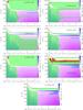 |
Fig. A.1 continued. |
 |
Fig. A.1 continued. |
In some model sequences, the convective layers in the hydrogen envelope during the late evolutionary stages look very noisy (m20vk02, m60vk02, and m15vk04). This is because the onset of convection depends sensitively on a minute change of the chemical gradient that is present in these layers. This phenomenon is frequently observed in massive star models.
Note that in this figure, we use the values on the ZAMS for rotational velocity and mass (i.e., vZAMS and MZAMS) given in Table 1, instead of the initial values.
Note added in proof: a paper by Chatzopoulos & Wheeler (2012) has recently been posted on astro-ph. Their result on the mass range for pair instability supernovae from rotating Pop III stars agrees well with ours.
Explosions as an energetic supernova without making a GRB might be another possibility for a star in this regime, as implied by the numerical studies of Burrows et al. (2007) and Dessart et al. (2008) on magnetically driven explosions caused by the magneto-rotational instability during core-collapse.
Acknowledgments
We are grateful to the anonymous referee for many invaluable criticisms, which have led to a significant improvement of the paper.
References
- Abel, T., Bryan, G., & Norman, M. L. 2000, ApJ, 540, 39 [NASA ADS] [CrossRef] [Google Scholar]
- Alexander, D. R., & Ferguson, J. W. 1994, ApJ, 437, 879 [NASA ADS] [CrossRef] [Google Scholar]
- Arlt, R., & Rüdiger, G. 2011, MNRAS, 412, 107 [NASA ADS] [CrossRef] [Google Scholar]
- Baraffe, I., Heger, A., & Woosley, S. E. 2005, ApJ, 550, 890 [Google Scholar]
- Bardeen, J. M., Press, W. H., & Teukolsky, S. A. 1972, ApJ, 178, 347 [NASA ADS] [CrossRef] [Google Scholar]
- Beers, T. C., & Christlieb, N. 2005, ARA&A, 43, 531 [NASA ADS] [CrossRef] [Google Scholar]
- Braithwaite, J. 2006, A&A, 449, 451 [NASA ADS] [CrossRef] [EDP Sciences] [Google Scholar]
- Bromm, V., Coppi, P. S., & Larson, R. B. 1999, ApJ, 527, L5 [NASA ADS] [CrossRef] [PubMed] [Google Scholar]
- Bromm, V., Yoshida, N., Hernquist, L., & McKee, C. F. 2009, Nature, 459, 49 [NASA ADS] [CrossRef] [PubMed] [Google Scholar]
- Brott, I., de Mink, S. E., & Cantiello, M., et al. 2011a, A&A, 530, A115 [NASA ADS] [CrossRef] [EDP Sciences] [Google Scholar]
- Bucciantini, N., Quataert, E., Metzger, B. D., et al. 2009, MNRAS, 396, 2038 [NASA ADS] [CrossRef] [Google Scholar]
- Burrows, A., Dessart, L., Livne, E., Ott, C. D., & Murphy, J. 2007, ApJ, 664, 416 [NASA ADS] [CrossRef] [Google Scholar]
- Cayrel, R., Depagne, E., Spite, M., et al. 2004, A&A, 416, 1117 [NASA ADS] [CrossRef] [EDP Sciences] [Google Scholar]
- Caughlan, G. R., Fowler, W. A., Marris, M. J., & Zimmerman, B. A. 1984, Atomic Dat. Nuc. Dat. Tables, 32, 197 [Google Scholar]
- Chatzopoulos, E., & Wheeler, J. C. 2012, ApJ, 748, 42 [NASA ADS] [CrossRef] [Google Scholar]
- Chieffi, A., & Limongi, M. 2004, ApJ, 608, 405 [NASA ADS] [CrossRef] [Google Scholar]
- Christlieb, N., Bessell, M. S., Beers, T. C., et al. 2002, Nature, 419, 904 [NASA ADS] [CrossRef] [PubMed] [Google Scholar]
- Cooke, R., Pettini, M., Steidel, C. C., Rudei, G. C., & Jorgenson, R. A. 2011, MNRAS, 412, 1047 [NASA ADS] [Google Scholar]
- Cucchiara, A., Levan, A. J., Fox, D. B., et al. 2011, ApJ, 736, 7 [NASA ADS] [CrossRef] [Google Scholar]
- Decressin, T., Meynet, G., Charbonnel, C., Prantzos, N., & Ekström, S. 2007, A&A, 464, 1029 [NASA ADS] [CrossRef] [EDP Sciences] [Google Scholar]
- de Mink, S. E., Pols, O. R., Langer, N., & Izzard, R. G. 2009, A&A, 501, L1 [NASA ADS] [CrossRef] [EDP Sciences] [Google Scholar]
- Denissenkov, P. A., & Herwig, F. 2003, ApJ, 590, L99 [NASA ADS] [CrossRef] [Google Scholar]
- Depagne, E., Hill, V., & Spite, M., et al. 2002, A&A, 390, 187 [NASA ADS] [CrossRef] [EDP Sciences] [Google Scholar]
- Dessart, L., Burrows, A., & Ott, C. D. 2008, ApJ, 673, L43 [NASA ADS] [CrossRef] [Google Scholar]
- Duncan, R. C., & Thompson, C. 1992, ApJ, 392, 9 [Google Scholar]
- Ekström, S., Meynet, G., Chiappini, C., Hirschi, R., & Maeder, A. 2008, A&A, 489, 685 [NASA ADS] [CrossRef] [EDP Sciences] [Google Scholar]
- Endal, A. S., & Sofia, S. 1976, ApJ, 210, 184 [NASA ADS] [CrossRef] [Google Scholar]
- Erni, P., Richter, P., Ledoux, C., & Petitjean, P. 2006, A&A, 451, 19 [NASA ADS] [CrossRef] [EDP Sciences] [Google Scholar]
- Foley, R. J., Smith, N., Ganeshalingam, M., et al. 2007, ApJ, 657, 105 [Google Scholar]
- Frebel, A., & Norris, J. E. 2011, Planets, Stars and Stellar Systems (Springer), 5, in press [arXiv:1102.1748v1] [Google Scholar]
- Gal-Yam, A., Mazzaili, P., Ofek, E. O., et al. 2009, Nature, 462, 624 [NASA ADS] [CrossRef] [PubMed] [Google Scholar]
- Gellert, M., Rüdiger, G., & Elstner, D. 2008, A&A, 479, L33 [NASA ADS] [CrossRef] [EDP Sciences] [Google Scholar]
- Glatzel, W., Fricke, K. J., & El Eid, M. 1985, A&A, 149, 413 [NASA ADS] [Google Scholar]
- Greiner, J., Krühler, T., Fynbo, J. P. U., et al. 2009, ApJ, 693, 1610 [NASA ADS] [CrossRef] [Google Scholar]
- Heger, A., & Woosley, S. E. 2002, ApJ, 567, 532 [NASA ADS] [CrossRef] [Google Scholar]
- Heger, A., & Woosley, S. E. 2010, ApJ, 724, 341 [NASA ADS] [CrossRef] [Google Scholar]
- Heger, A., Langer, N., & Woosley, S. E. 2000, ApJ, 528, 368 [NASA ADS] [CrossRef] [Google Scholar]
- Heger, A., Fryer, C. L., Woosley, S. E., Langer, N., & Hartmann, D. H. 2003, ApJ, 591, 288 [NASA ADS] [CrossRef] [Google Scholar]
- Heger, A., Woosley, S. E., & Spruit, H. 2005, ApJ, 626, 350 [NASA ADS] [CrossRef] [Google Scholar]
- Hirschi, R. 2007, A&A, 461, 571 [NASA ADS] [CrossRef] [EDP Sciences] [Google Scholar]
- Iglesias, C. A., & Rogers, F. J. 1996, ApJ, 464, 943 [NASA ADS] [CrossRef] [Google Scholar]
- Johnson, J., & Bromm, V. 2006, MNRAS, 366, 247 [NASA ADS] [Google Scholar]
- Kandus, A., Kunze, K., & Tsagas, C. G. 2011, Phys. Rep., 505, 1 [NASA ADS] [CrossRef] [Google Scholar]
- Kasen, D., Woosley, S. E., & Heger, A. 2011, ApJ, 734, 102 [NASA ADS] [CrossRef] [Google Scholar]
- Kawai, N., Kosugi, G., & Aoki, K., et al. 2006, Nature, 440, 184 [NASA ADS] [CrossRef] [PubMed] [Google Scholar]
- Kippenhahn, R. 1974, in Late Stages of Stellar Evolution, ed. R. J. Taylor, & J. E. Hesser, IAU Symp., 66, 20 [Google Scholar]
- Kippenhahn, R., & Weigert, R. 1990, Stellar Structure and Evolution (Berlin: Springer) [Google Scholar]
- Kobayashi, C., Tominaga, N., & Nomoto, K. 2011, ApJ, 730, 14 [Google Scholar]
- Komissarov, S. S., & Barkov, M. V. 2010, MNRAS, 402, L25 [NASA ADS] [Google Scholar]
- Krtička, J., & Kubát, J. 2006, A&A, 446, 1039 [NASA ADS] [CrossRef] [EDP Sciences] [Google Scholar]
- Krtička, J., & Kubát, J. 2009, A&A, 493, 585 [NASA ADS] [CrossRef] [EDP Sciences] [Google Scholar]
- Krtička, J.,Owocki, S. P., & Meynet, G. 2011, A&A, 527, A84 [NASA ADS] [CrossRef] [EDP Sciences] [Google Scholar]
- Kudritzki, R. P. 2002, ApJ, 577, 389 [NASA ADS] [CrossRef] [Google Scholar]
- Kudritzki, R. P., Pauldrach, A., Puls, J., & Abbott, D. C. 1989, A&A, 219, 205 [NASA ADS] [Google Scholar]
- Lai, D. K., Bolte, M., Johnson, J. A., et al. 2008, ApJ, 681, 1524 [NASA ADS] [CrossRef] [Google Scholar]
- Langer, N. 1991, A&A, 252, 669 [NASA ADS] [Google Scholar]
- Langer, N. 1997, in Luminous Blue Variables: Massive Stars in Transition, ed. A. Nota, & H. Lamers (San Francisco: ASP), ASP Conf. Ser., 120, 83 [Google Scholar]
- Macfadyen, A., & Woosley, S. E. 1999, ApJ, 524, 262 [NASA ADS] [CrossRef] [Google Scholar]
- Maeder, A. 1989, A&A, 178, 159 [NASA ADS] [Google Scholar]
- Maeder, A., & Meynet, G. 2000a, A&A, 361, 159 [NASA ADS] [Google Scholar]
- Maeder, A., & Meynet, G. 2000b, ARA&A, 38, 143 [NASA ADS] [CrossRef] [Google Scholar]
- Marigo, P., Girardi, L., Choisi, C., & Wood, P. R. 2001, A&A, 371, 152 [NASA ADS] [CrossRef] [EDP Sciences] [Google Scholar]
- Marigo, P., Chiosi, C., & Kudritzki, R.-P. 2003, A&A, 399, 617 [NASA ADS] [CrossRef] [EDP Sciences] [Google Scholar]
- Meynet, G., & Maeder, A. 2002, A&A, 390, 561 [NASA ADS] [CrossRef] [EDP Sciences] [Google Scholar]
- Mészáros, P., & Rees, M. J. 2010, ApJ, 715, 967 [NASA ADS] [CrossRef] [Google Scholar]
- Muijres, L. E., Vink, J. S., de Koter, A., et al. 2012, A&A, 537, A37 [NASA ADS] [CrossRef] [EDP Sciences] [Google Scholar]
- Nakamura, F., & Umemura, M. 2001, ApJ, 548, 19 [NASA ADS] [CrossRef] [Google Scholar]
- Nieuwenhuijzen, H., & de Jager, C. 1990, A&A, 231, 134 [NASA ADS] [Google Scholar]
- Nugis, T., & Lamers, H. J. G. L. M. 2000, A&A, 360, 227 [NASA ADS] [Google Scholar]
- Ober, W. W., El Eid, M. F., & Fricke, K. J. 1983, A&A, 119, 61 [NASA ADS] [Google Scholar]
- Omukai, K., & Palla, F. 2003, ApJ, 589, 677 [NASA ADS] [CrossRef] [Google Scholar]
- Ohkubo, T., Nomoto, K., Umeda, H., Yoshida, N., & Tsuruta, S. 2009, ApJ, 706, 1184 [NASA ADS] [CrossRef] [Google Scholar]
- Petrovic, J., Langer, N., Yoon, S.-C., & Heger, A. 2005, A&A, 435, 247 [NASA ADS] [CrossRef] [EDP Sciences] [Google Scholar]
- Pastorello, A., Smartt, S. J., & Mattila, S., et al. 2007, Nature, 447, 829 [NASA ADS] [CrossRef] [PubMed] [Google Scholar]
- Prantzos, N., & Charbonnel, C. 2006, A&A, 458, 135 [NASA ADS] [CrossRef] [EDP Sciences] [Google Scholar]
- Quimby, R. M., Kulkarni, S. R., Kasliwal, M. M., et al. 2011, Nature, 474, 487 [NASA ADS] [CrossRef] [Google Scholar]
- Salvaterra, R., Della Valle, M., Campana, S., et al. 2009, Nature, 461, 1258 [NASA ADS] [CrossRef] [PubMed] [Google Scholar]
- Smith, N., Li, W., & Foley, R. J., et al. 2007, ApJ, 666, 1116 [NASA ADS] [CrossRef] [Google Scholar]
- Spruit, H. C. 1999, A&A, 349, 189 [NASA ADS] [Google Scholar]
- Spruit, H. C. 2002, A&A, 381, 923 [NASA ADS] [CrossRef] [EDP Sciences] [Google Scholar]
- Stacy, A., Bromm, V., & Loeb, A. 2011, MNRAS, 413, 543 [NASA ADS] [CrossRef] [Google Scholar]
- Suijs, M. P. L., Langer, N., Poelarends, A.-J., et al. 2008, A&A, 481, 87 [Google Scholar]
- Suwa, Y., & Ioka, K. 2011, ApJ, 726, 107 [NASA ADS] [CrossRef] [Google Scholar]
- Tanvir, N. R., Fox, D. B., Levan, A. J., et al. 2009, Nature, 461, 1254 [NASA ADS] [CrossRef] [PubMed] [Google Scholar]
- Toma, K., Sakamoto, T., & Mészáros, P. 2011, ApJ, 731, 127 [NASA ADS] [CrossRef] [Google Scholar]
- Umeda, H., & Nomoto, K. 2003, Nature, 422, 871 [NASA ADS] [CrossRef] [PubMed] [Google Scholar]
- Umeda, H., & Nomoto, K. 2005, ApJ, 619, 427 [NASA ADS] [CrossRef] [Google Scholar]
- van Marle, A. J., Langer, N., Yoon, S.-C., & García-Segura, G. 2008, A&A, 478, 769 [NASA ADS] [CrossRef] [EDP Sciences] [Google Scholar]
- Ventura, P., D’Antona, F., Mazzitelli, I., & Gratton, R. 2001, ApJ, 550, L65 [NASA ADS] [CrossRef] [Google Scholar]
- Vink, J., & de Koter, A. 2005, A&A, 442, 587 [NASA ADS] [CrossRef] [EDP Sciences] [Google Scholar]
- Vink, J., de Koter, A., & Lamers, H. J. G. L. M. 2001, A&A, 369, 574 [NASA ADS] [CrossRef] [EDP Sciences] [Google Scholar]
- Wheeler, J. C., Yi, I., Höflich, P., & Wang, L. 2000, ApJ, 537, 810 [NASA ADS] [CrossRef] [Google Scholar]
- Woosley, S. E. 1993, ApJ, 405, 273 [NASA ADS] [CrossRef] [Google Scholar]
- Woosley, S. E., & Weaver, T. A. 1995, ApJS, 101, 181 [NASA ADS] [CrossRef] [Google Scholar]
- Woosley, S. E., & Heger, A. 2006, ApJ, 637, 914 [NASA ADS] [CrossRef] [Google Scholar]
- Woosley, S. E., Blinnikov, S., & Heger, A. 2007, Nature, 450, 390 [NASA ADS] [CrossRef] [PubMed] [Google Scholar]
- Yoon, S.-C., & Cantiello, M. 2010, ApJ, 717, L62 [NASA ADS] [CrossRef] [Google Scholar]
- Yoon, S.-C., & Langer, N. 2005, A&A, 443, 643 [NASA ADS] [CrossRef] [EDP Sciences] [Google Scholar]
- Yoon, S.-C., Langer, N., & Norman, C. 2006, A&A, 460, 199 [NASA ADS] [CrossRef] [EDP Sciences] [Google Scholar]
- Yoon, S.-C., Woosley, S. E., & Langer, N. 2010, ApJ, 725, 940 [NASA ADS] [CrossRef] [Google Scholar]
- Yoshida, N., Omukai, K., & Hernquist, L. 2007, ApJ, 667, 117 [Google Scholar]
- Zahn, J.-P., Brun, A. S., & Mathis, S. 2007, A&A, 474, 145 [NASA ADS] [CrossRef] [EDP Sciences] [Google Scholar]
All Tables
Initial conditions for the rotating model sequences, and the corresponding values on the zero-age main sequence (ZAMS).
Total energy (E), total number (N), and average wavelength () of the ionizing photons for hydrogen (H), neutral helium (He) and singly ionized helium (He+) during the evolution for each model sequence.
Yields in the last calculated model for each model sequence, in units of solar mass.
All Figures
|
Fig. 1 Evolution of the models in the HR diagram for 10, 15, 20, 30, 60 and 100 M⊙. Evolutionary tracks for different initial rotational velocities at a given initial mass are given in each panel as indicated by the labels. The end points of core hydrogen burning and core helium burning are marked by an square and a cross, respectively, on each evolutionary track. |
| In the text | |
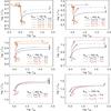 |
Fig. 2 Same as in Fig. 1, but for 150, 200, 250, 300, 500, and 1000 M⊙. |
| In the text | |
|
Fig. 3 Evolution of the central temperature and density in some model sequences for vinit/vK = 0 (upper panel) and vinit/vK = 0.6 (lower panel). The initial masses are marked by the labels in the figures. The regime for the pair-instability is marked by pink shading. |
| In the text | |
|
Fig. 4 Rotational velocity in units of the critical velocity (vcrit) given by Eq. (2) as a function of time for model sequences with Minit = 30, 100, 200, and 500 M⊙. The initial rotational velocity in units of the Keplerian value (vK) is indicated by the labels. Note that |
| In the text | |
|
Fig. 5 Mean specific angular momentum over the shells as a function of the mass coordinate at different evolutionary epochs (ZAMS, TAMS, core helium exhaustion, and the last calculated model) in Seqs. m30vk02, m30vk06, m200vk06 and m500vk04, as indicated by the labels. The thin sold line labeled jKerr,lso denotes the specific angular momentum for the last stable orbit at the given mass of a black hole, assuming that all mass below forms a rotating black hole. Here, if the contained angular momentum is higher than that of a maximally rotating black hole, the black hole is assumed to rotate maximally. |
| In the text | |
|
Fig. 6 Specific angular momentum as a function of the mass coordinate in the initial models with vinit/vK = 0.6 for different initial masses (20, 60, 100, 150, 200 and 250 M⊙) as indicated by the labels. |
| In the text | |
|
Fig. 7 Ratio of the total number of ionizing photons from non-rotating models to that from rotating models with vinit/vK = 0.4. The connecting lines of filled circles, triangles and squares give the values for hydrogen and first and second helium ionization, respectively. |
| In the text | |
|
Fig. 8 Kippenhahn diagram for Seq. m500vk00, which is same as in Fig. A.1 but zoomed up for 200 ≤ Mr/M⊙ ≤ 350, and 4.0 ≤ log (tf − t) ≤ 5.7. Here tf is the evolutionary time at the end of calculation. |
| In the text | |
|
Fig. 9 Mass fraction of different isotopes in the last model of Seq. m500vk00. |
| In the text | |
|
Fig. 10 Total yields of nitrogen as a function of the initial mass for vinit/vK = 0.0 (star symbol), 0.2 (open circle) and 0.4 (filled circle). For vinit/vK = 0.4, the CHE models are marked with a yellow color, while the NE/TE models with a purple color. The connecting line with open triangles gives the nitrogen yields of the rotating models by Ekström et al. (2008). |
| In the text | |
|
Fig. 11 Mass fraction of different isotopes in Seq. m30vk04, when primary nitrogen is abundantly produced during core helium burning. |
| In the text | |
|
Fig. 12 Phase diagram for the final fates of massive Pop III stars, in the plane of the mass and the fraction of the Keplerian value of the equatorial rotational velocity on the zero-age main sequence. The dotted line denotes the limit above which the rotational velocity at the surface would exceed the critical rotation velocity (vcrit in Eq. (2)). The thick solid line marks the boundary between the regimes for the chemically homogeneous evolution (CHE), and the non-CHE evolution (normal evolution or transitionary evolution; see Sect. 3). The regions for different final fates are divided by thin solid lines. Each acronym has the following meaning. SN IIP: Type IIP supernova, NS: neutron star, BH: black hole, SN II: type II supernova, PISN: pair-instability supernova, Puls. PISN: pulsational pair-instability supernova, GRB: gamma-ray bursts, HN: hypernova, SNIbc: type Ib or Ic supernova. |
| In the text | |
|
Fig. 13 τES,K in Eq. (8), divided by the main sequence lifetime (tMS) and multiplied by 1000, as a function of the initial mass. The ZAMS models of 20, 30, 60, 100, 250 and 500 M⊙ were used for the evaluation of τES,K. |
| In the text | |
|
Fig. 14 Upper panel: the evolution of τES,0/τES,K (see Eqs. (8) and (9)) in the model sequences m30vk03, m100vk04, m250vk04 and m500vk04. Only main sequence models are considered here. Bottom panel: the evolution of τES/τES,0 (see Eqs. (9) and (10)) in the corresponding model sequences. |
| In the text | |
|
Fig. 15 Mass fraction of helium at the surface (Ys) as a function of the mass fraction of helium at the center (Yc) during the main sequence for model sequences m30vk04, m250vk04 and m500vk04. The thin dotted line corresponds to the case of perfect chemical homogeneity. |
| In the text | |
|
Fig. A.1 Kippenhahn diagram for different model sequences. The sequence number is shown in each diagram. Convective and overshooting layers are marked by green and yellow hatched lines, respectively. Semi-convective layers are marked by red dots. The net amount of energy loss and gain is indicated by color shading. The surface of the star is marked by a black solid line. |
| In the text | |
|
Fig. A.1 continued. |
| In the text | |
|
Fig. A.1 continued. |
| In the text | |
|
Fig. A.1 continued. |
| In the text | |
|
Fig. A.1 continued. |
| In the text | |
|
Fig. A.1 continued. |
| In the text | |
Current usage metrics show cumulative count of Article Views (full-text article views including HTML views, PDF and ePub downloads, according to the available data) and Abstracts Views on Vision4Press platform.
Data correspond to usage on the plateform after 2015. The current usage metrics is available 48-96 hours after online publication and is updated daily on week days.
Initial download of the metrics may take a while.