| Issue |
A&A
Volume 540, April 2012
|
|
|---|---|---|
| Article Number | A123 | |
| Number of page(s) | 18 | |
| Section | Cosmology (including clusters of galaxies) | |
| DOI | https://doi.org/10.1051/0004-6361/201118697 | |
| Published online | 09 April 2012 | |
Multimodality in galaxy clusters from SDSS DR8: substructure and velocity distribution⋆
1 Tartu Observatory, 61602 Tõravere, Estonia
e-mail: This email address is being protected from spambots. You need JavaScript enabled to view it.
2 Tuorla Observatory, University of Turku, Väisäläntie 20, Piikkiö, Finland
3 National Institute of Chemical Physics and Biophysics, 10143 Tallinn, Estonia
4 Institute of Physics, Tartu University, Tähe 4, 51010 Tartu, Estonia
5 Estonian Academy of Sciences, 10130 Tallinn, Estonia
6 ICRANet, Piazza della Repubblica 10, 65122 Pescara, Italy
7 Observatori Astronòmic, Universitat de València, Apartat de Correus 22085, 46071 València, Spain
Received: 21 December 2011
Accepted: 19 February 2012
Abstract
Context. The study of the signatures of multimodality in groups and clusters of galaxies, an environment for most of the galaxies in the Universe, gives us information about the dynamical state of clusters and about merging processes, which affect the formation and evolution of galaxies, groups and clusters, and larger structures – superclusters of galaxies and the whole cosmic web.
Aims. We search for the presence of substructure, a non-Gaussian, asymmetrical velocity distribution of galaxies, and large peculiar velocities of the main galaxies in clusters with at least 50 member galaxies, drawn from the SDSS DR8.
Methods. We employ a number of 3D, 2D, and 1D tests to analyse the distribution of galaxies in clusters: 3D normal mixture modelling, the Dressler-Shectman test, the Anderson-Darling and Shapiro-Wilk tests, as well as the Anscombe-Glynn and the D’Agostino tests. We find the peculiar velocities of the main galaxies, and use principal component analysis to characterise our results.
Results. More than 80% of the clusters in our sample have substructure according to 3D normal mixture modelling, and the Dressler-Shectman (DS) test shows substructure in about 70% of the clusters. The median value of the peculiar velocities of the main galaxies in clusters is 206 km s-1 (41% of the rms velocity). The velocities of galaxies in more than 20% of the clusters show significant non-Gaussianity. While multidimensional normal mixture modelling is more sensitive than the DS test in resolving substructure in the sky distribution of cluster galaxies, the DS test determines better substructure expressed as tails in the velocity distribution of galaxies (possible line-of-sight mergers). Richer, larger, and more luminous clusters have larger amount of substructure and larger (compared to the rms velocity) peculiar velocities of the main galaxies. Principal component analysis of both the substructure indicators and the physical parametres of clusters shows that galaxy clusters are complicated objects, the properties of which cannot be explained with a small number of parametres or delimited by one single test.
Conclusions. The presence of substructure, the non-Gaussian velocity distributions, as well as the large peculiar velocities of the main galaxies, shows that most of the clusters in our sample are dynamically young.
Key words: large-scale structure of Universe / Galaxies: clusters: general
Tables 3 and 4 are available in electronic form at http://www.aanda.org
© ESO, 2012
1. Introduction
Most galaxies in the Universe are located in groups and clusters of galaxies, which themselves reside in larger systems – in superclusters of galaxies or in filaments crossing underdense regions between superclusters (Jõeveer et al. 1978; Gregory & Thompson 1978; Zeldovich et al. 1982; de Lapparent et al. 1986). In the ΛCDM concordance cosmological model the structures forming the cosmic web grow by hierarchical clustering driven by gravity (see, e.g., Loeb 2002, 2008, and references therein). The present-day dynamical state of clusters of galaxies depends on their formation history. Signatures of multimodality in the distribution of galaxies in clusters (the presence of substructure, several galaxy associations within clusters, non-Gaussian velocity distributions of galaxies, and large peculiar velocities of the main galaxies) are indicators of former or ongoing mergers in groups and clusters, which affect the formation and evolution of galaxies (Bird & Beers 1993; Pinkney et al. 1996; Knebe & Müller 2000). These mergers have shaped the properties of galaxies in groups and clusters, as, e.g., the well-known morphological segregation effect (Einasto et al. 1974; Dressler 1980; Einasto & Einasto 1987; Berrier et al. 2009; Huertas-Company et al. 2009). Substructure affects estimates of several cluster characteristics, the dynamical mass and mass-to-light ratio among others (Biviano et al. 2006; Niemi et al. 2007; Piffaretti & Valdarnini 2008; Holopainen et al. 2008; White et al. 2010; Power et al. 2011, and references therein). Detailed knowledge of the properties of clusters of galaxies is needed for comparison of observations with N-body models of the formation and evolution of cosmic structures, to test the cosmological models (Thomas et al. 1998; Araya-Melo et al. 2009).
To search for signatures of multimodality in galaxy clusters a number of 3D, 2D, and 1D methods have been proposed, including the Dressler-Shectman test (Dressler & Shectman 1988; Knebe & Müller 2000), the hierachical clustering method (Serna & Gerbal 1996; Durret et al. 2010), wavelet analysis (Flin & Krywult 2006), multidimensional normal mixture modelling (Fraley & Raftery 2006), see also Einasto et al. (2010), and many others (see Pinkney et al. 1996, for a review). Pinkney et al. (1996) showed that it is preferable to use several methods to search for substructure in clusters, since their sensitivity to different signatures of multimodality is different.
Several studies have shown the presence of substructure in poor and rich groups and clusters of galaxies (Solanes et al. 1999; Oegerle & Hill 2001; Kolokotronis et al. 2001; Burgett et al. 2004; Boschin et al. 2006; Flin & Krywult 2006; Barrena et al. 2007; Hwang & Lee 2007; Boschin et al. 2008; Hou et al. 2009; Vennik & Hopp 2009; Aguerri & Sánchez-Janssen 2010; Pimbblet et al. 2011; Ribeiro et al. 2011; Martínez & Zandivarez 2012; Hou et al. 2012), and in X-ray clusters (Ramella et al. 2007; Owers et al. 2009b,a; Böhringer et al. 2010; Andrade-Santos et al. 2012). Tovmassian & Plionis (2009) studied the properties of poor groups from the SDSS survey and showed that many groups of galaxies are not presently in a dynamical equilibrium, but at various stages of virialization. Niemi et al. (2007) showed that a significant fraction of nearby groups of galaxies are not even gravitationally bound systems.
In this paper we study the multimodality in rich clusters drawn from the SDSS DR8. We use data about 109 clusters with at least 50 member galaxies, this is one of the largest samples of rich clusters analysed for substructure so far. We employ a number of 3D, 2D, and 1D methods to analyse the distribution of galaxies in clusters. With the principal component analysis we characterise the results of different tests simultaneously, and study the relations between the multimodality of clusters and their physical properties. We present lists of unimodal and multimodal clusters. In Sect. 2 we describe the data we used. In Sect. 3 we describe the methods to search for signatures of multimodality, and we apply them in Sect. 4 to study the properties of clusters. We discuss the results and draw conclusions in Sect. 5.
We assume the standard cosmological parametres: the Hubble parametre H0 = 100 h km s-1 Mpc-1, the matter density Ωm = 0.27, and the dark energy density ΩΛ = 0.73.
2. Data
We used the MAIN galaxy sample of the 8th data release of the Sloan Digital Sky Survey (Aihara et al. 2011) with the apparent r magnitudes r ≤ 17.77, and the redshifts 0.009 ≤ z ≤ 0.200, in total 576 493 galaxies. We corrected the redshifts of galaxies for the motion relative to the CMB and computed the co-moving distances (Martínez & Saar 2002) of galaxies. The absolute magnitudes of galaxies were determined in the r-band (Mr) with the k-corrections for the SDSS galaxies, calculated using the KCORRECT algorithm (Blanton et al. 2003a; Blanton & Roweis 2007). In addition, we applied evolution corrections, using the luminosity evolution model of Blanton et al. (2003b). The magnitudes correspond to the rest-frame at the redshift z = 0. More details on similar data reduction for the SDSS DR7 can be found in Tago et al. (2010, hereafter T10).
We determine groups of galaxies using the Friends-of-Friends (FoF) cluster analysis method introduced in cosmology by Turner & Gott (1976); Zeldovich et al. (1982); Huchra & Geller (1982), and modified in Tago et al. (2008) and in T10. A galaxy belongs to a group of galaxies if this galaxy has at least one group member galaxy closer than a linking length. In a flux-limited sample the density of galaxies slowly decreases with distance. To take this selection effect into account properly when constructing a group catalogue from a flux-limited sample, we rescaled the linking length with distance, calibrating the scaling relation by observed groups (see T10 for details). As a result, the maximum sizes in the sky projection and the velocity dispersions of our groups are similar at all distances. This shows that distance-dependent selection effects have been properly accounted for. Our catalogue contains 77858 groups with at least 2 member galaxies. The richest groups in our catalogue correspond to rich clusters of galaxies. The details and availablility of the group catalogue based on SDSS DR8 are described in Tempel et al. (2012).
In flux-limited samples galaxies outside the observational window remain unobserved. To calculate the total luminosities of groups we have to take into account the luminosities of these galaxies as well. For that, we multiply the observed galaxy luminosities by the luminosity weight Wd. The distance-dependent weight factor Wd was calculated as follows: 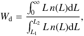 (1)where L1,2 = L⊙100.4(M⊙ − M1,2) are the luminosity limits of the observational window at a distance d, corresponding to the absolute magnitude limits of the survey M1 and M2; we took M⊙ = 4.64 mag in the r-band (Blanton & Roweis 2007), and n(L) is the galaxy luminosity function. Owing to their peculiar velocities, the distances of galaxies are somewhat uncertain; if the galaxy belongs to a group, we used the group distance (mean distance of galaxies in a group) to determine the weight factor. Detailed description, how the weight factor and luminosity function are calculated can be found in Tempel et al. (2011).
In the group catalogue the main galaxy of a group is defined as the most luminous galaxy in the r-band. We use this definition also in the present paper.
Next we select clusters for this study. The larger the number of galaxies in clusters, the more reliable is the analysis of substructure and their velocity distribution. Aguerri & Sánchez-Janssen (2010) select clusters with at least 30 member galaxies for substructure study. However, Boschin et al. (2008) argue that clusters with about 30 member galaxies are too small for the analysis of substructure (see also the discussion about the substructure statistics in small samples in Biviano et al. 2006), although clusters with smaller numbers of galaxies have been studied for substructure (see, for example, Solanes et al. 1999; Boschin et al. 2008; Ribeiro et al. 2011). Another problem arises with the selection effects: in the group catalogue the richness of groups decreases rapidly at distances D > 340 h-1Mpc owing to the use of a flux-limited sample of galaxies (T10). At distances smaller than 120 h-1Mpc the sample includes nearby exceptionally rich clusters which correspond to well-known Abell clusters (the Coma cluster, rich clusters in the Hercules supercluster and others, see T10 and Einasto et al. 2011b). These clusters have to be analysed separately. Therefore we chose for the present analysis clusters with at least 50 member galaxies in the distance interval 120 h-1Mpc ≤ D ≤ 340 h-1Mpc (redshift interval 0.04 ≤ z ≤ 0.12). This sample includes all clusters from the SDSS DR8 with at least 50 member galaxies from our catalogue in this distance interval, in total 109 clusters. Figure 1 shows the richness of clusters in our sample vs. their distance.
We cross-identify groups with Abell clusters, which have acquired a role of a reference system for rich clusters. Contrary to expectations, cross-identification of (rich) SDSS DR8 groups with Abell clusters is not straightforward. Problems arise both due to different group/cluster finding procedures as well as different algorithms for components/subgroups. The Abell clusters have a constant linear radius (1.5 h-1Mpc), while the DR8 groups obtained by a FoF procedure have various linear sizes. An Abell cluster may consist of several subclusters and/or may be the result of projections of groups from different distance (e.g. Pimbblet et al. 2011). These facts make cross-identification difficult. We consider a group identified with an Abell cluster, if the distance between their centres is smaller than at least the linear radius of one of the clusters, and the distance between their centres in the radial (line-of-sight) direction is less than 600 km s-1 (an empirical value). As a result one group can be identified with more than one Abell clusters and vice versa. This can be seen in Tables 3 and 4, where we give data on the clusters, and the results of the tests. In Fig. 2 we show the distributions of cluster redshifts and total luminosities, as given in Table 3.
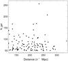 |
Fig. 1 Richness of clusters vs. their distance. |
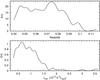 |
Fig. 2 Distribution of cluster redshifts (upper panel) and total luminosities (lower panel). |
3. Methods
In this section we decribe the methods applied in this paper to analyse the multimodality of galaxy clusters.
3.1. Multidimensional normal mixture modelling with Mclust
To search for possible components in clusters, we employ multidimensional normal mixture modelling based on the analysis of a finite mixture of distributions, in which each mixture component is taken to correspond to a different group, cluster or subpopulation. The most common component distribution considered in model-based clustering is a multivariate Gaussian (or normal) distribution. To model the collection of components, we apply the Mclust package for classification and clustering (Fraley & Raftery 2006) from R, an open-source free statistical environment developed under the GNU GPL (Ihaka & Gentleman 1996, http://www.r-project.org). This package searches for an optimal model for the clustering of the data among models with varying shape, orientation and volume, finds the optimal number of components, and the corresponding classification (the membership of each component). Mclust calculates for every galaxy the probabilities to belong to any of the components. The uncertainty of classification is defined as one minus the highest probability of a galaxy to belong to a component. The mean uncertainty for the full sample is used as a statistical estimate of the reliability of the results.
We tested how the possible errors in the line-of-sight positions of galaxies affect the results of Mclust, shifting randomly the peculiar velocities of galaxies 1000 times and searching each time for the components with Mclust. The random shifts were chosen from a Gaussian distribution with the dispersion equal to the sample velocity dispersion of galaxies in a cluster. The number of the components found by Mclust remained unchanged, demonstrating that the results of Mclust are not sensitive to such errors.
We also performed substructure analysis with Mclust using only the sky coordinates of the clusters as an additional 2D test.
3.2. DS test
Another diagnostic for substructure in clusters is the Dressler-Shectman (DS or Δ) test (Dressler & Shectman 1988). The DS test searches for deviations of the local velocity mean and dispersion from the cluster mean values. The algorithm starts by calculating the mean velocity (vlocal) and the velocity dispersion (σlocal) for each galaxy of the cluster, using its n nearest neighbours. These values of local kinematics are compared with the mean velocity (vc) and the velocity dispersion (σc) determined for the entire cluster of Ngal galaxies. The differences between the local and global kinematics are quantified by
![Mathematical equation: $$ \delta_i^2 = (n+1)/\sigma_{\rm c}^2\left[(v_\mathrm{local}-v_{\rm c})^2 + (\sigma_\mathrm{local}-\sigma_{\rm c})^2\right]. $$](/articles/aa/full_html/2012/04/aa18697-11/aa18697-11-eq32.png) The cumulative deviation Δ = Σδi is used as a statistic for quantifying (the significance of) the substructure. The results of the DS-test depend on the number of local galaxies n. Here, we have studied the substructure by using
The cumulative deviation Δ = Σδi is used as a statistic for quantifying (the significance of) the substructure. The results of the DS-test depend on the number of local galaxies n. Here, we have studied the substructure by using  , as suggested by Pinkney et al. (1996).
If the cluster velocity distribution is close to a Gaussian, then Δ will be of order Ngal. For the case of non-Gaussian velocities, Δ can differ significantly from Ngal, even if there is no subclustering (Dressler & Shectman 1988). Therefore, the Δ statistic for each cluster should be calibrated by Monte Carlo simulations. In Monte Carlo models the velocities of galaxies are randomly shuffled among the positions, which effectively destroys any true correlation between the velocities and positions. We ran 25 000 models for each cluster and calculated every time Δsim. The significance of having substructure (the p-value) can be quantified by the ratio N(Δsim > Δobs)/Nsim – the ratio of the number of simulations in which the value of Δ is larger than the observed value, and the total number of simulations. The smaller the p-value, the larger is the probability of substructure.
3.3. α test
With the α test developed by West & Bothun (1990) we analyse correlations between positions and velocities of galaxies and search for a region which differs from the overall distribution. This test gives a measure of the centroid shift for the cluster galaxies. The idea of the test is to search for a region that shows correlation between the positions and velocities that differs from that for the overall galaxy distribution. The method consists of a five different steps. At first the centroid of the system (xc,yc) is calculated as a global mean value. Next each galaxy i gets a weight wi = 1/Vi, where Vi is the line-of-sight rms velocity calculated using the velocities of the galaxy and its 10 nearest members. For each galaxy 10 nearest neighbours are chosen in the velocity space and new centroid (xc′,yc′) is calculated using the weights: 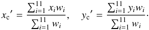 (2)In the fourth step it is calculated how much this new centroid differs from the global centroid:
  (3)Finally the average value of αi for all galaxies is defined as the α-value. This is a measure of how much the centroid of all galaxies shifts as a result of local correlations between the positions and velocities of galaxies.
3.4. β test
We also employ 2D tests which use information about the sky positions of galaxies in clusters: the β test which studies the asymmetry in the galaxy distribution (West et al. 1988) and 2D normal mixture modelling with Mclust.
The β test, presented in West et al. (1988), is a test for the asymmetry in the galaxy distribution. At first, the mean distance di for each galaxy i to its five nearest neighbours is calculated. Then a point diametrically opposite to this point is chosen and the mean distance do in this neighbourhood is calculated as before. The asymmetry is then measured by the β-value:  (4)To evaluate the asymmetry the average value ⟨ β ⟩ over all galaxies is calculated and any deviation from ⟨ β ⟩ ≈ 0 signifies asymmetry and possible substructure. According to Pinkney et al. (1996) the β test is sensitive to the mirror asymmetry, but not to the deviations from the radial symmetry. The p-values for the α and β tests are calculated with Monte Carlo simulations as for the DS test using 25 000 random sampling of galaxy coordinates in clusters.
3.5. 1D tests
One indicator of multimodality in clusters is the deviation of the distribution of the galaxy velocities in clusters from a Gaussian. To analyse the distribution of the velocities of galaxies we use several 1D tests. We tested the hypothesis about the Gaussian distribution of the peculiar velocities of galaxies in clusters with the Shapiro-Wilk normality test (Shapiro 1965), which is considered the best for small samples. We also employed the Anderson-Darling test, which is very reliable according to Hou et al. (2009). We calculated the kurtosis and the skewness of the peculiar velocity distributions, and used these to test for the asymmetry of the distributions of galaxy velocities. We used the Anscombe-Glynn test for the kurtosis (Anscombe & Glynn 1983), and the D’Agostino test for the skewness (D’Agostino 1970), from the R package moments by Komsta and Novomestky.
There is, of course, no reason to assume that the velocity distributions in galaxy clusters should be exactly Gaussian. In fact, kinematic models show that the shape of the velocity distribution is defined by the ratio of different types of galaxy orbits (Merritt 1987). The tests described above serve mostly to check if the velocity distribution is unimodal and symmetrical. Historically, they have been selected because of the easy availability of statistical tests for the Gaussian distribution; we use them to be able to compare our results with those obtained earlier.
In virialized clusters galaxies follow the cluster potential well. If so, we would expect that the main galaxies in clusters lie at the centres of groups (group haloes) and have small peculiar velocities (Ostriker & Tremaine 1975; Merritt 1984; Malumuth 1992). Therefore the peculiar velocity of the main galaxies in clusters is also an indication of the dynamical state of the cluster (Coziol et al. 2009). We calculate the peculiar velocities of the main galaxies, |Vpec|, the normalised peculiar velocities of the main galaxies, Vpec,r = |Vpec|/σv, and analyse the location of the main galaxies in the clusters and subclusters.
3.6. Principal component analysis
We employ the principal component analysis (PCA) to analyse the results of all tests simultaneously, and to study the relations between the multimodality indicators and the physical parametres of clusters. The aim of the PCA is to study the relations between the parametres and, if possible, to find a small number of linear combinations of correlated parametres to describe most of the variation in the dataset with a small number of new uncorrelated parametres. The PCA transforms the data to a new coordinate system, where the greatest variance by any projection of the data lies along the first coordinate (the first principal component), the second greatest variance – along the second coordinate, and so on. There are as many principal components as there are parametres, but often only the first few are needed to explain most of the total variation.
The principal components PCi (i ∈ N, i ≤ Ntot) are linear combinations of the original parametres:
 (5)where − 1 ≤ a(k)i ≤ 1 are the coefficients of the linear transformation, Vk are the original parametres and Ntot is the number of the original parametres. In the analysis the parametres are standardised – they are centred on their means,
  , and normalised, divided by their standard deviations, σ(Vk). The PCA is suitable tool for exploratory data analysis, to study simultaneously correlations between a large number of parametres (see Einasto et al. 2011a, for references about applications of the PCA in astronomy).
4. Results
We show in Table 1 the numbers and fractions of clusters with substructure, and with the p-values showing statistically significant deviations from Gaussianity in their galaxy distributions (p ≤ 0.05).
Results of the tests.
Table 1 shows that more than 80% of the clusters in our sample have multiple components, as detected by Mclust by the 3D analysis. About 75% of the clusters continue to show multiple components, if we use only the sky distribution of galaxies. More than 70% of all the clusters and more than 75% of the multicomponent clusters show statistically significant substructure according to the DS test, also; these fractions are slightly smaller for the α and β tests. The fractions of clusters with non-Gaussian velocity distributions are much smaller. The reason is that in many clusters galaxies from different components in the sky coordinates have similar (nearly Gaussian) distributions of velocities (we will show below a few examples of that). One-component clusters show signatures of substructure and non-Gaussian velocity distributions according to the DS, α, and other tests as well, but as seen from Table 1, the fractions of such clusters are smaller than those for multicomponent clusters. There are three clusters for which pAD ≤ 0.05, but pSW ≥ 0.05, and eight clusters with pSW ≤ 0.05, but pAD ≥ 0.05. Hou et al. (2009) showed that the AD test is very reliable; in our study the SW test detected non-Gaussian velocity distributions in a larger number of clusters, but there are also clusters for which the AD test found significant non-Gaussianity in the velocity distributions of galaxies, but the SW test did not.
Comparison with other studies shows that Ramella et al. (2007) found substructure in 73% of X-ray clusters which is very close to what we found by 2D normal mixture modelling. Solanes et al. (1999), Oegerle & Hill (2001), and Aguerri & Sánchez-Janssen (2010) found with the DS test that 30–50% of clusters have significant substructure. Flin & Krywult (2006) detected substructure in about 1/3 of Abell clusters studied by them using wavelet analysis. About 20–30% of clusters have non-Gaussian velocity distributions, as shown with the AD test or other 1D tests (Solanes et al. 1999; Oegerle & Hill 2001; Hou et al. 2009; Ribeiro et al. 2011; Martínez & Zandivarez 2012).
4.1. Peculiar velocities of cluster main galaxies
Figure 3 shows the distributions of the peculiar velocities Vpec and normalised peculiar velocities Vpec,r of the main galaxy in clusters, separately for one-component and multicomponent clusters. The peculiar velocity and normalised peculiar velocity distributions for main galaxies of one-component clusters we see a maximum at velocities less than 250 km s-1 (0.5 for the normalised peculiar velocities), followed by another maximum at larger velocities. Checking the distributions of galaxies in the clusters shows that in these clusters where the main galaxy has a peculiar velocity less than 250 km s-1, it is located in a component close to the central part of the cluster. If the peculiar velocity is higher, the main galaxy is located at the edge of the cluster, in multicomponent clusters typically in another component.
Table 1 shows that in about half of the multicomponent clusters the peculiar velocity of main galaxy is larger than 250 km s-1 (0.5 for normalised peculiar velocities). There is a clear difference between the median values of the peculiar velocities and normalised peculiar velocities of the one-component and multicomponent clusters – these velocities are much larger in the multicomponent clusters. This agrees with the results of Coziol et al. (2009) who found that the median value of the normalised peculiar velocities of main galaxies in the Abell clusters is 0.32, which is between the values found in this study.
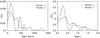 |
Fig. 3 Distribution of the peculiar velocities of main galaxies, Vpec (left panel), and the normalised peculiar velocities of main galaxies, Vpec,r (right panel), for clusters with one component (dashed line) and with multiple components (solid line). |
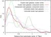 |
Fig. 4 Distribution of the distance of the main galaxy from the cluster (subcluster or component) centre for various subsamples of galaxies. Multicomponent clusters: grey dotted line – the distance of the main galaxy from the cluster centre; red solid line – the distance of the main galaxy from the (nearest) component centre; blue dashed line – the distance of the brightest galaxy in a component from the component centre. One-component clusters: dark green long-dashed line – the distance from the cluster centre; light green dotted-dashed line – the minimum distance of one of the three brightest galaxies from the cluster centre. |
Figure 4 shows the 2D distance of the main galaxy from the cluster centre, both for the multicomponent and one-component clusters. It is well seen that in multicomponent clusters a large fraction of main galaxies are located far away from the cluster centre (grey dotted line). However, when looking at the components found by 3D normal mixture modelling, we see that the main galaxies of clusters are preferentially located close to the centre of one of the components (red solid line). The distribution of distances from the component centre for the brightest galaxies in the components (Fig. 4) shows that these galaxies are also located preferentially close to the component centre (blue dashed line).
The distribution of the distances of the main galaxy from the cluster centre in one-component clusters (Fig. 4, dark green long-dashed line) shows that more than a half of the main galaxies are located near the cluster centre, but there is also a substantial number of main galaxies, which are further away from the cluster centre. We calculated also the minimum distance from the cluster centre for three brightest galaxies in the one-component clusters. As seen from Fig. 4 (light green dotted-dashed line), one of the three brightest galaxies in clusters is always located close to the cluster centre. This shows that the central galaxy of a cluster is typically one of the most luminous galaxies, but not always the most luminous one.
4.2. Comparison of the results of different tests
In Fig. 5 we compare the following properties of clusters: the number of components determined by the 3D version of Mclust, the peculiar and normalised peculiar velocities of main galaxies, and the Gaussianity of the velocity distribution of galaxies in clusters, as estimated by the Anderson-Darling and Shapiro-Wilk tests. Here we see that we have clusters consisting of up to eight components. The peculiar velocities of the main galaxies may be large both in the clusters with one component and with multiple components, as was seen also in Fig. 3. There are six clusters with five or more components, but only two of them have non-Gaussian velocity distributions of galaxies according to both tests (both are five-component clusters with Vpec ≈ 280 km s-1, so their symbols coincide in Fig. 5).
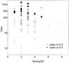 |
Fig. 5 Peculiar velocities of main cluster galaxies and the number of separate components in the clusters. Large symbols mark clusters with a non-Gaussian velocity distribution of galaxies (pAD < 0.05 and pSW < 0.05). Empty circles denote clusters with normalised peculiar velocities of their main galaxies Vpec,r < 0.5, filled circles denote clusters with Vpec,r > 0.5. |
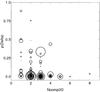 |
Fig. 6 3D tests: the Dressler-Shectman test p-value versus the number of components in a cluster. Symbol sizes are proportional to the peculiar velocities of main galaxies, Vpec. Small p-values show high probability of substructure. |
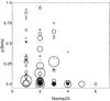 |
Fig. 7 2D tests: the number of cluster components versus the asymmetry (pβ). Symbol sizes are proportional to the peculiar velocities of main galaxies, Vpec. |
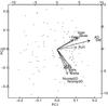 |
Fig. 8 Principal component analysis biplot for all tests. |
Results of the principal component analysis for the tests.
Figure 6 compares the results of the DS test and the 3D component analysis. Symbol sizes indicate the values of the peculiar velocities of the main galaxies in the clusters. Figure 6 shows that many multicomponent clusters, for which the DS test finds the presence of substructure, have large peculiar velocities of the main galaxes. There are seven one-component clusters after Mclust, for which the DS test suggests that these clusters have significant substructure (see also Table 1). Visual analysis of these clusters shows that these clusters have tails in their velocity distribution, and for some of these clusters the AD and/or SW tests also suggest a non-Gaussian distribution of galaxy velocities. There are 22 multicomponent clusters in our sample, which according to the DS test have no significant substructure. Our analysis showed that these clusters have components in the sky distribution of galaxies with similar distributions of velocities. Thus while Mclust finds better the components in the sky distribution of galaxies, the DS test is more sensitive to the possible substructure in the velocity distribution.
Figure 7 compares the results of the β test and the 2D component analysis with Mclust. The maximum number of components detected in the sky coordinates is slightly smaller than that found using both the sky coordinates and the velocities of galaxies. Figure 7 shows that there are multicomponent clusters without significant asymmetry (pβ > 0.05) and with large peculiar velocities of main galaxies (30 clusters). Comparison with the results of the DS test shows that 20 of these clusters have significant substructure, according to this test. There are 12 multicomponent clusters with significant asymmetry in the sky distribution of galaxies, according to the β test, but without significant substructure, according to the DS test, showing that the velocity distribution of galaxies in different cluster components is similar.
Next we will use the principal component analysis to compare the results of all tests simultaneously. We will use logarithmic scale for the peculiar velocities of main galaxies, this makes their range smaller. Figure 8 and Table 2 show the results of this analysis. In the biplot (Fig. 8) the arrows represent the axes where each original variable lies, and their length is proportional to their importance within each PC. In calculations we use 1 − p instead of the p-value – larger values of 1 − p suggest a higher probability to have substructure, therefore in this case the arrows corresponding to the number of the components in 3D and 2D point towards the same direction as the arrows corresponding to the DS, α, and β tests. The locations of clusters in the PC space are also plotted. In Table 2 we give the values of the principal components and the standard deviations, the proportion of variance, and the cumulative variance of the principal components. The values of the components show the importance of the original parametres in each PCi.
In Fig. 8 the arrows corresponding to the 3D and 2D tests are oriented towards about the same direction, the arrows corresponding to the 1D tests are pointed at a direction almost at the right angle to this, and form another set. This suggests that the results of the 3D and 2D tests are correlated, as well as the results of 1D tests among themselves. Among the 3D and 2D tests the highest importance in first two principal PCA components have the numbers of components determined with normal mixture modelling, followed by the DS test. The α and β tests are of almost equal importance. Among the 1D tests, the results of the Anderson-Darling and the Shapiro-Wilk tests have equal importance in determining the non-Gaussianity of the velocity distribution.
Table 2 shows that seven principal components are needed to explain more than 90% of the variance in the parametres, thus there is no one dominant test which could find most of the information about multimodality of the galaxy distribution in clusters.
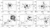 |
Fig. 9 Two of the most non-Gaussian clusters in our sample. Upper row: the cluster 34726 (Abell cluster A2028). Lower row: the cluster 914 (A1750). From left to right: the DS test bubble plot (here symbol sizes are proportional to the eδ), and RA vs. Dec, and RA vs. velocity (in 102 km s-1) plots; the symbols show different components as found by Mclust. The star marks the location of the main galaxy. |
Different types of clusters populate different regions in the PC1-PC2 plane. Unimodal clusters with Gaussian distribution of velocities are located in the upper lefthand part of the plot and have larger PC2 and larger negative PC1 values (for example, the clusters 608 and 58604). Multimodal clusters populate the lower righthand area of the biplot (the clusters 34727 and 914). Clusters with small values of the peculiar velocities of main galaxies, with a Gaussian distribution of velocities, but with a large number of components populate the lefthand lower area of the PC1-PC2 plane (the clusters 29348 and 4744). Multimodal clusters with large peculiar velocities of main galaxies and with non-Gaussian velocity distributions are located in the upper righthand area of the plane (the clusters 4122, 23374 and others).
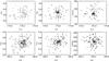 |
Fig. 10 Two of the most Gaussian clusters in our sample. Upper row: the cluster 58604. Lower row: the cluster 60539. From left to right: the DS test bubble plot (symbol sizes are proportional to the eδ), and RA vs. Dec, and RA vs. velocity (in 102 km s-1) plots; the symbols show different components as found by Mclust. The star marks the location of the main galaxy. |
4.3. Examples of multimodal and unimodal clusters
In our sample there are eight clusters which show signatures of non-Gaussianity in their galaxy distribution by all the tests. They have multiple components, the 3D and 2D tests confirm the presence of substructures and of asymmetry, and their velocity distributions differ from Gaussian at a very high statistical significance: the clusters 880, 4122, 28387, 34726, 58305, 67297, 68625, and 73088. Many clusters with multiple components are missing from this list, for example the cluster 914, a well-known binary merging Abell cluster A1750 in the Sloan Great Wall (Einasto et al. 2010, 2011c,b, and references therein), because in many multicomponent clusters galaxies from different components have similar distributions of velocities.
Figure 9 shows the distribution of galaxies in a cluster with four components, the cluster 34726, and in the cluster 914 with five components.
The cluster 34726 is one of the two clusters in our sample which can be identified with the Abell cluster A2028 in sky projection, another one is the cluster 34727. A2028 is a merging X-ray cluster with substructure (Flin & Krywult 2006; Gastaldello et al. 2010), which redshift close to the redshift of our cluster 34727. This is one example of projections in the Abell cluster catalogue. Figure 9 (upper row) shows that the sky distribution of galaxies in the cluster 34726 has two main components. In one of them the concentration of galaxies is especially high. This component is well seen in the distribution of velocities where very large velocity dispersion suggest a finger-of-god effect (right panel). Here also according to the DS test the probability of substructure is high. The α and β tests confirm the presence of substructure and asymmetry in the distribution of galaxies, the AD and SW tests show non-Gaussianity of the distribution of velocities of galaxies in this cluster. The peculiar velocity of the main galaxy is small.
The cluster 914 (Fig. 9, lower row) that corresponds to the Abell cluster A1750 is a well-known merging binary X-ray cluster (Donnelly et al. 2001; Belsole et al. 2004; Burgett et al. 2004; Hwang & Lee 2009; Einasto et al. 2010). In this cluster we see even five components. The DS test shows that the probability of substructure is the largest in the component where the main galaxy is located (Fig. 9, lower left panel). The peculiar velocity of the main galaxy is large. Other 3D and 2D tests confirm the presence of substructure and an asymmetrical galaxy distribution in A1750. Galaxies from different components in this cluster have similar velocity distributions, so according to the AD and SW tests their distribution is Gaussian (for details and references we refer also to Einasto et al. 2010).
Next we list the clusters for which all tests confirm unimodality and the Gaussian velocity distribution of galaxies: 608, 5217, 25078, 39914, 50129, 58604, and 67116. In Fig. 10 we plot the distribution of galaxies in two of them – in the cluster 58604, and in the cluster 60539 (A1516, the richest cluster in the supercluster SCl 111 in the Sloan Great Wall, described in Einasto et al. 2010). For the cluster 58604 all our tests confirm that this is an unimodal cluster. The peculiar velocity of the main galaxy is rather large for an unimodal cluster, about 200 km s-1. The cluster A1516 has the most regular ellipsoidal sky distribution of galaxies among the clusters in our sample, with a small peculiar velocity of the main galaxy. However, the distribution of velocities in the central part of the cluster shows an excess of negative (in respect of the cluster centre) velocities, and according to the DS and α tests this cluster may have substructure (see also an analysis of this cluster in Einasto et al. 2010). This may be a signature of a line-of-sight merger (see also Pinkney et al. 1996).
Results of the principal component analysis for the test results and for the physical parametres of clusters, combined.
In Tables A.1–A.4 we present the data about the most unimodal and most multimodal clusters, as well as data about the clusters with at least five components, and about those one-component clusters for which the DS test found significant substructure.
4.4. Non-Gaussianity parametres and physical properties of clusters
The principal component analysis can help us to study the relation between the physical parametres of clusters and the presence of substructure. In these calculations we include the number of components as determined with the 3D normal mixture modelling, the p-value for the DS test, pΔ, the peculiar velocity of the main galaxy in a cluster, Vpec, the number of galaxies in a cluster, Ngal, the total luminosity of a cluster, Ltot, the virial radius of a cluster, rvir, and the rms velocity of the cluster galaxies. We again use 1 − pΔ, and use logarithms of the peculiar velocities of main galaxies and of the physical parametres. Figure 11 and Table 3 show the results of this analysis.
In Fig. 11 the arrows corresponding to the tests for substructure and the arrows corresponding to the physical parametres of clusters do not point to the same direction – the correlations between the parametres are not strong, when we consider all parametres simultaneously. The coefficients of the first principal component in Table 3 show that the physical parametres are of larger importance than the substructure indicators. The coefficient corresponding to the luminosity of a cluster is the largest, but the differences between the values of the coefficients are not large, so there is no single dominant parametre. Among the coefficients of the second principal component the number of components has the largest (absolute) coefficient. Among the coefficients of the third principal component the peculiar velocities of the main galaxy, and the rms velocity of galaxies in a cluster are of equal importance. In Fig. 11 the arrow corresponding to the peculiar velocity of the main galaxy in a cluster points to the same direction as the arrow for the rms velocity of a cluster, showing that these velocities are larger in clusters with larger rms velocities. These clusters are also richer.
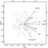 |
Fig. 11 Principal component analysis with Ncomp3D, Vpec, and pΔ, and the physical parametres of clusters (Ltot, Ngal, rvir, and rms velocity). |
Table 3 shows that the first principal component accounts for almost 38% of the variance of parametres. Five principal components are needed to explain more than 90% of the variance of the parametres – clusters are complicated objects, the properties of which cannot be explained with a small number of parametres (in contrast to superclusters which can be described with a small number of parametres, see Einasto et al. 2011a).
In the PC1-PC2 plane one-component clusters with a Gaussian distribution of velocities are located at the upper lefthand part of the plot and have larger PC2 and smaller (larger negative) PC1 values (for example, the clusters 608 and 28508). Multicomponent clusters of high luminosity populate the lower and middle righthand area of the biplot (the clusters 34727 and 914). Less luminous multicomponent clusters populate the lefthand lower area of the PC1- PC2 plane (the clusters 11474 and 11015). One-component clusters with large rms velocities of galaxies populate the upper righthand area of the plane (the clusters 16350, 17210, and others).
We checked for pairwise correlations between the physical parametres of clusters and the substructure characteristics and found that correlations between the number of galaxies in clusters, the total luminosity of clusters, the virial radius of clusters, and the numbers of components and the presence of substructure according to the 3D and 2D tests are statistically highly significant – richer, larger and more luminous clusters have a larger amount of substructure.
5. Discussion and conclusions
5.1. Comparison with other studies
An increasing number of studies have shown recently the presence of substructure in groups and clusters of galaxies determined using optical or X-ray data (see references in Sect. 1). We detected multiple components in more than 80% of the clusters using multidimensional normal mixture modelling. Comparison with other studies in Sect. 4 showed that although this is a higher fraction of multimodal clusters than found in other studies, comparison of the fractions of clusters with substructure or with non-Gaussian velocity distributions determined with similar methods gives the results in a good agreement with others. This supports our choice of the parametres for the FoF algorithm for group definition and suggests that in our catalogue groups with substructure are real groups and not complexes of small groups, artificially linked together by an unreasonable choise of linking parametres.
The fractions of clusters with substructure found in X-ray clusters by Ramella et al. (2007) is almost the same that we found with the 2D normal mixture modelling. In these studies there are eight common clusters; in seven of them substructure have been detected in both studies. Ramella et al. (2007) found two components in A602 (cluster 43545), this is unimodal cluster according to our calculations. In the sky distribution this cluster has a very elongated shape; this may be visible in X-rays as two components.
Comparison with Flin & Krywult (2006) shows that they detected substructures in all 14 clusters common for both studies; we found multiple components in 12 clusters. A1809 (our cluster 67116) is an unimodal cluster according to Mclust, although the DS and α tests detected substructure at the 90% significance level. We detected no substructure in A1650 (25078) while Flin & Krywult (2006) mention that there is one group of galaxies in the field of the galaxies in this cluster. Therefore, an overall agreement between the results of our study and Flin & Krywult (2006) is very good, considering that the sample selection and the methods to analyse modality of clusters are different.
The cluster A1750 (our cluster 914) has been studied for substructure by other authors, too. We mentioned above that the components found in this cluster by us coincide well with those found in other studies (see Einasto et al. 2010, for details). We found an especially good agreement between our results and those by Burgett et al. (2004) and Hwang & Lee (2009).
We have three common clusters with those searched for rotation by Hwang & Lee (2007). We found that all of them (A1035, A1139, and A2169; these are our clusters 20159, 3714, and 12508) are multimodal clusters which agrees with the results of the DS test by Hwang & Lee (2007). They also suggest that the clusters A1139 and A2169 may be rotating or merging. We have also five common clusters with those studied by Burgett et al. (2004) using data from the 2dFGRS. All of them (A1139, A1238, A1620, A1663, and A1750, these are our clusters 3714, 4744, 24554, 24829, and 914) are multimodal clusters, as found in both studies. Eight of ten common clusters with those studied by Oegerle & Hill (2001) are multimodal in our study, for one unimodal cluster (A2089, our cluster 39914) the pΔ = 0.051 that shows the presence of substructure, as found in Oegerle & Hill (2001), but not at a very high significance level.
We showed that the peculiar velocities of main galaxies in a large fraction of clusters are large, and the most luminous galaxy (cluster main galaxy) is often not located close to the cluster centre. This means that the most luminous galaxies in clusters are not the central galaxies. Actually, there is no stringent reason for that. In the merger scenario, the clusters form through merging of smaller groups/clusters. The main galaxy in a new cluster is one of the main galaxies of the merged clusters. As pointed out in Tempel et al. (2009), the second luminous galaxies in rich clusters have been main galaxies before the latest merger event between the clusters. In this study, we analyse the richest clusters in the SDSS sample, and such rich clusters form through merging of other clusters. The presence of substructure in these clusters supports this idea. For the main galaxies this means that the main galaxies in rich clusters have not yet found their place in the cluster centre, they are still located close to the centres of their parent clusters (subclusters of the new cluster). Large distances from the cluster centres and large peculiar velocities of the brightest galaxies in clusters indicate that clusters are not yet fully virialized after the last merger. Similar results were obtained by Einasto et al. (2010, 2011c) in the study of groups in the Sloan Great Wall.
Cosmological simulations show the merging and growth of dark matter haloes (Richstone et al. 1992; Mo & White 2002; McIntosh et al. 2008; Fakhouri et al. 2010; Power et al. 2011, and references therein). The late time formation of the main haloes and the number of recent major mergers can cause the late time subgrouping of haloes (Smith & Taylor 2008; Einasto et al. 2010; Power et al. 2011).
The principal component analysis of the substructure indicators suggests that the results of the 3D and 2D tests are correlated, as well as the results of the 1D tests. Among the 3D and 2D tests the highest importance have the 3D normal mixture modelling and the DS test. With the 3D tests we detected the largest fraction of clusters with substructure, followed by the 2D tests. The PCA showed that there is no single dominant test which could find most of the information about multimodality of the galaxy distribution in clusters. Also Pinkney et al. (1996) concluded that the higher the dimensionality of the test, the higher is the probability to detect substructure. However, the tests are sensitive to the different aspects of substructure and to non-Gaussianity, thus it is preferable to use several tests of different dimensionality.
Richer, larger and more luminous clusters have a larger amount of substructure. The principal component analysis using both the substructure indicators and the physical parametres of clusters showed that five principal components are needed to explain more than 90% of variance in data – galaxy clusters are complicated objects, the properties of which cannot be explained with a small number of parametres, as was shown recently also by Jeeson-Daniel et al. (2011) and Skibba & Macciò (2011) by the PCA analysis of dark matter haloes.
Cosmological simulations show that the fraction of substructure is higher in high-redshift haloes (Giocoli et al. 2010). Swinbank et al. (2007) and Gal et al. (2008) found evidence of substructure in clusters of high-redshift superclusters at z ≈ 0.9. More data about high-redshift clusters is needed to make a statistical comparison.
Current theories of the formation and evolution of galaxies, and galaxy groups and clusters tell that galaxies and their systems form in virialised dark matter haloes (White & Rees 1978; White & Frenk 1991), which grow hierarchically by merging of smaller mass haloes (see, e.g., Loeb 2008). The halo model of group and cluster properties and clustering has been successful in explaining several properties of groups and clusters, their galaxy population, and clustering (Berlind & Weinberg 2002; Berlind et al. 2006; van den Bosch et al. 2007; Skibba 2009, and references therein). The halo model has been also used in studies of the structure of superclusters (Einasto et al. 2011c). In virialised clusters galaxies follow the gravitational potential and the main galaxies of clusters (their brightest galaxies) lie at the centres of clusters and have small peculiar velocities (Ostriker & Tremaine 1975; Merritt 1984; Malumuth 1992; Berlind & Weinberg 2002; Yang et al. 2005). The most important halo parametre is the halo mass, although several studies have shown that other parametres are also important in shaping the properties of dark matter haloes, like the formation time, concentration and others (Jeeson-Daniel et al. 2011; Skibba & Macciò 2011; Croft et al. 2011, and references therein).
We showed that a significant fraction of the main galaxies in clusters have large peculiar velocities, and more than 80% of clusters in our sample have substructure and/or non-Gaussian velocity distributions. Knebe & Müller (2000) applied the DS statistics to search for substructure of clusters in numerical simulations. They studied clusters from a set of cosmological models and found that in all models, the DS test detected significant substructure in 30–40% of clusters, which is about half of what we found in this study. The high fraction of clusters with substructure and large peculiar velocities of main galaxies show that clusters are not in dynamical equilibrium. We also found that galaxy clusters are complicated objects, the properties of which cannot be explained with a small number of parametres. These differences between observations and simulations do not fit well into the halo model framework and have yet to be explained.
5.2. Conclusions
We searched for substructure and non-Gaussian velocity distributions in rich clusters drawn from the SDSS DR8. We present lists of unimodal and multimodal clusters. Our conclusions are as follows.
-
1)
We showed, using a number of tests, that more than 80% of richclusters have substructure and/or non-Gaussian velocitydistributions of galaxies.
-
2)
The peculiar velocities of the main galaxies in clusters, and their distances from the cluster centre are large, especially in clusters with multiple components. In multicomponent clusters the brightest galaxies are typically located near the centre of one of the components.
-
3)
The largest number of clusters with substructure was detected by multidimensional normal mixture modelling, followed by the Dressler-Shectman test.
-
4)
Principal component analysis shows that there is no one dominant test which could find most of the information about the multimodality of galaxy distribution in clusters. Different tests are sensitive to different signatures of multimodality, therefore it is important to use several tests to search for substructure in clusters.
-
5)
Richer, larger, and more luminous clusters with larger rms velocities have larger amount of substructure and larger (normalised) peculiar velocities of the main galaxies.
-
6)
Principal component analysis using both substructure indicators and the physical parametres of clusters showed that galaxy clusters are complicated objects, the properties of which cannot be explained with a small number of parametres.
-
7)
Our results show that simple halo model do not explain all the properties of observed clusters. The halo model assumes that haloes (clusters) are virialised, while we found that they are not. Also, the fraction of observed clusters with substructure is larger than that found in simulations.
The presence of substructure, large distances of main galaxies from the cluster centre, and their large peculiar velocities is a sign of mergers and/or infall, and suggests that most clusters in our sample are not yet in dynamical equilibrium. The high frequency of such clusters tells that mergers between groups and clusters are common – galaxy groups continue to grow and are still assembling. Our unimodal clusters are examples of clusters which are probably already in dynamical equilibrium and therefore can be used in the studies of cluster characteristics like mass estimation, analysis of concentration and others reliably.
To understand better the properties of galaxy clusters and hence the formation and evolution of the structures in the Universe we plan to analyse in detail galaxy populations in different cluster components, and the connection of the properties of clusters and the environment where they reside.
Online material
Data on clusters.
Results of the tests.
Acknowledgments
We thank our referee for useful suggestions which helped to improve the paper. We are pleased to thank the SDSS Team for the publicly available data releases. Funding for the Sloan Digital Sky Survey (SDSS) and SDSS-II has been provided by the Alfred P. Sloan Foundation, the Participating Institutions, the National Science Foundation, the US Department of Energy, the National Aeronautics and Space Administration, the Japanese Monbukagakusho, and the Max Planck Society, and the Higher Education Funding Council for England. The SDSS Web site is http://www.sdss.org/. The SDSS is managed by the Astrophysical Research Consortium (ARC) for the Participating Institutions. The Participating Institutions are the American Museum of Natural History, Astrophysical Institute Potsdam, University of Basel, University of Cambridge, Case Western Reserve University, The University of Chicago, Drexel University, Fermilab, the Institute for Advanced Study, the Japan Participation Group, The Johns Hopkins University, the Joint Institute for Nuclear Astrophysics, the Kavli Institute for Particle Astrophysics and Cosmology, the Korean Scientist Group, the Chinese Academy of Sciences (LAMOST), Los Alamos National Laboratory, the Max-Planck-Institute for Astronomy (MPIA), the Max-Planck-Institute for Astrophysics (MPA), New Mexico State University, Ohio State University, University of Pittsburgh, University of Portsmouth, Princeton University, the United States Naval Observatory, and the University of Washington. The present study was supported by the Estonian Science Foundation grants Nos. 8005, 7765, and MJD 272, by the Estonian Ministry for Education and Science research project SF0060067s08, and by the European Structural Funds grant for the Centre of Excellence “Dark Matter in (Astro)particle Physics and Cosmology” TK120. This work has also been supported by ICRAnet through a professorship for Jaan Einasto. P.N. was supported by the Academy of Finland, P.H. by Turku University Foundation. V.M. was supported by the Spanish MICINN CONSOLIDER projects ATA2006-14056 and CSD2007-00060, including FEDER contributions, and by the Generalitat Valenciana project of excellence PROMETEO/2009/064.
References
- Aguerri, J. A. L., & Sánchez-Janssen, R. 2010, A&A, 521, A28 [NASA ADS] [CrossRef] [EDP Sciences] [Google Scholar]
- Aihara, H., Allen de Prieto, C., An, D., et al. 2011, ApJS, 193, 29 [NASA ADS] [CrossRef] [Google Scholar]
- Andrade-Santos, F., Lima Neto, G. B., & Laganá, T. F. 2012, ApJ, 746, 139 [NASA ADS] [CrossRef] [Google Scholar]
- Anscombe, F. J., & Glynn, W. J. 1983, Biometrika, 70, 227 [Google Scholar]
- Araya-Melo, P. A., van de Weygaert, R., & Jones, B. J. T. 2009, MNRAS, 400, 1317 [NASA ADS] [CrossRef] [Google Scholar]
- Barrena, R., Boschin, W., Girardi, M., & Spolaor, M. 2007, A&A, 469, 861 [NASA ADS] [CrossRef] [EDP Sciences] [Google Scholar]
- Belsole, E., Pratt, G. W., Sauvageot, J., & Bourdin, H. 2004, A&A, 415, 821 [NASA ADS] [CrossRef] [EDP Sciences] [Google Scholar]
- Berlind, A. A., & Weinberg, D. H. 2002, ApJ, 575, 587 [NASA ADS] [CrossRef] [Google Scholar]
- Berlind, A. A., Kazin, E., Blanton, M. R., et al. 2006, unpublished [arXiv: 0610524] [Google Scholar]
- Berrier, J. C., Stewart, K. R., Bullock, J. S., et al. 2009, ApJ, 690, 1292 [NASA ADS] [CrossRef] [Google Scholar]
- Bird, C. M., & Beers, T. C. 1993, AJ, 105, 1596 [NASA ADS] [CrossRef] [Google Scholar]
- Biviano, A., Murante, G., Borgani, S., et al. 2006, A&A, 456, 23 [NASA ADS] [CrossRef] [EDP Sciences] [Google Scholar]
- Blanton, M. R., & Roweis, S. 2007, AJ, 133, 734 [NASA ADS] [CrossRef] [Google Scholar]
- Blanton, M. R., Brinkmann, J., Csabai, I., et al. 2003a, AJ, 125, 2348 [NASA ADS] [CrossRef] [Google Scholar]
- Blanton, M. R., Hogg, D. W., Bahcall, N. A., et al. 2003b, ApJ, 592, 819 [NASA ADS] [CrossRef] [Google Scholar]
- Böhringer, H., Pratt, G. W., Arnaud, M., et al. 2010, A&A, 514, A32 [NASA ADS] [CrossRef] [EDP Sciences] [Google Scholar]
- Boschin, W., Girardi, M., Spolaor, M., & Barrena, R. 2006, A&A, 449, 461 [NASA ADS] [CrossRef] [EDP Sciences] [Google Scholar]
- Boschin, W., Barrena, R., Girardi, M., & Spolaor, M. 2008, A&A, 487, 33 [NASA ADS] [CrossRef] [EDP Sciences] [Google Scholar]
- Burgett, W. S., Vick, M. M., Davis, D. S., et al. 2004, MNRAS, 352, 605 [NASA ADS] [CrossRef] [Google Scholar]
- Coziol, R., Andernach, H., Caretta, C. A., Alamo-Martínez, K. A., & Tago, E. 2009, AJ, 137, 4795 [NASA ADS] [CrossRef] [Google Scholar]
- Croft, R., Di Matteo, T., Khandai, N., et al. 2011, MNRAS, submitted [arXiv:1109.4169] [Google Scholar]
- D’Agostino, R. B. 1970, Biometrika, 57, 679 [Google Scholar]
- de Lapparent, V., Geller, M. J., & Huchra, J. P. 1986, ApJ, 302, L1 [NASA ADS] [CrossRef] [Google Scholar]
- Donnelly, R. H., Forman, W., Jones, C., et al. 2001, ApJ, 562, 254 [NASA ADS] [CrossRef] [Google Scholar]
- Dressler, A. 1980, ApJ, 236, 351 [NASA ADS] [CrossRef] [Google Scholar]
- Dressler, A., & Shectman, S. A. 1988, AJ, 95, 985 [NASA ADS] [CrossRef] [Google Scholar]
- Durret, F., Laganá, T. F., Adami, C., & Bertin, E. 2010, A&A, 517, A94 [NASA ADS] [CrossRef] [EDP Sciences] [Google Scholar]
- Einasto, J., Saar, E., Kaasik, A., & Chernin, A. D. 1974, Nature, 252, 111 [NASA ADS] [CrossRef] [Google Scholar]
- Einasto, M., & Einasto, J. 1987, MNRAS, 226, 543 [NASA ADS] [CrossRef] [Google Scholar]
- Einasto, M., Tago, E., Saar, E., et al. 2010, A&A, 522, A92 [NASA ADS] [CrossRef] [EDP Sciences] [Google Scholar]
- Einasto, M., Liivamägi, L. J., Saar, E., et al. 2011a, A&A, 535, A36 [NASA ADS] [CrossRef] [EDP Sciences] [Google Scholar]
- Einasto, M., Liivamägi, L. J., Tago, E., et al. 2011b, A&A, 532, A5 [NASA ADS] [CrossRef] [EDP Sciences] [Google Scholar]
- Einasto, M., Liivamägi, L. J., Tempel, E., et al. 2011c, ApJ, 736, 51 [NASA ADS] [CrossRef] [Google Scholar]
- Fakhouri, O., Ma, C.-P., & Boylan-Kolchin, M. 2010, MNRAS, 406, 2267 [NASA ADS] [CrossRef] [Google Scholar]
- Flin, P., & Krywult, J. 2006, A&A, 450, 9 [NASA ADS] [CrossRef] [EDP Sciences] [Google Scholar]
- Fraley, C., & Raftery, A. E. 2006, Technical Report, Dep. of Statistics, University of Washington, 504, 1 [NASA ADS] [Google Scholar]
- Gal, R. R., Lemaux, B. C., Lubin, L. M., Kocevski, D., & Squires, G. K. 2008, ApJ, 684, 933 [NASA ADS] [CrossRef] [Google Scholar]
- Gastaldello, F., Ettori, S., Balestra, I., et al. 2010, A&A, 522, A34 [NASA ADS] [CrossRef] [EDP Sciences] [Google Scholar]
- Giocoli, C., Tormen, G., Sheth, R. K., & van den Bosch, F. C. 2010, MNRAS, 404, 502 [NASA ADS] [Google Scholar]
- Gregory, S. A., & Thompson, L. A. 1978, ApJ, 222, 784 [NASA ADS] [CrossRef] [Google Scholar]
- Holopainen, J., Zackrisson, E., Knebe, A., et al. 2008, MNRAS, 383, 720 [NASA ADS] [CrossRef] [Google Scholar]
- Hou, A., Parker, L. C., Harris, W. E., & Wilman, D. J. 2009, ApJ, 702, 1199 [NASA ADS] [CrossRef] [Google Scholar]
- Hou, A., Parker, L. C., Wilman, D. J., et al. 2012, MNRAS, in press [arXiv:1201.3676] [Google Scholar]
- Huchra, J. P., & Geller, M. J. 1982, ApJ, 257, 423 [NASA ADS] [CrossRef] [Google Scholar]
- Huertas-Company, M., Foex, G., Soucail, G., & Pelló, R. 2009, A&A, 505, 83 [NASA ADS] [CrossRef] [EDP Sciences] [Google Scholar]
- Hwang, H. S., & Lee, M. G. 2007, ApJ, 662, 236 [NASA ADS] [CrossRef] [Google Scholar]
- Hwang, H. S., & Lee, M. G. 2009, MNRAS, 397, 2111 [NASA ADS] [CrossRef] [Google Scholar]
- Ihaka, R., & Gentleman, R. 1996, J. Comp. Graph. Stat., 5, 299 [CrossRef] [Google Scholar]
- Jõeveer, M., Einasto, J., & Tago, E. 1978, MNRAS, 185, 357 [NASA ADS] [CrossRef] [Google Scholar]
- Jeeson-Daniel, A., Dalla Vecchia, C., Haas, M. R., & Schaye, J. 2011, MNRAS, 415, L69 [NASA ADS] [Google Scholar]
- Knebe, A., & Müller, V. 2000, A&A, 354, 761 [NASA ADS] [Google Scholar]
- Kolokotronis, V., Basilakos, S., Plionis, M., & Georgantopoulos, I. 2001, MNRAS, 320, 49 [NASA ADS] [CrossRef] [Google Scholar]
- Loeb, A. 2002, Phys. Rev. D, 65, 047301 [NASA ADS] [CrossRef] [Google Scholar]
- Loeb, A. 2008 [arXiv:0804.2258] [Google Scholar]
- Malumuth, E. M. 1992, ApJ, 386, 420 [NASA ADS] [CrossRef] [Google Scholar]
- Martínez, H. J., & Zandivarez, A. 2012, MNRAS, 419, L24 [Google Scholar]
- Martínez, V. J., & Saar, E. 2002, Statistics of the Galaxy Distribution (Boca Raton: Chapman & Hall/CRC) [Google Scholar]
- McIntosh, D. H., Guo, Y., Hertzberg, J., et al. 2008, MNRAS, 388, 1537 [NASA ADS] [CrossRef] [Google Scholar]
- Merritt, D. 1984, ApJ, 276, 26 [NASA ADS] [CrossRef] [Google Scholar]
- Merritt, D. 1987, ApJ, 313, 121 [NASA ADS] [CrossRef] [Google Scholar]
- Mo, H. J., & White, S. D. M. 2002, MNRAS, 336, 112 [NASA ADS] [CrossRef] [Google Scholar]
- Niemi, S., Nurmi, P., Heinämäki, P., & Valtonen, M. 2007, MNRAS, 382, 1864 [NASA ADS] [CrossRef] [Google Scholar]
- Oegerle, W. R., & Hill, J. M. 2001, AJ, 122, 2858 [NASA ADS] [CrossRef] [Google Scholar]
- Ostriker, J. P., & Tremaine, S. D. 1975, ApJ, 202, L113 [NASA ADS] [CrossRef] [Google Scholar]
- Owers, M. S., Couch, W. J., & Nulsen, P. E. J. 2009a, ApJ, 693, 901 [NASA ADS] [CrossRef] [Google Scholar]
- Owers, M. S., Nulsen, P. E. J., Couch, W. J., Markevitch, M., & Poole, G. B. 2009b, ApJ, 692, 702 [NASA ADS] [CrossRef] [Google Scholar]
- Piffaretti, R., & Valdarnini, R. 2008, A&A, 491, 71 [NASA ADS] [CrossRef] [EDP Sciences] [Google Scholar]
- Pimbblet, K. A., Andernach, H., Fishlock, C. K., Roseboom, I. G., & Owers, M. S. 2011, MNRAS, 410, 1837 [NASA ADS] [Google Scholar]
- Pinkney, J., Roettiger, K., Burns, J. O., & Bird, C. M. 1996, ApJS, 104, 1 [NASA ADS] [CrossRef] [Google Scholar]
- Power, C., Knebe, A., & Knollmann, S. R. 2011, MNRAS, 1734 [Google Scholar]
- Ramella, M., Biviano, A., Pisani, A., et al. 2007, A&A, 470, 39 [NASA ADS] [CrossRef] [EDP Sciences] [Google Scholar]
- Ribeiro, A. L. B., Lopes, P. A. A., & Trevisan, M. 2011, MNRAS, 413, L81 [NASA ADS] [Google Scholar]
- Richstone, D., Loeb, A., & Turner, E. L. 1992, ApJ, 393, 477 [NASA ADS] [CrossRef] [Google Scholar]
- Serna, A., & Gerbal, D. 1996, A&A, 309, 65 [NASA ADS] [Google Scholar]
- Shapiro, S. S., & Wilk, M. B. 1965, Biometrika, 52, 591 [Google Scholar]
- Skibba, R. A. 2009, MNRAS, 392, 1467 [NASA ADS] [CrossRef] [Google Scholar]
- Skibba, R. A., & Macciò, A. V. 2011, MNRAS, 416, 2388 [NASA ADS] [CrossRef] [Google Scholar]
- Smith, G. P., & Taylor, J. E. 2008, ApJ, 682, L73 [NASA ADS] [CrossRef] [Google Scholar]
- Solanes, J. M., Salvador-Solé, E., & González-Casado, G. 1999, A&A, 343, 733 [NASA ADS] [Google Scholar]
- Swinbank, A. M., Edge, A. C., Smail, I., et al. 2007, MNRAS, 379, 1343 [NASA ADS] [CrossRef] [Google Scholar]
- Tago, E., Einasto, J., Saar, E., et al. 2008, A&A, 479, 927 [NASA ADS] [CrossRef] [EDP Sciences] [Google Scholar]
- Tago, E., Saar, E., Tempel, E., et al. 2010, A&A, 514, A102 [NASA ADS] [CrossRef] [EDP Sciences] [Google Scholar]
- Tempel, E., Einasto, J., Einasto, M., Saar, E., & Tago, E. 2009, A&A, 495, 37 [NASA ADS] [CrossRef] [EDP Sciences] [Google Scholar]
- Tempel, E., Saar, E., Liivamägi, L. J., et al. 2011, A&A, 529, A53 [NASA ADS] [CrossRef] [EDP Sciences] [Google Scholar]
- Tempel, E., Tago, E., & Liivamägi, L. J. 2012, A&A, 540, A106 [NASA ADS] [CrossRef] [EDP Sciences] [Google Scholar]
- Thomas, P. A., Colberg, J. M., Couchman, H. M. P., et al. 1998, MNRAS, 296, 1061 [Google Scholar]
- Tovmassian, H. M., & Plionis, M. 2009, ApJ, 696, 1441 [NASA ADS] [CrossRef] [Google Scholar]
- Turner, E. L., & Gott, III, J. R. 1976, ApJS, 32, 409 [NASA ADS] [CrossRef] [Google Scholar]
- van den Bosch, F. C., Yang, X., Mo, H. J., et al. 2007, MNRAS, 376, 841 [NASA ADS] [CrossRef] [Google Scholar]
- Vennik, J., & Hopp, U. 2009, Astron. Nachr., 330, 998 [NASA ADS] [CrossRef] [Google Scholar]
- West, M. J., & Bothun, G. D. 1990, ApJ, 350, 36 [NASA ADS] [CrossRef] [Google Scholar]
- West, M. J., Oemler, Jr., A., & Dekel, A. 1988, ApJ, 327, 1 [NASA ADS] [CrossRef] [Google Scholar]
- White, M., Cohn, J. D., & Smit, R. 2010, MNRAS, 408, 1818 [NASA ADS] [CrossRef] [Google Scholar]
- White, S. D. M., & Frenk, C. S. 1991, ApJ, 379, 52 [NASA ADS] [CrossRef] [Google Scholar]
- White, S. D. M., & Rees, M. J. 1978, MNRAS, 183, 341 [NASA ADS] [CrossRef] [Google Scholar]
- Yang, X., Mo, H. J., van den Bosch, F. C., & Jing, Y. P. 2005, MNRAS, 356, 1293 [NASA ADS] [CrossRef] [Google Scholar]
- Zeldovich, I. B., Einasto, J., & Shandarin, S. F. 1982, Nature, 300, 407 [NASA ADS] [CrossRef] [Google Scholar]
Appendix A: Data on clusters
Data on unimodal clusters
Results of the tests. Unimodal clusters.
Data on multimodal clusters.
Results of the tests. Multimodal clusters.
All Tables
Results of the principal component analysis for the test results and for the physical parametres of clusters, combined.
All Figures
|
Fig. 1 Richness of clusters vs. their distance. |
| In the text | |
|
Fig. 2 Distribution of cluster redshifts (upper panel) and total luminosities (lower panel). |
| In the text | |
|
Fig. 3 Distribution of the peculiar velocities of main galaxies, Vpec (left panel), and the normalised peculiar velocities of main galaxies, Vpec,r (right panel), for clusters with one component (dashed line) and with multiple components (solid line). |
| In the text | |
|
Fig. 4 Distribution of the distance of the main galaxy from the cluster (subcluster or component) centre for various subsamples of galaxies. Multicomponent clusters: grey dotted line – the distance of the main galaxy from the cluster centre; red solid line – the distance of the main galaxy from the (nearest) component centre; blue dashed line – the distance of the brightest galaxy in a component from the component centre. One-component clusters: dark green long-dashed line – the distance from the cluster centre; light green dotted-dashed line – the minimum distance of one of the three brightest galaxies from the cluster centre. |
| In the text | |
|
Fig. 5 Peculiar velocities of main cluster galaxies and the number of separate components in the clusters. Large symbols mark clusters with a non-Gaussian velocity distribution of galaxies (pAD < 0.05 and pSW < 0.05). Empty circles denote clusters with normalised peculiar velocities of their main galaxies Vpec,r < 0.5, filled circles denote clusters with Vpec,r > 0.5. |
| In the text | |
|
Fig. 6 3D tests: the Dressler-Shectman test p-value versus the number of components in a cluster. Symbol sizes are proportional to the peculiar velocities of main galaxies, Vpec. Small p-values show high probability of substructure. |
| In the text | |
|
Fig. 7 2D tests: the number of cluster components versus the asymmetry (pβ). Symbol sizes are proportional to the peculiar velocities of main galaxies, Vpec. |
| In the text | |
|
Fig. 8 Principal component analysis biplot for all tests. |
| In the text | |
|
Fig. 9 Two of the most non-Gaussian clusters in our sample. Upper row: the cluster 34726 (Abell cluster A2028). Lower row: the cluster 914 (A1750). From left to right: the DS test bubble plot (here symbol sizes are proportional to the eδ), and RA vs. Dec, and RA vs. velocity (in 102 km s-1) plots; the symbols show different components as found by Mclust. The star marks the location of the main galaxy. |
| In the text | |
|
Fig. 10 Two of the most Gaussian clusters in our sample. Upper row: the cluster 58604. Lower row: the cluster 60539. From left to right: the DS test bubble plot (symbol sizes are proportional to the eδ), and RA vs. Dec, and RA vs. velocity (in 102 km s-1) plots; the symbols show different components as found by Mclust. The star marks the location of the main galaxy. |
| In the text | |
|
Fig. 11 Principal component analysis with Ncomp3D, Vpec, and pΔ, and the physical parametres of clusters (Ltot, Ngal, rvir, and rms velocity). |
| In the text | |
Current usage metrics show cumulative count of Article Views (full-text article views including HTML views, PDF and ePub downloads, according to the available data) and Abstracts Views on Vision4Press platform.
Data correspond to usage on the plateform after 2015. The current usage metrics is available 48-96 hours after online publication and is updated daily on week days.
Initial download of the metrics may take a while.