| Issue |
A&A
Volume 537, January 2012
|
|
|---|---|---|
| Article Number | A16 | |
| Number of page(s) | 22 | |
| Section | Extragalactic astronomy | |
| DOI | https://doi.org/10.1051/0004-6361/201117581 | |
| Published online | 20 December 2011 | |
Faint high-redshift AGN in the Chandra deep field south: the evolution of the AGN luminosity function and black hole demography ⋆
1 Osservatorio Astronomico di Roma, via Frascati 33, 00040 Monteporzio Catone, Italy
e-mail: This email address is being protected from spambots. You need JavaScript enabled to view it.
2 ASI Science Data Center, via Galileo Galilei, 00044 Frascati, Italy
3 Max-Planck-Institut fur Astrophysik, Karl-Schwarzschild-Str. 1, 85741 Garching, Germany
4 Space Telescope Science Institute, 3700 San Martin Drive, Baltimore, MD 21218, USA
5 Università di Roma La Sapienza, Piazzale Aldo Moro 5, 00185 Roma, Italy
6 Institut de RadioAstronomie Millimétrique, 300 rue de la Piscine, Domaine Universitaire, 38406 Saint Martin d’ Hères, France
7 Astronomy Department, Ohio State University, Columbus, OH - 43210, USA
8 Department of Astronomy, University of Maryland, College Park, MD 20742-2421, USA
9 CEA/DSM-CNRS, Université Paris Diderot, DAPNIA/SAp, Orme des Merisiers, 91191 Gif-sur-Yvette, France
Received: 28 June 2011
Accepted: 11 September 2011
Abstract
Context. We present detection and analysis of faint X-ray sources in the Chandra deep field south (CDFS) using the 4 Ms Chandra observation.
Aims. We place constraints on active galactic nuclei (AGN) luminosity functions at z = 3–7, its cosmological evolution, and high-redshift black hole and AGN demography.
Methods. We use a new detection algorithm, using the entire three-dimensional data-cube (position and energy), and searching for X-ray counts at the position of high-z galaxies in the GOODS-South survey.
Results. This optimized technique results in the identification of 54 AGN at z > 3, 29 of which are new detections. Applying stringent completeness criteria, we derive AGN luminosity functions in the redshift bins 3–4, 4–5, and > 5.8 and for 42.75 < log L(2–10 keV) < 44.5. We combine this data with the luminous AGN luminosity functions from optical surveys and find that the evolution of the high-z, wide luminosity range luminosity function can be modeled by pure luminosity evolution with L∗ decreasing from 6.6 × 1044 erg/s at z = 3 to L∗ = 2 × 1044 erg/s at z = 6. We compare the high-z luminosity function with the predictions of theoretical models using galaxy interactions as AGN triggering mechanism. We find that these models are broadly able to reproduce the high-z AGN luminosity functions. Closer agreement is found when we assume a minimum dark matter halo mass for black hole formation and growth. We compare our AGN luminosity functions with galaxy mass functions to derive the high-z AGN duty cycle, using observed Eddington ratio distributions to derive black hole masses. We find that the duty cycle increases with galaxy stellar mass and redshift by a factor of 10–30 from z = 0.25 to z = 4–5. We also report the detection of a large fraction of highly obscured, Compton thick AGN at z > 3 (18-10+17 %). Their optical counterparts do not show any reddening and we thus conclude that the size of the X-ray absorber is likely smaller than the dust sublimation radius. We finally report the discovery of a highly star-forming galaxy at z = 3.47, arguing that its X-ray luminosity is likely dominated by stellar sources. If confirmed, this would be one of the farthest objects in which stellar sources have been detected in X-rays.
Key words: accretion, accretion disks / black hole physics / galaxies: active / X-rays: galaxies
Appendix A is available in electronic form at http://www.aanda.org
© ESO, 2012
1. Introduction
The study of high-redshift active galactic nuclei (AGN) holds the key to understanding early structure formation and probing the Universe during its infancy. High-z AGN have been extensively used to investigate key issues such as the evolution of the correlations between the galaxy black hole mass and other properties (see e.g. Lamastra et al. , and references therein), the AGN contribution to the re-ionization, heating of the inter-galactic medium and its effect on structure formation (e.g. Giallongo et al. ; Malkan et al. ; Hopkins et al. ; Cowie et al. ; Boutsia et al. ). However, there are other fundamental issues that can be tackled by studying high-z AGN. Firstly, we can consider the various scenarios for the formation of the black hole (BH) seeds that will eventually grow up to form the super-massive black holes (SMBHs) seen in most galaxy bulges. Two main scenarios have been proposed: the monolithic collapse of 104−105 M⊙ gas clouds to form BH (Lodato & Natarajan ; ; Begelman ; Volonteri & Begelman ) and the early generation of ~ 100 M⊙ BH produced by the supernova explosions of the first Pop III stars (Madau & Rees ). Secondly, we can investigate the physics of accretion at high-z. One open question is whether BH growth is mainly due to relatively few accretion episodes, as predicted in hierarchical scenarios (see e.g. Dotti et al. , and references therein), or by so-called chaotic accretion (hundreds to thousands of small accretion episodes, King et al. ). The two scenarios predict different BH spin distributions, and thus different distributions for the radiative efficiency. Thirdly, since BHs are the structures with the fastest (exponential) growth rate, they can be used to constrain both the expansion rate of the Universe and the growth rate of the primordial perturbation at high-z, i.e. competing cosmological scenarios (Fiore ; Lamastra et al. ). Finally, since the slopes of both the high-z AGN luminosity function and the SMBH mass function strongly depend on the AGN duty cycle, their measurements can constrain this critical parameter. In turn, the AGN duty cycle holds information about the AGN triggering mechanisms. The evaluation of the evolution of the AGN duty cycle can thus help us to distinguish the competing scenarios for AGN triggering and feeding. In this paper, we discuss in more detail the fourth and final issue. Two main scenarios for AGN triggering and feeding have been investigated to date: galaxy encounters (Barnes & Hernquist ; Cavaliere & Vittorini ; Menci et al. ; ) and recycled gas produced by normal stellar evolution in the inner bulge (Ciotti & Ostriker ; Ciotti et al. ; Cen ). These have different predictions about the AGN time scale and duty cycle. In the former models, nuclear activation proceeds with galaxy interactions, which were naturally more frequent in the past. At these epochs more gas was also available for nuclear accretion, gas that had not yet been locked in stars. This scenario thus predicts a strong increase in the AGN duty cycle with redshift. In the recycled star gas scenario, the AGN timescale is much longer, up to Gyr, although with decreasing Eddington ratio. A less extreme variation in the AGN duty cycle with redshift is thus expected. One of the goals of this paper is to assess what can be already done with present AGN surveys to distinguish between these competing scenarios, and which kind of surveys should be planned to assess in the most accurate possible way the main AGN triggering and feeding mechanisms.
Large area optical surveys such as the SDSS, the CFHQS, and the NOAO DWFS/DLS have already been able to discover large samples of z > 4.5 QSOs (e.g. Richards et al. ; Glikman et al. ) and about 50 QSOs at z > 5.8 (e.g. Jiang et al. ; Willott et al. ). The majority of these high-z AGN are broad-line, unobscured, high-luminosity AGN. They are likely the tips of the iceberg of the high-z AGN population. Lower luminosity and/or moderately obscured AGN can and will, in principle, be detected directly in current and future X-ray surveys. Dedicated searches for high-z AGN using both deep and wide area X-ray surveys and a multi-band selection of suitable candidates can increase the number of high-z AGN by a factor > 10. In particular, it should be possible to find hundreds of rare high-z, high-luminosity QSOs, in both all-sky and deep eROSITA surveys: the 0.5–2 keV flux limit of the all-sky survey is on the order of 10-14 erg/cm2/s , while that of the deep survey, covering hundreds deg2, should be 2–3 times deeper. The selection function of the eROSITA surveys should be much less biased than that of the optical surveys, where we recall that τX/τopt ≈ (1 + z)-3.5, and that τX and τopt are the optical depths in the observed-frame X-ray and optical bands, assuming no evolution of the dust-to-gas ratio. To constrain the faint end of the high-z AGN luminosity function, and therefore the shapes of the luminosity function and the SMBH mass function, we need to exploit current and future deep surveys. Unfortunately, the number of X-ray selected AGN at z > 3 in deep Chandra and XMM surveys is only of a few tens, and about half a dozen at z > 4.5 (see e.g. Brandt et al. ; Fontanot et al. ; Brusa et al. ; ; Civano et al. ). The difficulty in detecting directly high-z AGN in X-ray surveys has encouraged attempts to find an alternative approach. Analyzing the X-ray emission at the position of known sources allows one to use a less conservative threshold for source detection than in a blind search, hence reach a lower flux limit. Furthermore, a highly optimized X-ray analysis tool is deemed mandatory to fully exploit the richness of the data produced by Chandra and XMM. To this purpose, we developed a new X-ray detection and photometry tool (dubbed ephot, see the Appendix). In this paper, we search for X-ray emission at the position of candidate high-z galaxies selected in the HST/WFC3 ERS (early release science) area and in the GOODS area of the Chandra deep field south (CDFS) by using ephot. We use the new 4 Ms Chandra dataset, which represent the most sensitive X-ray exposure ever taken. We first study the selection effects affecting our candidate high-z AGN, and then combine our CDFS samples with other X-ray and optically selected AGN samples at the same redshift to build AGN luminosity functions at z > 3 over several luminosity decades. By assuming appropriate bolometric corrections and appropriate distributions of λ = Lbol/LEdd, we convert these luminosity functions into SMBH mass functions. We then evaluate the stellar mass functions of active galaxies by converting the SMBH mass into galaxy stellar mass using the Magorrian relationship (Ferrarese & Ford ; Shankar et al. , and references therein). Finally, we estimate the AGN duty cycle as a function of the redshift by dividing the stellar mass function of active galaxies by the stellar mass function of all galaxies at the same redshift. The AGN duty cycle as a function of the redshift is then compared with the expectation of models for structure formation using galaxy interactions as an AGN triggering mechanism. A H0 = 70 km s-1 Mpc-1, ΩM = 0.3, ΩΛ = 0.7 cosmology is adopted throughout.
2. Candidate high-z galaxy samples
We built a catalog of z > 3 galaxy candidates in the GOODS south and ERS fields including:
-
all galaxies with high quality spectroscopic redshift > 3;
-
all galaxies with 68% limit of photometric redshift > 3;
-
all galaxies with B − V versus (vs.) V − I or V − H colors indicative of a redshift of 3.5 < z < 4.4;
-
all galaxies with V − I vs. I − Z or I − H colors indicative of a redshift of 4.4 < z < 6.0;
-
all galaxies with I − Z vs. Z − Y or Z − Y vs. Y − J colors indicative of a redshift of z > 6;
-
all galaxies with Y − J vs. J − H colors indicative of a redshift of z > 8.
2.1. GOODS field
We used the GOODS-MUSIC catalog (Grazian et al. ; Santini et al. ), which includes galaxies selected in the HST/ACS z band and Spitzer/IRAC 4.5 μm band. One hundred and ninety GOODS-MUSIC galaxies have a high quality optical or near-infrared spectrum confirming that they are z > 3 galaxies, and 26 have a spectroscopic confirmation to be at z > 5. We found that 4284 galaxies that do not have a high quality spectroscopic redshift zspec have a photometric redshift zphot > 3, considering the 68% upper limit. To this sample, we added 171 galaxies without high quality zspec and zphot < 3 that lie in the 3.5 < z < 4.4 region of the ACS B − V vs. V − I diagram and 143 galaxies that lie in the 4.4 < z < 6.0 region of the ACS V − I vs. I − Z diagram. The total number of high-z galaxy candidates considered is thus 4788. About 10% of these galaxies lie within a few arcsecs of an X-ray source previously identified with a low-z AGN or galaxy or galaxy cluster. These objects were conservatively excluded from the list, leaving us with about 4300 high-z galaxy candidates.
2.2. ERS field
We used the GOODS-ERS catalog (Grazian et al. ; Santini et al. ), based on the mosaics reduced as described in Koekemoer et al. (2011, see also Windhorst et al. 2011). The catalog includes 2291 galaxies selected in the HST/WFC3 H band that have zphot > 3. Forthy-two of these objects have a confirmed spectroscopic redshift (only two have z > 5). Again, about 10% of these galaxies lie close to bright X-ray sources, thus limiting the ERS candidate high-z galaxy sample to about 2000 galaxies.
There is of course an overlap between the GOODS-ERS and the GOODS-MUSIC catalogs (the GOODS field almost completely covers the ERS field). Of the 2291 GOODS-ERS, z > 3 galaxies 570 are present in the GOODS-MUSIC catalog and in 420 cases the GOODS-MUSIC photometric redshift is > 3 Therefore, these objects are also present in the GOODS-MUSIC high-z galaxy candidate sample.
2.3. Additional samples
We also considered 330 z > 6 galaxy candidates from the lists of Bouwens et al. , Castellano et al. , McLure et al. , McLure et al. , Bouwens et al. , which are not included in the above two lists.
3. Multiwavelength properties of high-z AGN and galaxies in the CDFS
To extract statistically quantitative information from a given sample of “detected” sources in an X-ray image, we need to assess its reliability (i.e. number of spurious detections) and completeness. For both purposes, we run a series of extensive detection runs on simulated data, see the Appendix for details. We chose a detection threshold corresponding to 1 spurious detection in 5000 candidates, i.e. about 1 spurious detection in the GOODS-MUSIC sample and < 1 spurious detections in the GOODS-ERS sample. We detected 17 sources at z > 3 from the GOODS-ERS catalog and 41 from the GOODS-MUSIC catalog within this threshold. As an example, Fig. 1 show the B, z, and H band images of three Chandra-GOODS-ERS sources. Tables 1 and 2 give the position, redshift, X-ray band that optimizes the detection, 0.5–2 keV flux, z band and H band magnitudes, and 4.5 μm fluxes for the GOODS-ERS and GOODS-MUSIC X-ray detected sources, along with a few sources just below the detection threshold (four from the ERS-GOODS sample, two from the GOODS-MUSIC). We did not detect any of the candidate z ≳ 6 galaxies in Bouwens et al. , Castellano et al. , McLure et al. , McLure et al. and Bouwens et al. . One of these galaxies has an X-ray counterpart just below the threshold (also reported in Table 2). At the position of this source, there are 11 counts in the band 0.4–0.8 keV (~3 of which are background counts) in a 2 arcsec radius region. If the 0.4–0.8 keV emission were related to iron Kα emission at 6.4 keV, the redshift would be ≳ 8, which is inconsistent with the detection in the z band. Because of these uncertainties, we do not discuss this source any further.
Chandra-detected GOODS-ERS z > 3 galaxies.
Chandra-detected GOODS-MUSIC z > 3 galaxies.
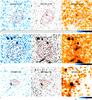 |
Fig. 1 HST ACS B band (left panel), z band (central panel) and HST WFC3 H band (right panel) images of three Chandra-GOODS-ERS sources with overlaid X-ray contours in the 0.7–2.7 keV band (E2199), 0.7–1.9 keV band (E2551) and 0.4–1.5 keV band (E4956). |
Five Chandra-GOODS-ERS sources are present in the 2 Ms direct detection list of Luo et al. , Luo08 hereafter, search within a circle of 1 arcsec radius. Three of them have zphot in Luo et al. , Luo10 hereafter consistent with those in the GOODS-ERS catalog, while in one case the Luo10 zphot is just below 3. One Chandra-GOODS-ERS source is confused/blended in the Luo08 catalog. Eight Chandra-GOODS-ERS sources are present in the 4 Ms direct detection list of Xue et al. , Xue11 hereafter. Two of the three Xue11 sources not in the Luo08 catalog have a photometric redshift, and this is > 3 in both cases. Sixteen Chandra-GOODS-MUSIC sources are present in the Luo08 list, 13 with photometric or spectroscopic redshift consistent with those in the GOODS-MUSIC catalog. Three additional sources are present in the Xue11 catalog, two which have a photometric redshift, and this is consistent with that in the GOODS-MUSIC catalog. Source M 208 was not detected by Luo08, but was detected by Xue11. It is extensively discussed in Gilli et al. .
The accuracy of the photometric redshifts has been greatly improved by the near infrared bands covered by WFC3 (see Tables 1 and 2). The WFC3 coverage also increases the high-z candidate galaxy X-ray detection rate. The ERS area is smaller than one third of the full GOODS area, and therefore, based on the Chandra-GOODS-ERS detections, one would expect ≳ 54 detections in GOODS-MUSIC, while only 41 have been found. Only half of the Chandra-GOODS-ERS detections have a counterpart in the GOODS-MUSIC catalog. We found that 31% and 40% of the Chandra-GOODS-MUSIC detections are also present in the Luo08 2 Ms and Xue11 catalogs. In addition, 28% and 47% of the Chandra-GOODS-ERS detections are present in the same catalogs. We study in more detail the different Chandra-GOODS-MUSIC and Chandra-GOODS-ERS selection effects in Sect. 3.3.
3.1. X-ray and optical spectroscopy
We now discuss the X-ray and optical spectroscopy of our X-ray sources. Unfortunately, only one of the 17 sources in the Chandra-GOODS-ERS sample has optical spectroscopy available. On the other hand, 11 of the 41 sources of the Chandra-GOODS-MUSIC sample have optical spectroscopy available. To exploit this rather large dataset, we complement the full Chandra-GOODS-ERS sample, with the Chandra-GOODS-MUSIC sources that have optical spectroscopy1.
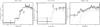 |
Fig. 2 The Chandra X-ray spectra of E537 (Left panel), E1577 (central panel), and M 4835 (right panel). |
We extracted X-ray spectra from the merged event file using source extraction regions of 2–6 arcsec radius, depending on the source off-axis (the Chandra point spread function, PSF, degrades quickly with the off-axis angle). Background spectra were extracted from nearby source-free regions. We also used the total background spectra at three off-axis angles (see the Appendix for details). Background spectra are then normalized to the source extraction region area. We report in Table 3 the results of fitting a simple power-law model to the data. Several Chandra-GOODS-ERS and Chandra-GOODS-MUSIC sources have flat X-ray spectra, which provide strong evidence of large absorbing column densities along these lines of sight. The quality of the spectra is low, but in several cases the statistics are of high enough quality to perform a proper fit with a model including an absorbed power-law or a reflection spectrum. In the following, we briefly outline the main results of this analysis.
-
The source E537 has an extremely hard spectrum. A simple power-law fit produces a negative slope of Γ ~ − 0.15. An absorbed power-law model with Γ fixed to 1.8 yields a column density of NH = 1.6 × 1024 cm-2. A more accurate description of the spectral shape of the low energy spectrum is obtained by adding an unabsorbed power-law (see Fig. 2). The addition of this component provides an excellent fit to the X-ray spectrum of many well-studied obscured AGN. The component appears to be emission produced by the reprocessing of the nuclear continuum by surrounding material and/or a portion of primary radiation leaking through the absorber (see e.g. Turner et al. ; Piconcelli et al. ). The photon index of the soft X-ray component is fixed to Γ = 1.8, while the resulting ratio of the normalization of the unabsorbed to the absorbed power-law is ~ 0.02. An alternative model consisting of a Compton reflection emission component (pexrav model in XSPEC) obscured by a column density of NH = 5 ± 2 × 1023 cm-2 is statistically equivalent.
-
The X-ray spectrum of M 4835 reveals additional complexity when fitted with a simple absorbed (NH = 9 ± 2 × 1023 cm-2) power-law model (C-stat/d.o.f. = 425/442). The best-fit model to the Chandra data includes an additional component produced by X-ray reflection from cold circumnuclear matter. In this case, the primary continuum is obscured by a column density of
 cm-2 and the normalization of the nuclear component is about five times larger than that of the reflection component. Finally, the limit equivalent width (EW) of the Fe Kα emission line measured with respect to the reflection continuum is < 1.1 keV, i.e. still consistent with the expectation of a reflection model. Figure 2 shows the Chandra spectrum of M 4835 fitted by this reflection + transmission model.
 -
The source M 5390 is G202, the well-known, highly obscured QSO discovered by Norman et al. at z = 3.7. The Chandra spectrum is consistent with the XMM one presented by Comastri et al. . It is well-fitted by a power-law model (with Γ = 1.8 fix) absorbed by a column density of NH ~ 1.2 ± 0.15 × 1024 cm-2 and Gaussian line (E = 6.6 keV, likely a blend of the 6.4 keV neutral Fe and 6.7 keV Fe XXV Kα lines, EW = 0.8 ± 0.4 keV), plus an energetically unimportant soft component. The quality of the fit decreases if the continuum is modeled with a pure reflection component.
-
The source M 208 was presented and discussed by Gilli et al. , and we confirm the results reported in that paper, finding the spectrum consistent with being obscured by a Compton thick absorber. Very similar results are obtained for E1577, which is best fitted by a heavily absorbed (i.e. NH ≥ 1024 cm-2) power-law model (see Fig. 2). We also detected obscuration with column density values consistent with 1024 cm-2 in the spectrum of E8479.
-
Large NH values exceeding 1023 cm-2 (but still in the Compton-thin regime) are reported from the spectral analysis of E1617, M 8273, M 4302, and M 3320. Remarkably, in the spectrum of the latter source at z = 3.471, we found clear evidence of an emission line with an EW = 160 ± 100 eV at a best-fit rest-frame energy of 6.97 keV and, therefore, associated with highly ionized (i.e. Fe XXVI) iron.
In conclusion, at least 3 of the 17 Chandra-GOODS-ERS sources are likely to be Compton thick AGN, that is  of the AGN in the sample are Compton thick, as well as 4 of the 11 Chandra-GOODS-MUSIC AGN with spectroscopic redshift (one of these sources is in common with the Chandra-GOODS-ERS sample). An additiona three Chandra-GOODS-MUSIC and one Chandra-GOODS-ERS AGN are highly obscured. The luminosity of the Compton thick ERS and GOODS-MUSIC AGN is in the range log (L2–10 keV) = 43.5–44.5, i.e. between bright Seyfert 2 galaxies and type 2 QSOs. The 2–10 keV flux of the Chandra-GOODS-ERS sources is between 0.3 and 3 × 10-16 erg/cm2/s. At these fluxes, the Gilli et al. model for the cosmic X-ray background (CXB) predicts a fraction of Compton thick AGN of ~ 20%. This is similar to the fraction of Compton thick AGN that we find at z > 3, thus suggesting that Compton thick AGN are probably more common at high-z than previously predicted (also see Gilli et al. ).
It is instructive to compare the result of the X-ray spectroscopy to those of the optical spectroscopy, photometry, and morphology in Table 3. The two CT AGN for which CIV is redshifted in the band covered by optical spectroscopy have narrow CIV lines, in addition to narrow Lyα lines. One of these (E1577/M 13549) also displays broad absorption blueward of CIV. The highest redshift CT AGN (M 208) has a narrow Lyα and a relatively broad (2000 km s-1) NV emission line (also see Gilli et al. ). Two of the three highly obscured AGN (M 3320 and M 8273) also have narrow Lyα emission lines and, when redshifted to the band covered by the spectroscopy, narrow CIV lines. In the spectrum of the third highly obscured source (M 4302), strong and broad absorption lines are present.
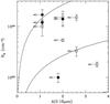 |
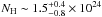
Fig. 3 The best-fit NH as a function of the 0.16 μm extinction for the 10 z > 3 highly obscured or Compton thick AGN. Filled points are sources with point-like optical or near infrared morphology. The two solid lines are the expectation for a dust-to-gas ratio 100 and 1000 times lower than the Galactic one. |
Multiwavelength properties of z > 3 galaxies.
Four of the ten highly obscured and Compton thick AGN have a point-like morphology in the z band (M 13549/E1577, M 5390, M 4302, M 208) or H band (E1577) based on the class_star parameter of sextractor, FWHM measurements, and eye-ball inspection of z and H band images. This suggests that the active nucleus contributes significantly to the UV and optical rest-frame emission, as confirmed in M 4302 and M 13549/E1577 by the detection of likely nuclear broad absorption lines in their UV rest-frame spectra.
We estimated the rest-frame UV (0.16 μm) extinction of the highly obscured and Compton thick AGN by fitting their observed spectral energy distribution (SED) with galaxy templates and the Calzetti et al. extinction law. Table 3 gives the 1σ upper limit to A(0.16 μm), along with the A(0.16 μm) lower limit obtained using the 1σ lower limit to the neutral gas absorption column density and assuming a Galactic dust-to-gas ratio. We also plot for these sources the best-fit NH and A(0.16 μm) upper limits in Fig. 3. We see that NH measurements and the A(0.16 μm) limits of all ten highly obscured or Compton thick AGN are completely inconsistent with a Galactic dust-to-gas ratio. This is also true for the four objects with point-like morphology. The same conclusion is reached by estimating dust extinction from the galaxy stellar masses. It is difficult to estimate accurate stellar masses for our high-z AGN, but they likely exceed several 1010 M⊙. The extinction expected based on the correlations found by Pannella et al. in a sample of z ~ 2 BzK galaxies is of 3–6 mag at 1500 Å. We conclude that, at least for the four point-like objects, the dust-to-gas ratio of the absorbing matter is likely 1/100–1/1000 that of the Galaxy. This is also lower than in the (mostly low-z) AGN studied by Maiolino et al. and Shi et al. . The low dust-to-gas ratio can be explained if the absorbing matter is within of close to the dust sublimation radius. The other six highly obscured or Compton thick AGN have extended morphologies in the z and H images, suggesting that young stellar populations contribute significantly to the UV and optical rest-frame emission. In these cases, little can be said about either the nuclear extinction and the dust-to-gas ratio.
3.2. Radio counterparts and star-formation rates
Two Chandra-GOODS-ERS sources (E2551 and E1611/ M 70107) and another five Chandra-GOODS-MUSIC sources (M 2690, M 4835, M 8273, M 70091, and M 70340) have a detection at 1.4 GHz in the DR2 catalog of the VLA-CDFS survey Miller et al. . Radio fluxes for the Chandra-GOODS-ERS sources and the Chandra-GOODS-MUSIC sources with spectroscopic redshift are given in Table 3. Anther 8 sources in Table 3 have a faint radio signal at the position of the galaxy (signal-to-noise ratio of between 2.4 and 3.2). The probability of this signal consisting of background fluctuations is < 2%, corresponding to < 1 spurious radio detection in the full sample of sources in Table 3. We also report in Table 3 radio fluxes for the additional 8 faint detections. We stress that the latter faint fluxes may over-estimate the real radio flux because of the Eddington bias. A more robust average flux can be obtained by stacking together the radio images at the position of the X-ray sources. The average flux for the Chandra-GOODS-ERS and Chandra-GOODS-MUSIC sources without a detection in the DR2 VLA-CDFS catalog is 6.5 ± 1.5 μJy and 10.1 ± 1.1 μJy, respectively.
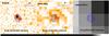 |
Fig. 4 K band, MIPS 24 μm, and LABOCA 870 μm images around the M 4417 galaxy with overlaid X-ray 0.5–3.2 keV contours. |
The observed radio fluxes can be produced by both nuclear and stellar processes. Using the La Franca et al. probability distributions for the X-ray to radio nuclear luminosity, we expect a L(2–10 keV)/L(1.4 GHz) ratio < 3 × 10⁴ for ~ 25% of the sources in Table 3, and L(2–10 keV)/L(1.4 GHz) < 103 for 5% of the sources. We converted the radio fluxes in Table 3 into luminosities using the expression  (1)where DL is the luminosity distance in Mpc and f(1.4 GHz) is in μJy and we assumed α = 0.7. We found in all cases that L(2–10 keV)/L(1.4 GHz) < 3 × 10⁴, which is 41% of the full sample, and L(2–10 keV)/L(1.4 GHz) < 103 for 5 sources, i.e. 18% of the full sample. This difference between the expected and observed fraction of radio bright sources is not conclusive, because our radio fluxes may be over-estimated as discussed above. However, if we associate to the sources without a detection in the DR2 VLA-CDFS catalog the average flux measured above, the fractions of sources with L(2–10 keV)/L(1.4 GHz) < 3 × 10⁴ and L(2–10 keV)/L(1.4 GHz) < 103 are 92% and 19%, respectively. We can therefore conclude that, at least on average, radio fluxes are higher than expected based on the X-ray fluxes and assuming a common nuclear origin. If radio emission is dominated by stellar processes (as also suggested by Padovani et al. ), we can convert radio fluxes into star-formation rates (SFRs, see e.g. Yun et al. ). We used the a calibration that assumes a Chabrier IMF2
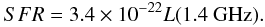 (2)In two cases, we have independent estimates of SFR, which agree reasonably well with the values in Table 3. We find that M 208, has a SFR ~ 1000 M⊙/yr, as estimated from a Laboca 870 μm detection (see Gilli et al. ), while M 4417 has SFR ~ 440 M⊙/yr, as estimated from UV SED fitting and oxygen lines (Maiolino et al. ).
3.2.1. A high-z star-forming galaxy?
A rather peculiar case is M 4417, a galaxy studied by Maiolino et al. in the framework of the AMAZE program. The X-ray luminosity corresponding to the observed SFR is log L(2–10 keV) ~ 42.35 (by using the Ranalli et al. conversion factor), just a factor 40% lower than the observed X-ray luminosity. We note that although the Chandra X-ray contours seems to be centered on M 4417 (see Fig. 4), there could be some contribution to the observed X-ray flux from the nearby z = 3.471 galaxy M 4414, which has a SFR that is about a quarter of that of M 4417. Intriguingly, M 4417 is the Chandra-GOODS-MUSIC and Chandra-GOODS-ERS object with the lowest X-ray to z band and H band flux ratios (0.004 and 0.005 respectively), which is lower than for typical AGN (see next section), and implies that the X-ray emission from this object is not dominated by a nuclear source. We then conclude that the observed X-ray luminosity is likely dominated by stellar sources, making M 4417 one of the farthest objects in which X-rays permit us to investigate stellar processes. Alternative solutions are of course possible, for example M 4417 may be a reflection-dominated, heavily Compton thick AGN, where the nucleus is completely hidden and the observed X-ray luminosity is just a fraction of the real one. However, we are unable to justify this interpretation using either X-ray colors, optical spectroscopy, infrared spectroscopy, or broad-band UV to infrared SED (the source is not detected at wavelengths longer than 8 μm, see Fig. 4).
There are another two sources with relatively low X-ray luminosity and high radio flux: E2551 and E1516. In these cases, the X-ray luminosity corresponding to the SFR rate estimated from the radio flux is a factor of 70% and 90% lower than the observed X-ray luminosity. Their X-ray to H band ratio are however ≳ 10 times higher than that of M 4417 (0.06 for E2551 and 0.07 for E1516). The radio flux and luminosity of E2551 are the highest in the sample, suggesting that it may well be a radio loud AGN.
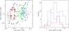 |
Fig. 5 Left panel: the X-ray to NIR flux ratio F(0.5–2 keV)/F(H) as a function of the X-ray flux for the z > 3 Chandra-GOODS-ERS AGN sample (red-filled circles), Chandra-GOODS-MUSIC sample (black-open circles), Chandra-COSMOS sample (green-filled squares) and XMM-COSMOS sample (blue-filled triangles. Right panel: the distributions of F(0.5–2 keV)/F(H) for the Chandra-COSMOS z > 3 sample (black histogram), Chandra-ERSVO sample (red histogram), and Chandra-GOODS-MUSIC sample (blue, dashed histogram). |
Chandra-GOODS-ERS z > 3 AGN comoving space densities.
3.3. X-ray to optical/NIR flux ratios and selection effects
The standard procedure for assembling X-ray high-z AGN samples is based on the optical identification of X-ray source catalogs. In the previous section, we used a complementary approach, which involves studying the X-ray emission of either optically or NIR selected high-z galaxies. In the first case, the problem is to be sure that the optical/NIR identification of the X-ray source is correct, and that sample identifications are reasonably complete. In the latter case the problem is the reliability and completeness of the optical/NIR samples. They should include most of the galaxies (and therefore most AGN) down to a reasonably low flux limit. The GOODS-MUSIC catalog is fairly complete down to z ~ 26 and F(4.5 μm) ~ 1.5 μJy and includes sources down to z ~ 27 and F(4.5 μm) ~ 0.5 μJy. The GOODS-ERS catalog is fairly complete down to H ~ 26.5 and includes sources down to H ~ 27.5. To understand how these optical and NIR flux limits translate into X-ray flux limits, we compute the X-ray (0.5–2 keV) to NIR (H band) flux ratio F(0.5–2 keV)/F(H) of much brighter, and therefore likely complete, AGN samples. Figure 5 compares F(0.5–2 keV)/F(H) of the z > 3 Chandra-GOODS-ERS and Chandra-GOODS-MUSIC AGN samples to the Chandra-COSMOS (Civano et al. ) and XMM-COSMOS (Brusa et al. ; ) z > 3 AGN samples. The COSMOS samples are X-ray selected samples with nearly complete optical identification, because they cover X-ray and optical/NIR fluxes that are 10–100 times brighter than the Chandra-GOODS-ERS and Chandra-GOODS-MUSIC AGN samples, and thanks to the massive photometric campaigns performed in this field with HST/ACS, Subaru, and CFHT (Capak et al. 2008). As an example, there are only two sources in the Chandra-COSMOS catalog without either an optical or infrared counterpart, 19 without an optical counterpart, 0.1% and 1% of all Chandra-COSMOS sources respectively, Civano et al. . Most of these sources are likely high-luminosity, highly obscured type 2 QSOs (e.g. Fiore et al. ). However, even assuming that all these 19 sources are at high-z, they would be 25% of the z > 3 sources in Chandra-COSMOS. Hence this is a very conservative upper limit to the Chandra-COSMOS completeness at high-z. Similar numbers apply to the XMM-COSMOS survey.
The Chandra-GOODS-ERS detections cover a range of F(0.5–2 keV)/F(H) values that are similar to the COSMOS samples and indeed the Chandra-GOODS-ERS and COSMOS distributions of F(0.5–2 keV)/F(H) are perfectly consistent: the probability that the Chandra-GOODS-ERS and Chandra-COSMOS distributions are drawn from the same parent population is indeed 50%, using the Kolmogorov-Smirnov test. This suggests that the HST/WFC3 ERS H band images are deep enough to trace high-z AGN populations at the extremely faint X-ray flux limits reached by the Chandra 4 Ms exposure, avoiding significant incompleteness, or at least with an incompleteness comparable to that reached at much brighter fluxes by Chandra-COSMOS and XMM-COSMOS. The same exercise performed using the GOODS-MUSIC z band and IRAC 4.5 μm selected catalog was unsuccessful: we used a subsample of the full Chandra-GOODS-MUSIC sample with deep H band VLT/ISAAC coverage, excluding 13 sources with shallower H band coverage. The Chandra-GOODS-MUSIC sample clearly misses sources with high F(0.5–2 keV)/F(H) flux ratio in comparison to the Chandra-GOODS-ERS and COSMOS samples, and indeed the Chandra-GOODS-MUSIC F(0.5–2 keV)/F(H) distribution is inconsistent with the Chandra-COSMOS distribution at the 99.925% confidence level (using the Kolmogorov-Smirnov test). This means that the GOODS ACS and IRAC images are insufficiently deep to fully probe the AGN population at the flux limits of the CDFS 4 Ms observation. The F(0.5–2 keV)/F(H) distribution of the Chandra-GOODS-MUSIC sources with F(0.5–2 keV) ≳ 5 × 10-17 erg/cm2/s is consistent with the GOODS-ERS and COSMOS ones (probability of ~30% that they can be drawn from the same parent population), hence in the following we consider only the 23 Chandra-GOODS-MUSIC sources brighter than this flux limit (and outside the ERS area). These 23 sources are added to the 17 sources of Chandra-GOODS-ERS sample to form a total sample of 40 high-z AGN. We use this sample to constrain the faint end of the AGN luminosity function at high redshift.
4. High-z AGN luminosity functions
Our z > 3 AGN candidate sample includes 17 Chandra-GOODS-ERS sources and 23 Chandra-GOODS-MUSIC sources spanning a range in luminosity of 42.5 < log L(2–10 keV)/erg/s < 44.8. They can be used to probe the faint end of the high-z AGN luminosity functions. We calculated the comoving space densities of our high-z sample using the 1/Vmax method (Schmidt ). We chose L(2–10 keV) and z ranges to ensure completeness at the X-ray flux limit F(0.5–2 keV) ~ 2 × 10-17 erg/cm2/s reached by our survey. The luminosity limit at z = 4, 5, and 7.5 is log L(2–10 keV) ~ 42.7, 42.8, and 43.3, respectively. Accordingly, we computed comoving space densities in the redshift bins 3–4, 4–5, and 5.8–7.5, with luminosity ranges 42.75–44.5, 43–44, and 43.5–44.5, respectively. There are a total of 30 Chandra-GOODS-ERS and Chandra-GOODS-MUSIC AGN in these redshift and luminosity bins. Comoving space densities are given in Table 4. Figure 7 presents the AGN luminosity functions in the same redshift bins. Errors are computed by evaluating the Poisson statistics for the number of AGN in each redshift-luminosity bin. To obtain information about the slope of the luminosity functions, we joined the above samples to the Chandra-COSMOS high-z sample of Civano et al. , the XMM-COSMOS sample of Brusa et al. , the GOODS sample of Fontanot et al. , the faint optical AGN sample of Glikman et al. , and the luminous optical AGN samples of Richards et al. and Jiang et al. . We converted the rest-frame 1450 Å luminosities of the optically selected samples to the 2–10 keV band using the Marconi et al. and Sirigu et al. 2011 luminosity-dependent conversion factors. We assumed no intrinsic reddening in the optically selected high-z AGN. This might underestimate the real AGN luminosity, if significant dust is present along the high-z AGN lines of sight (Maiolino et al. ; Jiang et al. ; Gallerani et al. ). We checked our conversion factors using real data, that is the Chandra and XMM detections of the Jiang et al. QSOs (Mathur et al. ; Shemmer et al. , and references therein). Figure 6 shows the ratio of the UV 1450 Å luminosity to the 2–10 keV luminosity against 1450 Å luminosity for 12 QSOs at z > 5.7, for which we collected X-ray data from the literature. The figure also shows the UV to X-ray conversion adopted in this work, which agrees quite well with the data of this high-redshift QSO sample.
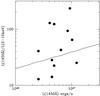 |
Fig. 6 The UV 1450 Å to X-ray 2–10 keV luminosity ratio for 12 QSOs at z > 5.7. |
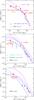 |
Fig. 7 The AGN 2–10 keV luminosity functions at z = 3–4 (top panel), z = 4–5 (central panel), and z > 5.8 (bottom panel). Large red-filled circles are from the CDFS Chandra-GOODS-MUSIC and Chandra-GOODS-ERS samples. Red-filled triangles are from Chandra-COSMOS (Civano et al. 2011), red-filled squares from XMM-COSMOS (Brusa et al. 2010). The blue thick curve in the top panel is the LADE model of Aird et al. (2010) in the 2.5–3.5 redshift bin. Large black-open triangles are SDSS data from Richards et al. (2006), stars are SDSS data from Jiang et al. (2009), open circles are from Glikman et al. (2011), and small blue-open triangles are from Fontanot et al. (2007). Black dashed curves are best fits to the X-ray plus optical, wide-luminosity-range luminosity functions (see text for details). Magenta solid curves encompass the predictions of the Menci et al. (2006, 2008) semi-analytic model. Blue curves are models from Shankar et al. (2011, see the Discussion for details). |
Modeling the high redshift AGN luminosity function.
We modeled the wide luminosity range high-redshift luminosity functions using the standard double power-law shape ![Mathematical equation: \begin{equation} \frac{{\rm d} \Phi (L_{\rm X})}{{\rm d log} L_{\rm X}} = A \left[(L_{\rm X}/L_{*})^{\gamma 1} + (L_{\rm X}/L_{*})^{\gamma 2}\right]^{-1}, \end{equation}](/articles/aa/full_html/2012/01/aa17581-11/aa17581-11-eq191.png) (3)where A is the normalization factor for the AGN density, γ1 and γ2 are the faint-end and bright-end slopes, and L ∗ is the characteristic break luminosity. Optical selection may miss highly obscured AGN, which can represent a large fraction of the total in particular at low luminosity (La Franca et al. ). To avoid possible incompleteness in optical surveys, we excluded from the fit the optically selected AGN density determinations with M1450 > − 26.5 (or correspondingly L(2–10 keV) < 45.1). We first fitted this simple model to the luminosity functions in the three redshift bins. The number of points in the z = 3–4 redshift bin allows us to constrain all four parameters. This is impossible in the redshift bins 4–5 and > 5.8, where we fitted the data fixing the slopes γ1 and γ2 to the best-fit values found in the z = 3–4 redshift bin. The results of these fits are reported in Table 5. As a next step, we fitted simultaneously the data in the three redshift bins with an evolutionary model. We chose to describe the evolution of the high-z AGN luminosity function with the LADE (luminosity and density evolution) model, introduced by Aird et al. . Thus, the evolution of L ∗ is given by
(3)where A is the normalization factor for the AGN density, γ1 and γ2 are the faint-end and bright-end slopes, and L ∗ is the characteristic break luminosity. Optical selection may miss highly obscured AGN, which can represent a large fraction of the total in particular at low luminosity (La Franca et al. ). To avoid possible incompleteness in optical surveys, we excluded from the fit the optically selected AGN density determinations with M1450 > − 26.5 (or correspondingly L(2–10 keV) < 45.1). We first fitted this simple model to the luminosity functions in the three redshift bins. The number of points in the z = 3–4 redshift bin allows us to constrain all four parameters. This is impossible in the redshift bins 4–5 and > 5.8, where we fitted the data fixing the slopes γ1 and γ2 to the best-fit values found in the z = 3–4 redshift bin. The results of these fits are reported in Table 5. As a next step, we fitted simultaneously the data in the three redshift bins with an evolutionary model. We chose to describe the evolution of the high-z AGN luminosity function with the LADE (luminosity and density evolution) model, introduced by Aird et al. . Thus, the evolution of L ∗ is given by  (4)and the evolution of A is given by
  (5)We first fitted the data with the full six-parameter model. The γ1 and γ2 slopes were found to be similar to those obtained fitting the z = 3–4 data only (the z = 3–4 data provides the strongest constraint on the shape of the luminosity function). We report in Table 5 the best-fit parameters obtained by fixing γ2 to 3.4 and 3.0 (keeping the faint-end slope γ1 fixed in both cases at 0.8). The fit with γ2 = 3 produces a χ2 value that is larger than for the best-fit case, but still acceptable considering the uncertainties in the correction between the optical and X-ray luminosities for the optically selected AGN density determinations. We found that the A0 and d parameters are completely degenerate. We could obtain equally good fits for combinations of A0 and d that were inversely correlated. We report in Table 5 the best fits obtained with d = 0 (no density evolution) and d = −1. The data are good enough to constrain relatively well L0 and p. Our data are thus consistent with a pure luminosity evolution, with L ∗ rather quickly reducing with redshift. The dashed lines in Fig. 7 are the best-fit pure-luminosity evolution model (4) in Table 5.
It is not straightforward to compare our high-z, wide-luminosity-band luminosity functions with previous determinations. The best-fit model of Shankar et al. agrees quite well with our determinations at log L(2 − 10 keV) < 44 but overestimate the density of higher luminosity AGN, in particular of optically selected AGN. We note that Shankar et al. adopt a UV to X-ray luminosity conversion factor fixed at 10.4, while our conversion factor varies with luminosity, from 4.4 at log L(2–10 keV) = 43 to 27 at log L(2–10 keV) = 45. Furthermore, Shankar et al. correct for extinction and the fraction of Compton thick AGN. As discussed above, our data are not corrected for the fraction of Compton thick objects, because several have been found in our samples, and we used optically selected AGN of high luminosity (M1450 > −26.5, L(2–10 keV) < 45.1), where the fraction of obscured AGN is likely to be small. Hopkins et al. use a luminosity-dependent bolometric correction, but with a different calibration from ours. They correct their data for extinction and the fraction of Compton thick AGN missed in optical, X-ray, and infrared surveys. They convert NH distributions evaluated from X-ray data into optical-UV reddening using a canonical gas-to-dust ratio, which, as discussed in the previous section (and by e.g. Maiolino et al. ; Shi et al. ), can overestimate the real extinction, in particular when the X-ray absorber is compact, smaller than the dust sublimation radius. They find z > 3 luminosity functions with much flatter slopes than ours (or to the Shankar et al. , ones). As an example, the Hopkins et al. best-fit model would predict ~2−4 times more z = 3–4 and z = 4–5 AGN with log L(2–10 keV) > 44.5 than actually found in the XMM and Chandra COSMOS surveys (Brusa et al. ; Civano et al. ).
4.1. AGN luminosity function and duty cycle evolution
We now place our findings in Sect. 4 in a context that enables us to study the evolution of the AGN luminosity function from the local Universe to z ~ 6. We compare in the upper panel of Fig. 8 the best fits to both the z = 3.5, z = 4.5, and z = 6 AGN luminosity functions (model 4 in Table 5) and the best-fit model luminosity functions found at lower redshift by La Franca et al. . These were computed by correcting for the incompleteness caused by X-ray absorption, which is significant at low redshift where the photoelectric cut-off produced by the typical column densities observed in many AGN is well within the X-ray selection band. The La Franca et al. luminosity functions are consistent with the more recent determinations of Aird et al. and Ebrero et al. , which are both based on a larger number of objects. The upper panel of Fig. 8 summarizes the complex evolution of the AGN luminosity function, which increases between z = 0 and z = 1, 2, and 3 for increasing luminosities and then decreases at yet higher redshifts.
We converted these luminosity functions into “active” SMBH mass functions using Monte Carlo realizations. We simulated 108 AGN luminosities and SMBH masses in each redshift bin according to the following procedure. We first randomly chose an X-ray luminosity following the luminosity function distribution in each given redshift bin. We then converted it into a bolometric luminosity using the Marconi et al. and Sirigu et al. (2011) luminosity-dependent bolometric correction. Next, we randomly chose an Eddington ratio from log-normal distributions with parameters given in Table 6. At z < 0.3, we used the distribution of Netzer , which are shifted toward higher Eddington ratios with respect to the Kauffmann & Heckman distributions (see the discussion in Netzer ; ). At medium to high redshift, we used the distributions of Trakhtenbrot et al. , Shemmer et al. , Netzer & Trakhtenbrot , and Willott et al. . This provides a SMBH mass for each chosen X-ray luminosity and Eddington ratio. We finally binned the resulting SMBH distributions in each redshift bin to build SMBH mass functions. The resulting “active” SMBH mass functions in six redshift bins are plotted in the central panel of Fig. 8. It must be stressed that this is an empirical calculation, performed independently for each redshift bins, using only observed quantities. It does not pretend to model the history of SMBH growth during the cosmic time, which can be obtained using a continuity equation and conserving the number, as in Marconi et al. ; Merloni & Heinz ; Shankar et al. .
Furthermore, the adopted Eddington ratio distributions all refer to relatively luminous AGN. Less active SMBH, which relate to low luminosity AGN and LINERs, are not represented in these distributions. For this reason, we adopted a luminosity limit for the computed SMBH mass functions: these functions represent “active” SMBH producing an X-ray luminosity > 1043 erg/s. As a consequence, any comparison with previous calculation is not straightforward. For example, while our SMBH mass functions are luminosity limited, the “active” SMBH mass functions of Merloni & Heinz are X-ray flux-limited mass functions. The 2–10 keV luminosity corresponding to the faintest flux limit of Merloni & Heinz is ~1040 erg/s at z = 0.1, and ~1043.5 erg/s at z = 3, while we plot the SMBH mass function of AGN that are more luminous than ~1043 erg/s in all redshift bins. The SMBH mass functions of broad-line AGN have been computed by Kelly et al. (2010) using about 10 000 SDSS QSOs in the redshift range 1–4.5. Our SMBH mass functions are consistent, or slightly higher than the Kelly et al. determinations at most redshifts and black hole masses considered, as expected since broad lines AGN are a fraction of the full active SMBH population, even at the highest SMBH masses and/or AGN luminosities. The only regime where our estimates are significantly higher than the Kelly et al. ones is that of the highest masses (log M > 9.3 M⊙) at z ~ 1, where the Kelly et al. (2010) function drops steeply, while our function decreases more smoothly.
The SMBH mass functions can be transformed into stellar mass functions of “active” galaxies by assuming a conversion factor between SMBH mass and host galaxy stellar mass. We assumed a mean value Γ0 = log (MBH/M ∗ ) = −2.8 at z ~ 0 (Haring & Rix but also see the discussion in Lamastra et al. ) and a redshift evolution Γ ~ Γ0 × (1 + z)0.5 (Merloni et al. ; Hopkins et al. ; Shankar ). We note that in the local Universe the above correlation has been found and calibrated for the bulge component of galaxies. Whether a strict distinction between bulge and disk also exists at high-z is a matter of debate. Disks of z ~ 2 galaxies are much more compact and much thicker that in today spirals of similar mass (Genzel et al. ; van der Wel et al. ). For the sake of simplicity, we assume in the following calculation that the SMBH mass is proportional to half of the total stellar mass of high-z galaxies. It is instructive to compare the SMBH mass functions and the “active” galaxy stellar mass functions to the stellar mass functions of all galaxies. The lower panel of Fig. 8 plots a collection of galaxy stellar mass functions: we used the stellar mass functions of Fontana et al. at z ≲ 2, Santini et al. at z = 3–4, Caputi et al. at z = 4–5, and Stark et al. at z = 6.
Parameters of log-normal Eddington ratio distributions.
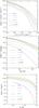 |
Fig. 8 Top panel: a collection of AGN luminosity functions at z ≲ 2 from La Franca et al. (2005), and z > 3 in this work. Central panel: SMBH mass functions obtained by combining the AGN luminosity functions in the top panel with Eddington ratio distributions (see the text for details). Bottom panel: a collection of galaxy stellar mass functions. z ≲ 2 from Fontana et al. (2006), z = 3–4 from Santini et al. (2011), z = 4–5 from Caputi et al. (2011), and z = 6 from Stark et al. (2009). |
The AGN fraction, or AGN duty cycle, can finally be obtained by dividing the “active” galaxy stellar mass functions by the galaxy stellar mass functions. Following the adopted luminosity limit used to compute SMBH mass functions, we define the AGN duty cycle as the fraction of AGN with 2–10 keV luminosity greater than 1043 erg/s to the total number of galaxies with a given stellar mass. Lower luminosity AGN do exist and are probed by the luminosity functions in Fig. 8 up to z ~ 2−3. However, they are below the flux limit of current surveys at higher redshift. Therefore, our luminosity threshold also avoids problems caused by the incompleteness of the samples at high-z. According to this definition, the AGN duty cycle can differ from the AGN timescale, since the latter is correlated with the total intrinsic lifetime of the AGN, which can include phases of luminosity <1043 erg/s. The AGN duty cycle is plotted in the upper panel of Fig. 9. It must be stressed again that this is an empirical calculation, performed independently for each redshift bin, using only the observed AGN and galaxy luminosity and mass functions and the observed Eddington ratio distributions. We found that the AGN duty cycle increases at all redshift with the stellar mass. Similar trends have been found by Kauffmann et al. , Best et al. , Bundy et al. , Yamada et al. , and Brusa et al. for optically-selected, radio-selected, and X-ray selected AGN. At each given stellar mass, the duty cycle increases with redshift up to z = 4–5, which is consistent with the results of Marconi et al. ; Brusa et al. , and Shankar et al. . There are 22 galaxies in the GOODS-ERS catalog with z > 3 and stellar mass higher than 1011.25 M⊙, 7 of which are X-ray sources in Table 1, thus confirming an AGN duty cycle ≳ 30% at z > 3 for these massive galaxies. Figure 9, lower panel, plots the evolution of the AGN duty cycle as a function of redshift for two galaxy stellar masses: log(Ms) = 11.25 and 11.75. Bands are plotted rather than curves to emphasize the rather large uncertainties, especially at high-z (see next section). The same figure shows the previous evaluations of Brusa et al. . These are consistent with the present estimates within their rather large error bars. The expectations of the Menci et al. semi-analytic model are also shown in the lower panel of Fig. 9.
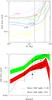 |
Fig. 9 Top panel: the AGN duty cycle as a function of the galaxy stellar mass in six redshift bins. AGN with log L(2–10 keV) > 43 are considered only. Bottom panel: the AGN duty cycle as a function of redshift for two galaxy stellar masses (log M∗ = 11.25, 11.75 M⊙). Filled circles and triangles are the previous determination of Brusa et al. (2009b) for the same masses. The black dashed (dotted) curve is the prediction of the Menci et al. (2006, 2008) SAM for log M∗ = 11.25 M⊙ (log M∗ = 10 M⊙). |
4.1.1. Error budgets
The determination of the evolution of the AGN duty cycle is plagued by large uncertainties, especially at high redshifts. It is therefore important to study in detail the origin of these uncertainties and any way of reducing them.
The uncertainty in both the AGN comoving densities at z < 2 (at least for unobscured and moderately obscured AGN) and in the stellar mass functions at z < 2 are relatively small, of approximately 10–20% or even smaller, thanks to large AGN and galaxy samples used for these determinations and the use of several different surveys, which helps in reducing the systematic error. The largest uncertainty in the AGN luminosity function is in the fraction of Compton thick AGN. The fraction of these objects in the local Universe is high: 30–50% of the optically selected Seyfert 2 galaxies can be Compton thick (≈1/4−1/3 of the full AGN population, Risaliti et al. , Panessa et al. , a result confirmed by hard X-ray selection, see Malizia et al. ). At higher redshift, the fraction of Compton thick AGN is more uncertain, but it can be as high as one third of the full AGN population (Fiore et al. ; ), or even higher (Daddi et al. ; Treister et al. ). A fraction of Compton thick sources about one third of the total is actually included in the model of La Franca et al. , hence we are confident that the error in the total AGN comoving space density at z < 2 caused by undetected, and unaccounted-for, Compton thick sources is small ( ≲ 10 − 20%)
At z > 3, the uncertainties in both AGN luminosity function and galaxy mass functions are larger, in particular at low AGN luminosities and low galaxy masses (see Table 3), they are of the order of 30–50% for z = 3–5. At z ~ 6, the uncertainties in the faint end of the AGN luminosity function and the galaxy stellar mass function are extremely large, a factor of 100%. These uncertainties are dominated by statistics in the case of AGN (only a few detections at z > 4–5) and by systematics in the case of the galaxy mass function (at z ~ 6, stellar masses were estimated by Stark et al. by converting the UV luminosity into stellar mass, which is a highly uncertain procedure). The uncertainty caused by undetected or unaccounted-for Compton thick AGN at z > 3 is smaller than the above features. We note that at z > 3 the cut-off produced by a column density 1024 cm-2 is shifted below 2.5 keV, where the effective area of Chandra and XMM reaches a maximum. This, together with the extremely deep exposures of the CDFS, helps us detect directly at least mildly Compton thick sources (Georgantopoulos et al. ; ; Feruglio et al. ; Gilli et al. ; Comastri et al. ). About one fifth of the Chandra-GOODS-ERS sources might indeed be Compton thick, as well as one fourth of the Chandra-GOODS-MUSIC sources with optical spectroscopy (see Sect. 3.2), and many are directly detected in our z > 3 search. We are therefore confident that the uncertainty in the total AGN comoving density linked to Compton thick AGN is at most ~ 10 − 20% also at z > 3. The high luminosity end of our z > 3 luminosity functions is probed by optical surveys. Obscured AGN may well be missed by these surveys, and therefore these determinations may be regarded as lower limits. We note, however, that the fraction of obscured AGN decreases strongly with the luminosity (at least at z < 2–3 where large area X-ray surveys provided samples of high luminosity QSOs), hence the error in the comoving space density of high luminosity AGN at z > 3 is also likely to be small ( < 20%). We should consider the uncertainty in the conversion from UV to X-ray luminosities for the optically selected AGN luminosity functions. This uncertainty is probably of the order of 30% (see the discussion in Shankar et al. 2009a).
Another relatively large source of error in the evaluation of the AGN duty cycle is the uncertainty in the Eddington ratio distributions. We performed several tests using parameters slightly different from those in Table 6. For these AGN, we found that the duty cycle (at log M∗ = 11) changes by a factor of 15–30% and ~ 100% for distribution peak and width differing by 30% from the assumed ones. The biggest effect is introduced by the width of the Eddington ratio distributions: the broader the distribution, the higher the resulting AGN duty cycle. The uncertainty in the Eddington ratios is particularly severe for low luminosity AGN, with log L(2–10 keV) < 43. Since this is also, roughly, the luminosity limit of our z > 3 sample, we decided to limit the analysis to AGN with logL(2–10 keV) > 43 erg/s only, and assume conservatively a 50% (total) relative error in the AGN duty cycle arising from the uncertainty in the Eddington ratios.
Finally, we adopted both a given normalization and a given evolution of the SMBH to galaxy stellar mass ratio Γ that is identical for each object at each given redshift. However, we know that, at least at low redshift, the SMBH-bulge mass relation is unlikely to be universal (Mathur et al. ; ; Graham et al. , and references therein). Furthermore, Batcheldor suggest that selection effects are important in shaping the SMBH-bulge mass relation. Thus, the deviations in the SMBH mass-bulge mass relations resulting from galaxy morphology, orientation, and selection effects can affect the duty cycle calculations, in particular at low galaxy masses. We assumed a redshift evolution (1 + z)0.5, which is consistent with our present knowledge and with expectation of several models, including those of Lamastra et al. , Hopkins et al. , and Shankar et al. . However, the uncertainty in this calibration increases with redshift, and can be rather large at z > 3–4. Quantifying all these effects is not an easy task. For example, if Γ is half of that assumed above, the duty cycle is reduced by a factor between 20% and 100%, depending on the galaxy stellar mass and redshift. In summary, the bands plotted in Fig. 9 roughly account for the typical errors given above at each given redshift and galaxy stellar mass.
5. Discussion
We have evaluated the comoving space density of the z > 3 faint X-ray sources in three redshift bins: 3–4, 4–5, and > 5.8. The number of AGN in the three redshift bins is small, 19, 9, and 2 respectively, thus we have had to use relatively wide luminosity bins, to keep the statistical error reasonably small. In particular, the comoving space density at z > 5.8 and log L(2–10 keV) = 43.5–44.5 has been computed using only two sources. We stress that in one case a secondary solution of the photometric redshift does exist at z ~ 2, hence our determination is probably an upper limit to the true space density of low luminosity AGN at > 5.8. This confirms that the slope of the faint end of the z > 5.8 AGN luminosity function is significantly flatter than the bright end slope (see e.g. Shankar & Mathur ). We also note that the other claimed z > 7 AGN in the CDFS (L306, M 70437) has a 0.5–2 keV flux below our threshold for Chandra-GOODS-MUSIC sources, and its photometric solution for GOODS-MUSIC is broader than that of Luo et al. , with a lower limit at z = 2.7. This source is therefore not part of the z > 5.8 sample used in Fig. 7. Treister et al. evaluated the integrated AGN emissivity at z ~ 6 by stacking together the CDFS and CDFN X-ray data at the position of the z ~ 6 galaxy candidates of Bouwens et al. . They obtained a luminosity density of 1.6 × 1046 erg/s/deg2 in the 2–10 keV band (but also see Fiore et al. ; Willott ). When we integrate our z ~ 6 best-fit model above log LX = 42 we obtain a total luminosity density of 7.5 × 1038 erg/s/Mpc3 or 5.6 × 1045 erg/s/deg2, a value ~3 times smaller than that reported by Treister et al. , but consistent with the Fiore et al. limit.
Our results place some first constraints on the faint end of the AGN luminosity function (42.75 < log L(2 − 10 keV) < 44.5) at z = 3–7, which are interesting to compare with model predictions. To constrain the shape of the AGN luminosity function, we combined our determinations with those obtained at higher luminosities by shallower X-ray surveys (Chandra-COSMOS, XMM-COSMOS) and optical surveys (SDSS, NOAO DWFS/DLS). We then compared the broad luminosity range luminosity functions with the prediction of the semi-analytic model (SAM) of Menci et al. , and Menci et al. . In this model, baryonic processes are associated with the merging histories of dark matter (DM) haloes. These haloes contain hot gas at the virial temperature, a fraction of which can radiatively cool down and form a disk of radius rd and circular velocity vd. During both mergers and less violent galaxy encounters (Cavaliere & Vittorini ), cold gas can loose its angular momentum and be accreted by the nucleus. A fraction of this gas fuels a nuclear starburst, while the rest can be accreted to a central SMBH, giving rise to an AGN. The AGN timescale is τ ≈ rd/vd, i.e. the crossing time for the destabilized gas. Assuming typical values of rd ≈ a few kpc and vd ≈ 100 km s-1, the AGN timescale is short, at a few 107 yr, which is comparable to the Salpeter timescale. In this SAM, the AGN timescale, as well as both the AGN SMBH masses and Eddington ratios, are not free parameters, but are calculated self-consistently (the model only assumes that the accretion can proceed at most at the Eddington limit). The SAM includes a rather detailed treatment of AGN “quasar mode” feedback (Menci et al. ), in terms of a blast wave carrying the AGN power outwards (Lapi et al. ). The SAM predicts the comuving densities of all AGN, which are either unobscured, moderately obscured, or Compton thick. Lamastra et al. compares the SMBH masses and stellar masses of AGN host galaxies predicted by this SAM with measurements for various galaxy and AGN samples at different redshifts. This SAM reproduced reasonably well the z = 3–4 luminosity function at log L(2–10 keV) > 43.5. At lower luminosities, it predicts 2–3 times more AGN than observed. However, some extreme Compton thick AGN, in which the nuclear emission is completely blocked by photoelectric absorption and Compton scattering, leaving only reflection emission in the X-ray band, can be missed even by the deepest X-ray surveys. The agreement is sufficiently good at high luminosities (log L(2−10 keV) > 45) at both z = 4–5 and z > 5.8. In these redshift bins, the agreement between data and model is poorer at lower luminosities, where the Menci et al. SAM predicts 5–10 times more low luminosity AGN than in our determination and 2–3 times more than Treister et al. .
To investigate the origin of this behaviour and gain insights into high-z AGN physics, we compared our measurements with predictions derived from more basic models for AGN activation through galaxy interactions. This class of models consists of two ingredients: a DM halo merger rate compatible with cosmological simulations, and an input AGN light curve (e.g., Wyithe & Loeb 2003; Lapi et al. 2006; Shen 2009; Shankar 2009, 2010, and references therein). The initial mass of the SMBH at AGN triggering is assumed to be a fixed small fraction of its mass at the peak of activity. The SMBH growth is regulated by a condition between the peak luminosity and the mass of the host halo at triggering, which is consistent with the local relations between SMBHs and their host galaxies. The main advantage of approaching AGN modeling through this simplified technique is that not being part of a specific SAM, they can explore easily and quickly a large space of parameters and physical recipes to trigger AGN. Here we follow the models presented in the preliminary work of Shankar (2010a) with the same parameters as in Shen (2009). A more comprehensive and detailed analysis of AGN merger models, that provides predictions for SMBH scaling relations and AGN clustering (Shankar et al. 2010a,b) is beyond the scope of the present paper and will be discussed elsewhere (Shankar et al., in prep.). In this model, AGN are activated by mergers of the host DM haloes (ξ = Mh2/Mh1 > 0.3 for major mergers, ξ > 0.1 includes minor mergers too). The AGN is triggered with no dynamical friction time delay between host halo and actual galaxy-galaxy merging (a solution close to the fly-by hypothesis of Cavaliere & Vittorini ). Super-Eddington accretion (L/LEdd = 3) is allowed in the initial phases of BH growth, and a long, sub-Eddington post-peak phase is present in each event. Finally, a minimum halo mass Mhmin is assumed (see Shen 2009, for details). We plot in the central and lower panel of Fig. 7 four different models:
-
1.
ξ > 0.3, L/LEdd = 3, Mhmin = 3 × 10¹¹ M⊙/h (blue, solid lines, reference model);
-
2.
ξ > 0.1, L/LEdd = 1, Mhmin = 3 × 10¹¹ M⊙/h (blue, dotted lines);
-
3.
ξ > 0.3, L/LEdd = 3, Mhmin = 3 × 10¹¹ M⊙/h, without descending phase (blue, thick dashed lines);
-
4.
ξ > 0.3, L/LEdd = 1, Mhmin = 0.1 × 10¹¹ M⊙/h (blue, long-dashed lines).
The purpose of the comparison of these models with the data is to understand whether the merger scenario produces expectations in agreement with the data and to highlight which of the underlying physical assumptions makes this match actually possible.
The reference model (1) overpredicts by a factor of 2–3 the AGN luminosity functions at z > 4 at all luminosities but log L(2 − 10 keV) = 43.5–44.5 at z > 5.8. The same model without a descending phase (3) reproduces relatively well both the z = 4–5 and the z > 5.8 luminosity functions. This suggests that the underlying AGN light curve cannot have a too long duration, otherwise the model would predict to many faint, sub-Eddington AGN.
The inclusion of minor mergers steepens the AGN luminosity function at both z = 4–5 and z > 5.8. Model (2) with ξ > 0.1 and L/LEdd = 1 is roughly consistent with the z = 4–5 luminosity function but underpredicts the bright end of the z > 5.8 luminosity function.
Relaxing the assumption of a minimum halo mass steepens again the AGN luminosity function at both z = 4–5 and z > 5.8. The same model with L/LEdd = 1 (model 4) overpredicts the low luminosity end of the z = 4–5 luminosity function and underpredicts the high luminosity end of the z > 5.8 luminosity functions.
In conclusion, we have found that firstly the inclusion of minor mergers and secondly the exclusion of a minimum halo mass both steepen the model luminosity function. For the first consideration, minor mergers and galaxy fly-by help the formation of stars at early times in the progenitors of today’s massive galaxies, thus helping to explain their observed colors (e.g. Menci et al. ). They also help in closely reproducing the X-ray AGN space densities at z ≲ 3 (Menci et al. ). For the second consideration, there could be several causes of a minimum halo mass and/or inefficient BH formation and growth in low mass halos. For example, in the SMBH formation scenario where seed BHs are formed from the monolithic collapse of gas clouds, the probability of a DM halo hosting a BH seed is an increasing function of the halo mass (Volonteri et al. ). On the other hand, in the SMBH scenario where BH seeds are formed from PopIII stars, basically all DM halos with Mh > 109 − 10 M⊙ at z < 7 are populated with BHs. Therefore, at least in principle, the faint end of the high-z AGN luminosity function could be used to discriminate between these two scenarios. However, there are at least three other effects that produce a minimum halo mass for BH formation and growth. First, the gravitational recoil, giving rise to the ejection of a BH after merging, can be more important at low masses (see e.g. Volonteri et al. ). Second, a truncation of mass accumulation onto galaxies in haloes with Mh < 1011 M⊙ could depend on metallicity (Krumholz & Dekel ). Third, an intrinsic cut-off at low halo masses can be due to a cut-off in the primordial power spectrum of gravitational perturbation on small scales. Free streaming of warm DM causes a suppression of structure formation on scales smaller than the free streaming scale and therefore to a cut-off in the power spectrum. Warm DM has often been invoked to solve disagreements between the standard ΛCDM scenarios and observations on small scales, such as the too large predicted number of galactic satellites, the cuspiness of galactic cores, and the large number of small, compact galaxies predicted by these models (see e.g. Primack ). However, the limits to the cut-off scale (or, equivalently, the mass of the warm DM particle) derived from high-z Lyα forest observations are quite stringent: out to ~100 kpc no cut-off is seen (Viel et al. , and references therein). It is difficult to assess quantitatively which DM halo mass scales are influenced by these effects. Hence, we should include in our SAM both gravitational recoil and warm DM, and compare its predictions with AGN and galaxy luminosity functions. This is beyond the scope of this work and will be part of a separate publication (Menci et al., in prep.). A minimum halo mass for black hole growth implies that accretion is inhibited in halos less massive than this threshold mass (3 × 10¹¹ M⊙ in our models). The BH seeds in these halos do not grow, until merge to produce mode massive BHs in mode massive halos. As a consequence, nuclear accretion occurs only during a fraction of the merging history, and when the above threshold is reached late, the halo population will host SMBH with low masses that are below the Magorrian relationship. To obtain quantitative estimates, we need to study the predictions of models including the physical causes of the cut-off in the halo mass, which will be addressed in a forthcoming pubblication.
Finally, we have combined our present determination of the high-z AGN luminosity function with previous determinations at lower redshift and with galaxy mass function determinations, to empirically estimate the AGN fraction (or AGN duty cycle), as a function of the galaxy stellar mass and redshift. We found that the AGN duty cycle increases with both host galaxy stellar mass and redshift. The AGN duty cycle is computed both assuming a given evolution of the Magorrian relationship and given distributions of Eddington ratios at different redshifts (see Table 6). Unfortunately, these are not accurately known. The distributions of Table 6 taken from Trakhtenbrot et al. , Shemmer et al. , Netzer & Trakhtenbrot , and Willott et al. indeed show an evolution with redshift, while this is not the case for the distributions of Kollmeier et al. . However, the increase in the AGN duty cycle with redshift depends marginally on the evolution of the Eddington ratio, and depends on more basic AGN population properties, as illustrated by the significant evolution in the AGN number density (see e.g. Menci et al. ; ; Shankar et al. , and references therein). The correlation of AGN duty cycle with both stellar mass and redshift is a rather robust result. It holds also by changing the calibration adopted for the Magorrian relationship by a factor of 2. Our calculation confirms what clustering measurements suggest (e.g., Shankar et al. ): the large clustering signal from luminous quasars implies that BHs reside in massive haloes that by definition are rare and thus require high duty cycles.
We compare in Fig. 9 the evolution of the AGN duty cycle with the prediction of the Menci et al. SAM. We see that this model reproduces the observed trend of increasing duty cycle from z ~ 0 to z ~ 5, although the observed AGN duty cycle at each redshift is somewhat smaller than predicted for the same stellar mass. We recall again that Compton thick AGN are present in the model, but a fraction may be missed in the data. This rough agreement suggests that the triggering of at least relatively luminous AGN (log L(2−10 keV) ≳ 43 erg/s), is probably produced by galaxy interactions in the galaxy stellar mass and redshift range investigated (up to z ~ 4–5). At higher redshifts, the model predicts a saturation of the AGN duty cycle of galaxies with masses log M∗ > 11.25 M⊙ (i.e. basically all massive galaxies at z ≳ 5 are expected to host an active nucleus with log L(2−10 keV) > 43 erg/s).
5.1. Future perspectives
The faintest sources used in the comoving space density calculation are from the Chandra-GOODS-ERS sample. We found that the HST/WFC3 ERS H band images are deep enough to trace high-z AGN populations at the extremely faint X-ray flux limits reached by the Chandra 4 Ms exposure, avoiding significant incompleteness, or at least with an incompleteness comparable to that reached at much brighter fluxes by Chandra-COSMOS and XMM-COSMOS. This is not the case for the HST/ACS optical and Spitzer IRAC images from which the GOODS-MUSIC catalog is generated. These images are too shallow to find the counterparts of all faint X-ray sources at the extremely deep CDFS 4 Ms flux limit. We conclude that to fully exploit ultradeep Chandra data, i.e. to keep the identification rate of faint X-ray sources comparable to that reached at brighter fluxes, a deep NIR (H ≳ 26) coverage is mandatory. To avoid large incompleteness in the GOODS area without HST/WFC3 coverage, we have had to use only X-ray sources brighter than 5 × 10-17 erg/cm2/s. We note that the ERS area lies at relatively large off-axis angles in the Chandra field, where the sensitivity of Chandra is lower by a factor of at least two because of both vignetting and PSF degradation. As a result, we have been unable to exploit in this work the full sensitivity of the 4 Ms Chandra field. This limitation should be overcome in the future, when the HST/WFC3 CANDELS survey (Grogin et al. 2011; Koekemoer et al. 2011) is completed. The CANDELS survey covers the central part of the Chandra field and therefore can allow us to fully exploit the Chandra sensitivity. On the basis of the ERS results, we expect to at least double the sample of faint high-z AGN using the CANDELS survey of the CDFS.
The CANDELS multi-cycle HST treasury program covers a total of five fields: the CANDELS deep fields are in the GOODS-South and GOODS-North regions, and cover a total of 130 arcmin2 to a depth of H = 27.8. The CANDELS wide survey covers the AEGIS, COSMOS and UDS fields for a total of 670 arcmin2 to a depth of H ~ 26.5 (similar or slightly shallower than in the ERS field). All of these five fields will be premiere fields for high-z galaxy and AGN studies. If we extrapolate our findings for the ERS field to all CANDELS fields, assuming a Chandra coverage of ~4 Ms for the CANDELS deep fields and of ~1 Ms for the CANDELS wide fields, we expect to discover 30–100 z = 4–5 AGN, 10–30 z = 5–6 AGN, and 3–10 z > 6 AGN. This goal can be reasonably achieved by Chandra in the next few years (i.e. adding data for ~5–6 Ms of observations to the data for ~8 Ms already obtained for these fields). Probably the biggest problem with this sample would be the spectroscopic identification of these faint, high-z AGN. A fraction can be spectroscopically confirmed by HST/WFC3 grism spectroscopy. For the faintest, the only viable chances are probably ALMA observations in a few years, and, at the end of the decade, JWST and ELTs observations. At the end of this program, we should have a very good knowledge of the faint end of the AGN luminosity function up to z = 5, but still a only rough determination of the luminosity function at z = 5–7. To make further progress with Chandra, i.e. quantitatively probe the first generation of accreting SMBHs, and place strong constraints on SMBH formation models (Madau & Rees ; Lodato & Natarajan ; ; Volonteri ; Volonteri & Begelman ; Begelman ), and accretion scenarios (Volonteri & Rees ; Dotti et al. ; Fanidakis et al. ; King et al. ), would require to at least a threefold increase in the exposure times, i.e. deep surveys of an additional 30–40 Ms. While this is not technically infeasible, it is certainly extremely expensive in terms of resources to be dedicated to a single project. The Chandra limiting problem is that its sensitivity is very good on axis, but degrades quickly at off-axis angles higher than a few arcmin, making expensive in terms of exposure time to cover with good sensitivity an area larger than a few hundreds arcmin2. A significant advance in this research would then be achieved by an instrument capable of reaching the Chandra Ms exposure, on axis sensitivity (i.e flux limits in the range 1−3 × 10-17 erg/cm2/s ) but over a factor of > 10 wider field of view. The extremely good Chandra PSF (HPD ~ 0.5 arcsec), which is the main reason for the high Chandra sensitivity for point sources, is beyond the reach of today’s technology of thin X-ray mirrors. However, this can be compensated for by a higher throughput, lower background, and wider field of view with nearly constant PSF. A straw-man calculation shows that a telescope with the total XMM throughput (i.e. area ~ half square meter) and a PSF ~ 10 times worse than Chandra (i.e. HPD ~ 5 arcsec) but which slowly degrades with off-axis angle, feeding a detector with a half degree along its side and 2–3 times lower internal background level would be as fast as Chandra but with a ~20 times larger Grasp, i.e. sensitivity times field of view. A further improvement could be achieved by reaching an internal background similar to that of Swift XRT on low Earth orbit ( ≳ 10 times smaller than the Chandra internal background per unit solid angle).
The situation at the bright end of the luminosity function is fortunately easier. On this side, large areas will be surveyed in a few years by the XMM XXL survey and by eROSITA. The XMM XXL survey will cover ~25 deg2 of sky at a depth of ~5 × 10-15 erg/cm2/s with 10 ks effective exposure. eROSITA will survey most of the sky down to a 0.5–2 keV flux limit ~10-14 erg/cm2/s , and hundreds deg2 2–3 times deeper. The identification of high-z AGN in these surveys requires near-infrared follow-up. This will be possible with both present (VISTA) and future (Euclid) instrumentation. In particular, Euclid will provide H = 24 photometry over most of the high-latitude galactic sky and H = 26 photometry over about 50 deg2. All of these surveys will enhance our knowledge of luminous AGN and test the completeness of the optical large area surveys such as SDSS. They will be extremely useful for identifying rare high-z, high luminosity but highly obscured QSOs.
The present data can only place rough constraints on the high-z AGN duty cycle. We stress that the AGN duty cycle determinations are presented here for two main purposes: first we would like to point out that this measure as a function of the redshift is, at least in principle, a powerful tool for distinguish the effects of different AGN triggering mechanisms. The present data measure a rapid increase in the AGN duty cycle for massive galaxies with redshift, naively favoring galaxy encounters as triggering mechanisms. However, the uncertainties are still too large to draw any strong conclusions. We then use the AGN duty cycle determination to emphasize the main areas of improvement in reducing these uncertainties. First, we clearly need a tighter constraint on the AGN log L(2 − 10 keV) = 43–44.5 density at z > 4. A major step in this direction should be achieved by combining Chandra and HST surveys in the next few years. Second, we need tighter constraints on the galaxy stellar mass functions at z > 3, in particular the low mass end of the mass functions. Efforts in this direction are ongoing, using both ground based surveys (with VISTA and other near-infrared cameras on 8m class telescopes) and from space (HST/WFC3 surveys and the Spitzer SEDS survey). Third, we need tighter constraints on the Eddington ratio distributions as a function of redshift, in particular on the distribution at low L/LEdd. Finally, we need to test additional physics, such as BH gravitational recoil, and BH formation and growth in a warm DM scenario, by comparing model predictions with observed luminosity functions and AGN duty cycle. Ongoing and future Chandra and HST surveys, in particular those planned for the CANDELS fields, should be able to help us to compile statistically significant samples of z ≳ 5 and log L(2–10 keV) > 43 AGN (a few tens), and put reliable constraints on the high-z galaxy stellar mass function, providing in turn much tighter constraints on the AGN duty cycle. Figure 9 also shows the prediction of the Menci et al. ; SAM for low galaxy stellar masses (M∗ ~ 1010 M⊙). At these masses, the duty cycle increase with redshift, reaches a maximum, and then decreases at z ≳ 4. This is caused by a combination of two effects. First, low mass galaxies form in relatively low density regions, where gas cooling is slower and lower mass gas reservoirs form than for high mass galaxies. Second, at the highest redshifts the rate of galaxy interactions is relatively low, increasing up to the redshift at which groups form and decreasing again toward low redshift because of either the increasingly high relative velocities or low densities. The confirmation of this expectation would be the unambiguous confirmation of the galaxy interaction scenario for AGN triggering. While Chandra is sensitive enough to probe ~107 M⊙ SMBH up to z ~ 7, the low mass end of the galaxy stellar mass functions at z ≳ 4 is today practically unconstrained. This latter field of study is therefore where improvements are most needed, but unfortunately also most difficult for the present generation of instruments. A breakthrough in this direction will probably have to await the next generation of infrared telescopes such as JWST and the ELTs.
6. Summary
We have exploited the ultra-deep Chandra and HST coverage of the CDFS to search for X-ray emission at the position of high redshift galaxies. We have used ephot, a highly optimized tool for X-ray source detection and photometry (see the Appendix). We found significant emission at the positions of 17 galaxies in the area covered by the HST/WFC3 ERS survey, and 41 galaxies in the full GOODS area for a total of 54 independent X-ray sources at z > 3, 29 of which are not present in previous X-ray catalogs. We reached a flux limit of ~1.7 × 10⁻¹⁷ erg/cm2/s in the 0.5–2 keV band, which corresponds to luminosities of ~1042 erg/s at z = 3 and ~1043 erg/s at z = 7. The present Chandra deepest exposure is thus able to probe Seyfert-like galaxies up to the epoch of the formation of the first galaxies and normal star-forming galaxies up to z = 3–4. We have found evidence that the X-ray emission of one of the faintest Chandra-GOODS-MUSIC source, M 4417, is likely of stellar origin. This is the source in our sample with the lowest X-ray to H and z band flux ratio, and the X-ray luminosity expected from the SFR rate measured from the UV rest-frame emission, oxygen lines, and radio 1.4 GHz emission is close to the observed one. This can be the highest redshift inactive galaxy observed in X-rays.
We analyzed the X-ray spectra of the Chandra-GOODS-ERS sources finding hard spectra in several cases. In three cases, the spectra can be fitted with both a reflection model or an absorption model with a column density in excess of 1024 cm-2. In an additional case, the column density is in the range 1023 − 1024. The fraction of Compton thick AGN at 0.5–2 keV fluxes between 0.3 and 3 × 10-16erg/cm2/sand at z > 3 is thus at least . This is higher than predicted by popular models for the CXB (Gilli et al. ). Similar conclusions were reached by Gilli et al. and Treister et al. . The optical counterparts of the highly obscured and Compton thick AGN do not show any reddening, and we thus conclude that the size of the X-ray absorber is likely smaller than the dust sublimation radius ( ≲ 1 pc, at the luminosity of our AGN).
We compared the X-ray spectra of the Chandra-GOODS-ERS and Chandra-GOODS-MUSIC sources with their optical spectra and optical/NIR morphology. Two Compton thick or highly obscured AGN show broad absorption lines in their UV rest-frame spectra. Four of the ten highly obscured and Compton thick AGN have a point-like morphology in their z and H band images, thus suggesting that the active nucleus contributes significantly to the UV and optical rest-frame emission. Their rest-frame UV (0.16 μm) extinction, which can be estimated by fitting the observed SED with galaxy and AGN templates, turns out to be smaller than 1–2 mag in all cases. This implies that the X-ray absorber must be practically dust-free, a condition satisfied if the X-ray absorbing matter is within or close to the dust sublimation radius. This is a fraction of parsec for our sources, a region more compact than the pc-scale obscuring torus. Compact absorbers have been discovered in local Seyferts (e.g. Risaliti et al. ), but they might be more common at high redshift.
We have searched for radio emission at the position of the Chandra-GOODS-ERS and Chandra-GOODS-MUSIC sources in the deep VLA-CDFS maps at 1.4 GHz. We found highly significant emission (SNR > 5) in two Chandra-GOODS-ERS sources and five Chandra-GOODS-MUSIC sources. We find radio emission with lower signal to noise (2.4 < SNR < 3.2) in an additional eight sources in Table 3. The presence of significant radio emission from the faint X-ray sources is confirmed by the analysis of the radio images obtained by stacking together the radio images at the position of Chandra-GOODS-ERS and Chandra-GOODS-MUSIC sources. The average flux per source of 6–10 μJy is higher than that expected by La Franca et al. based on the X-ray fluxes and assuming a common nuclear origin. This implies that there is either a strong evolution of the AGN radio “loudness” with redshift (the La Franca et al. , determination is mostly based on z < 3 AGN), or that our high-z, X-ray detected galaxies are actively forming stars (SFR > a few hundreds of M⊙/yr). In two cases, the SFR evaluated from the radio flux is consistent with that evaluated from sub-mm observations (M 208) or UV SED fitting (M 4417).
We have evaluated the comoving space density of the z > 3 faint X-ray sources in three redshift bins: 3–4, 4–5, and > 5.8. We found that the wide-luminosity-range z > 3 luminosity functions are consistent with a pure-luminosity evolution model, for which L∗ evolves quite rapidly, decreasing by a factor 3.3 from z = 3 to z = 6, from L∗(z = 3) = 6.6 × 1044 erg/s to L∗(z = 6) = 2 × 1044 erg/s. We compared these space densities with the predictions of the Menci et al. SAM and with the expectations of more basic models for AGN activation by mergers. We found that these models were broadly able to reproduce the high-z AGN luminosity functions. Closer agreement was found by assuming a minimum halo mass. We speculate that there are at least four effects or scenarios that can produce a minimum halo mass for BH formation and growth: 1) if BHs are formed from the monolithic collapse of gas clouds, the probability for a DM halo of hosting a BH seed is an increasing function of the halo mass; 2) gravitational recoil, giving rise to ejection of one of the BH after merging, which can be more important at low masses; 3) metallicity-dependent star formation; and 4) a cut-off in the primordial power spectrum of gravitational perturbation on small scales. To assess the relative importance of all these effects, we need both better data and more complete models of galaxy and AGN formation and evolution.
Finally, we empirically evaluated the evolution of the AGN duty cycle (fraction of AGN more luminous than 1043 erg/s in the 2–10 keV band, to the total number of galaxies of similar mass) as a function of both host-galaxy stellar mass and redshift. We compared it with the expectations of a model using galaxy interaction as an AGN triggering mechanism. The uncertainties in the AGN duty cycle are large at all redshifts. At z < 4, they are dominated by the uncertainty in the Eddington ratio distributions. At higher redshift, the uncertainty in both AGN luminosity function and stellar mass functions are extremely large, in particular at low AGN luminosities and low galaxy stellar masses. Nevertheless, it is clear how the AGN duty cycle must change substantially from z = 0–0.5 to z = 4–5, increasing by 1.5 orders of magnitude for host galaxy stellar masses 1 − 5 × 10¹¹ M⊙. This big rate of change in the AGN duty cycle of massive galaxies is roughly consistent with the predictions of models using galaxy interactions as AGN triggering mechanism. We recall again that this applies to relatively luminous AGN (log L(2 − 10 keV) ≳ 43 erg/s). The triggering of lower luminosity AGN is of course not constrained by our analysis.
Online material
Appendix A: ePhot: energy and space adaptive filter for source detection
The standard techniques for source detections identify statistically significant brightness enhancements, derived from both unresolved (point) and resolved (extended) X-ray sources, in images accumulated in given energy ranges and observation times using tools such as “celldetect”, “vptdetect” and “wavdetect” in CIAO, “emldetect” in SAS. However, binning and projection always result in a loss of information. In contrast, present X-ray data, and in particular Chandra/ACIS data, are incredibly rich, containing spatial, energy and timing information at very high resolution. Even though X-ray data are organized in event files, preserving the information from the datacube, the scientific analysis is usually not performed directly on the original event files. The datacube is usually projected onto a spatial plane before performing source detection, and spectra are accumulated at given times or given source positions before performing spectral fits. To take full advantage of large datacubes, we should be able to detect sources in multidimensional space. We have therefore chosen to develop multidimensional source detection techniques using spatial, spectral, and timing information. We searched for clustering of X-ray events in a multidimensional space (energy and time in addition to the usual spatial coordinates), which allows us to efficiently detect X-ray bursty sources and X-ray sources characterized by a peaked spectrum (strong lines, spectra containing cut-offs), by reducing the elapsed time and/or the energy range (and therefore the background) where the source detection is performed.
We started by accumulating spectra at each galaxy position using different circular source extraction regions from three to nine pixels on cleaned event files.
As first step, we selecteded all galaxies with more that 12 background subtracted counts in the wide 0.3–4 keV band, to exclude the faintest objects, and achieve a high reliability (see Sect. A.2 below). At this stage, the background is evaluated from a map obtained from the original image after the exclusion of all bright sources (sources detected by a wavelet algorithm at a conservative threshold).
For all these galaxies, we searched for the source extraction region radius and contiguous energy band that minimize the Poisson probability for background fluctuation and maximize the signal-to-noise ratio. We adopted a logarithmically spaced energy grid with width 0.025 dex from 0.3 to 6.5 keV.
The background signal at the position of each source is evaluated by normalizing an average background at the source off-axis to the source spectrum accumulated between 7 and 11 keV, where the contribution of faint sources is negligible, owing to the sharp decrease in the mirror effective area. We did not use a “local” background for two main reasons: we wish to 1) minimize the systematic error caused by sharp background variations; and 2) search for source detections in relatively narrow energy bands, where the “local” background counts may be small and the associated statistical uncertainty comparatively high.
A.1. Background evaluation
The study of faint X-ray sources requires the most careful possible characterization of the background. The typical level of the CDFS background in the 0.5–7 keV band is 2–3 counts/arcsec2 or ~ 25–40 counts in an area of 2 arcsec radius. The spectrum of the Chandra background is complex, with several broad and narrow components of both internal and cosmic origin. To characterize the Chandra background, we extracted its spectrum from the following regions: 1) a circular region of radius 8 arcmin; 2) a circular region of radius 3 arcmin; 3) an annulus of internal radius 3 arcmin and external radius 6 arcmin; and 4) an annulus of internal radius 6 arcmin and external radius 8 arcmin. In all cases we excluded from the analysis circular regions of 5 arcsec radius around all X-ray detected sources. Figure A.1 shows the spectrum extracted from the broad 8 arcmin radius region. The continuum above a few keV is dominated by a particle-induced background (PIB), which has a power-law shape with a positive spectral index above 4–5 keV. We can clearly see at least eight strong emission lines superimposed to this continuum. The best-fit energies of the lines and their identification are given in Table A.1. The rising background continuum and the strong emission lines present above ~7 keV, coupled with the strongly decreasing mirror effective area above this energy, indicate that we should limit the analysis of faint sources to the band below 7 keV.
Chandra background lines.
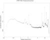 |
Fig. A.1 The spectrum of the background in the Chandra 4 Ms exposure of the CDFS. The spectrum has been extracted from a circle of 8 arcmin radius, after excluding 5 arcsec radius regions around all detected sources (10–20 arcsec for bright sources and extended sources). |
The low energy background spectrum peaks at ~0.5 keV and is quite dramatically lower between ~0.6 and ~1 keV. This continuum and the 0.585 line suggest that this part of the background spectrum is dominated by the thermal emission from the local “superbubble”. Below 0.3 keV, the response of the instrument decreases sharply and we therefore limited the analysis to energies above 0.3 keV.
We then fitted the background spectrum between 0.3 and 7 keV with a model including: 1) three Gaussian lines to account for the features at 1.48, 1.74, and 2.16 keV; 2) one broad Gaussian line to reproduce the broad bump between 1 and 3 keV; 3) two power laws modified at low energy by photoelectric absorption to reproduce the broad band hard continuum, all which were not convolved with the mirror effective area; and 4) a thermal component with abundances fixed to Solar values, that was convolved with the mirror effective area. This model provides a good fit to the background spectrum, without any systematic residuals. We then fitted the same model to the background spectra accumulated in three different regions, adjusting only the global normalizations of the model spectra accounting for the internal and cosmic background components. The fits are remarkably good above 1 keV. Below this energy, we see a deficit of counts in both the 3 arcmin radius spectrum and the 3–6 arcmin radius annulus spectrum, while there is an excess in the 6–8 arcmin annulus spectrum. The spectra become increasingly soft at large off-axis angles. The relative intensity of the thermal component is higher in the on-axis spectrum than the off-axis spectrum, as expected if this component is truly cosmic, because of the larger mirror vignetting at high off-axis angles. The increase of the strength of the low energy cut-off at smaller off-axis is then probably due to a thicker deposition of contaminants at the center of the ACIS-I 4 chip region.
The behavior observed for the emission lines is quite interesting. While the intensity of the 1.49 keV and 2.16 keV lines is constant with the off-axis angle, the intensity of the 1.78 keV Si line is larger at large off-axis angles.
The variations in the background spectra accumulated in thinner annuli becomes comparable to the statistical uncertainty. Guided by this analysis, we decided to adopt the average background spectra accumulated in the three r < 3′, 3′ < r < 6′, and 6′ < r < 8′ in the following analysis.
To evaluate the background counts in each source extraction region, we need to normalize the average background at three off-axis angles to that at each source position. We first extracted spectra from circular regions of 10 arcsec radii centered at each galaxy position, and then normalize the average background to that in these spectra using the 7–11 keV faint-source-free band. The statistical uncertainty in the background evaluation is therefore mostly given by the 7–11 keV total number of counts at the source position. The choice of the size of the extraction region at each galaxy position must then satisfy two competing requirements. On the one hand, the region must be large enough to provide enough counts to keep statistical fluctuation small. On the other hand, a small region has the advantage of avoiding systematic errors caused by sharp variations in the exposure time (and so of the background) typical of mosaics such as ACIS-I CDFS, cosmetic defects, and crowded regions with several sources within a few arcsec. The average CDFS 7–11 keV background in a 10 arcsec radius region is between 600 and 700 counts, ~ 3 times higher than the 0.5–2 keV average background, 4 times the 1–2 keV background, and 2 times the 1–4 keV background. Therefore, a circular region of 10 arcsec radius is a good compromise, because it collects a number of 7–11 keV counts similar to or higher than the 0.5–2, 1–2 or 1–4 keV counts in 10–20 arcsec annulus (a typical region used to extract a “local” background in crowded areas such as the CDFS), in a three times smaller area.
A.2. Completeness, reliability and sky coverage
To extract statistically quantitative information from a given sample of “detected” sources, we need to first assess its completeness and reliability (number of spurious detections). We performed a series of extensive detection runs on simulated data.
To assess the reliability of our survey, we first performed simulations using background spectra only. We simulated about 105 spectra at the positions of the sources detected in the CDFS to use exactly the same exposure time, vignetting, and PSF, but including only the average background at each off-axis position. We applied our version of ePhot to these simulations and studied the number of spurious detections as a function of various parameters: 1) the threshold on background-subtracted counts in a wide (0.3–4 keV) band; 2) the minimum and maximum source-extraction regions; 3) the energy grid used to search for detections; 4) the band-width Emax/Emin; and 5) the Poisson probability threshold for a source detection. We chose a combination of parameters that keeps the number of spurious detections smaller than one every 5000 spectra, i.e. the number of candidates in our search (see Sect. 2): these are 0.3–4 keV background-subtracted counts ≥ 12, Emax/Emin > 2, and Poisson probability < 2 × 10⁴.
To study the completeness of our survey, we performed detection runs on simulated source plus background spectra. We used mock X-ray catalogs generated by Gilli, which include about 105 AGN with a distribution of luminosities, redshifts, and absorbing column densities in accordance with the Gilli et al. CXB model. In particular, the mock catalogs include sources with unabsorbed flux down to 10-18 cgs, where the AGN density is ~20 000 deg2. Source spectra are distributed over six templates, with column densities NH up to 3 × 1024 cm-2. A pure reflection spectrum is also considered to account for heavily Compton thick sources. The distributions of spectra is a strong function of both luminosity and redshift (see Gilli et al. , for details). Using these mock catalogs, we simulated a 10 deg2Chandra survey with the same characteristics of the CDFS survey. We simulated sources at the position of the sources detected in the CDFS. We added to each simulated spectrum a background proportional to the average background at each off-axis angle. Finally, we run on each source + background simulated spectrum our source detection algorithm ePhot. These simulations are used to study the completeness of our survey and compute the corresponding sky coverage. In Fig. A.2, top panel, we compare the 0.5–2 keV observed flux histogram of the simulated sources with that of the sources detected by ePhot with the thresholds defined above. The ratio of the two histograms gives the completeness of our survey, or the sky coverage, when normalized to the CDFS searched area. Figure A.2, bottom panel, compares the ePhotsky coverage for the ERS area of the CDFS to that of a traditional detection algorithm at the same probability threshold (same fraction of spurious detections).
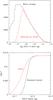 |
Fig. A.2 Top panel: the 0.5–2 keV flux histogram of the simulated sources (black solid histogram) and of the simulated sources detected by e-phot. Bottom panel: the Chandra sky coverage in the ERS area obtained using a standard detection algorithm (black solid curve) and using e-phot (red dashed curve) at the same probability threshold. |
A.3. Photometry
Our algorithm e-phot was also run on the galaxy samples with fixed energy bands (0.5–2 keV, thus optimizing only for the size of the source extraction region). The X-ray fluxes in the band 0.5–2 keV are estimated from e-phot count rates in the 0.5–2 keV band if the signal-to-noise ratio in this band is higher than 2.5 or from the count rates in the band that optimize the detection otherwise. A simple power-law spectrum with αE = 0.4 was assumed for the count rate flux conversion. To test our photometry, we compared the 0.5–2 keV flux obtained from the event files of the first 2 Ms observations to those in Luo08, and the 0.5–2 keV flux obtained form the full 4 Ms observations to those in Xue11. The agreement is remarkable, the median of the two samples agree to within 3% and the semi-interquartile range of their ratio is 0.06. Fluxes of faint detections can be statistically over-estimated because of the so-called Eddington bias (Hogg & Turner ; Wang ). We estimated the bias according to Wang and found that it is at most ~20% for our faintest detection and negligible for most of the Chandra-GOODS-ERS and Chandra-GOODS-MUSIC sources. Luminosities in Table 3 are calculated from fluxes that are corrected for the Eddington bias.
We do not discuss here the rest of the Chandra-GOODS-MUSIC sample because it is affected by incompleteness (see next section) and the quality of the photometric redshift is lower than that of the GOODS-ERS sample.
Assuming a Salpeter IMF would result in a SFR that is ~ 1.7 times higher.
Acknowledgments
This work was supported by ASI/INAF contracts I/024/05/0 and I/009/10/0. F.S. acknowledges support from the Alexander von Humboldt Foundation. We thank R. Gilli for providing us with his mock catalogs of X-ray sources based on the GCH2007 model. F.F. thanks G. C. Perola, A. Comastri, M. Brusa, F. La Franca, G. Melini, R. Maiolino, E. Giallongo, and H. Netzer for useful discussions. This work is based on observations made with the NASA X-ray observatory Chandra. We thank the Chandra director’s office for allocating the time for these observations. X-ray data were obtained from the archive of the Chandra X-ray Observatory Center, which is operated by the Smithsonian Astrophysical Observatory. This work is also based on data obtained with the NASA/ESA Hubble Space Telescope, obtained from the data archive at the Space Telescope Institute. STScI is operated by the association of Universities for Research in Astronomy, Inc. under the NASA contract NAS 5-26555. Observations were also carried out using the Very Large Telescope at the ESO Paranal Observatory under Programme IDs LP181.A-0717, ID 170.A-0788, and the ESO Science Archive under Programme IDs 67.A-0249, 71.A-0584, and 9.A-0539.
References
- Aird, J., Aird, J., Nandra, K., Laird, E. S., et al. 2010, MNRAS, 401, 2531 [NASA ADS] [CrossRef] [Google Scholar]
- Batcheldor, D. 2010, ApJ, 711, L108 [NASA ADS] [CrossRef] [Google Scholar]
- Barnes, J. E., & Hernquist, L. 1996, ApJ, 471, 115 [NASA ADS] [CrossRef] [Google Scholar]
- Begelman, M. C. 2010, MNRAS, 402, 673 [NASA ADS] [CrossRef] [Google Scholar]
- Best, P. N., Kauffmann, G., Heckman, T. M., et al. 2005, MNRAS, 362, 35 [Google Scholar]
- Boutsia, K., Boutsia, K., Grazian, A., Giallongo, E., et al. 2011, ApJ, 736, 41 [NASA ADS] [CrossRef] [Google Scholar]
- Bouwens, R. J., Illingworth, G. D., Blakeslee, J. P., & Franx, M. 2006, ApJ, 653, 53 [NASA ADS] [CrossRef] [Google Scholar]
- Bouwens, R. J., Bouwens, R. J., Illingworth, G. D., Oesch, P. A., et al. 2011, ApJ, 737, 90 [NASA ADS] [CrossRef] [Google Scholar]
- Brandt, W. N., Vignali, C., Schneider, D. P., et al. 2004, Adv. Space Res., 34, 2478 [NASA ADS] [CrossRef] [Google Scholar]
- Brusa, M., Comastri, A., Gilli, R., et al. 2009a, ApJ, 693, 8 [NASA ADS] [CrossRef] [Google Scholar]
- Brusa, M., Fiore, F., Santini, P., et al. 2009b, A&A, 507, 1277 [NASA ADS] [CrossRef] [EDP Sciences] [Google Scholar]
- Brusa, M., Fiore, F., Santini, P., et al. ApJ, 2010, 716, 348 [Google Scholar]
- Bundy, K., Georgakakis, A., Nandra, K., et al. 2008, ApJ, 681, 931 [NASA ADS] [CrossRef] [Google Scholar]
- Calzetti, D., Armus, L., Bohlin, R. C., et al. 2000, ApJ, 533, 682 [NASA ADS] [CrossRef] [Google Scholar]
- Caputi, K. I., Cirasuolo, M., Dunlop, J. S., et al. 2011, MNRAS, 413, 162 [NASA ADS] [CrossRef] [Google Scholar]
- Castellano, M., Fontana, A., Paris, D., et al. 2010, A&A, 524, A28 [NASA ADS] [CrossRef] [EDP Sciences] [Google Scholar]
- Cardamone, C. N., van Dokkum, P. G., Urry, C. M., et al. 2010, ApJS, 189, 270 [NASA ADS] [CrossRef] [Google Scholar]
- Cavaliere, A., & Vittorini, V. 2000, ApJ, 543 599 [Google Scholar]
- Cen, R. 2011, ApJ, submitted [arXiv:1102.0262] [Google Scholar]
- Ciotti, L., & Ostriker, J. P. 2007, ApJ, 665, 1038 [NASA ADS] [CrossRef] [Google Scholar]
- Ciotti, L., Ostriker, J. P., & Proga, D. 2010, ApJ, 717, 708 [NASA ADS] [CrossRef] [Google Scholar]
- Civano, F., Brusa, M., Comastri, A., et al. 2011, ApJ, 741, 91 [NASA ADS] [CrossRef] [Google Scholar]
- Comastri, A., Ranalli, P., Iwasawa, K., et al. 2011, A&A, 526, L9 [NASA ADS] [CrossRef] [EDP Sciences] [Google Scholar]
- Cowie, L. L., Barger, A. J., & Hu, E. M. 2010, ApJ, 711, 928 [NASA ADS] [CrossRef] [Google Scholar]
- Daddi, E., Alexander, D. M., Dickinson, M., et al. 2007, ApJ, 670, 173 [NASA ADS] [CrossRef] [Google Scholar]
- Dotti, M., Volonteri, M., Perego, A., et al. 2010, MNRAS, 402, 682 [NASA ADS] [CrossRef] [Google Scholar]
- Ebrero, J., Carrera, F. J., Page, M. J., et al. 2009, A&A, 493, 55 [NASA ADS] [CrossRef] [EDP Sciences] [Google Scholar]
- Fanidakis, N., Baugh, C. M., Benson, A. J., et al. 2011, MNRAS, 410, 53 [NASA ADS] [CrossRef] [Google Scholar]
- Feruglio, C., Daddi, E., Fiore, F., et al. 2011, ApJ, 729, L4 [NASA ADS] [CrossRef] [Google Scholar]
- Ferrarese, L., & Ford, H. 2005, Space Sci. Rev., 116, 523 [NASA ADS] [CrossRef] [Google Scholar]
- Fiore, F. 2010, AIP Conf. Proc., 1248, 373 [NASA ADS] [CrossRef] [Google Scholar]
- Fiore, F., Brusa, M., Cocchia, F., et al. 2003, A&A, 409, 79 [NASA ADS] [CrossRef] [EDP Sciences] [Google Scholar]
- Fiore, F., Grazian, A., Santini, P., et al. 2008, ApJ, 672, 94 [NASA ADS] [CrossRef] [Google Scholar]
- Fiore, F., Puccetti, S., Brusa, M., et al. 2009 ApJ, 693, 447 [Google Scholar]
- Fiore, F., Puccetti, S., & Mathur, S. 2011, Adv. Astron., in press [arXiv:1109.4586] [Google Scholar]
- Fontana, A., Salimbeni, S., Grazian, A., et al. 2006, A&A, 459, 745 [NASA ADS] [CrossRef] [EDP Sciences] [Google Scholar]
- Fontanot, F., Cristiani, S., Monaco, P., et al. 2007, A&A, 461, 39 [NASA ADS] [CrossRef] [EDP Sciences] [Google Scholar]
- Gallerani, S., Maiolino, R., Juarez, Y., et al. 2010, A&A, 523, A85 [NASA ADS] [CrossRef] [EDP Sciences] [Google Scholar]
- Georgantopoulos, I., Akylas, A., Georgakakis, A., & Rowan-Robinson, M. 2009, A&A, 507, 747 [NASA ADS] [CrossRef] [EDP Sciences] [Google Scholar]
- Georgantopoulos, I., Rovilos, E., Xilouris, E. M., Comastri, A., & Akylas, A. 2011, A&A, 526, A86 [NASA ADS] [CrossRef] [EDP Sciences] [Google Scholar]
- Genzel, R., Tacconi, L. J., Eisenhauer, F., et al. 2006, Nature, 442, 786 [NASA ADS] [CrossRef] [PubMed] [Google Scholar]
- Giacconi, R., Zirm, A., Wang, J., et al. 2002, ApJS, 139, 369 [NASA ADS] [CrossRef] [Google Scholar]
- Giallongo, E., Fontana, A., & Madau, P. 1997, MNRAS, 289, 629 [NASA ADS] [Google Scholar]
- Gilli, R., Comastri, A., & Hasinger, G. 2007, A&A 463, 79 [NASA ADS] [CrossRef] [EDP Sciences] [Google Scholar]
- Gilli, R., Su, J., Norman, C., et al. 2011, ApJ, 730, L28 [NASA ADS] [CrossRef] [Google Scholar]
- Glikman, E., Djorgavski, S. G., Stern, D., et al. 2011, ApJ, 728, L26 [NASA ADS] [CrossRef] [Google Scholar]
- Graham, A. W., Onken, C. A., Athanassoula, E., & Combes, F. 2011, MNRAS, 412, 2211 [NASA ADS] [CrossRef] [Google Scholar]
- Grogin, N. A., Kocevski D. D., Faber S. M., et al. 2011, ApJS, submitted [arXiv:1105.3753] [Google Scholar]
- Grazian, A., Fontana, A., de Santis, C., et al. 2006, A&A, 449, 951 [NASA ADS] [CrossRef] [EDP Sciences] [Google Scholar]
- Grazian, A., Castellano, M., Koekemoer, A. M., et al. 2011, A&A, 532, A33 [NASA ADS] [CrossRef] [EDP Sciences] [Google Scholar]
- Haring, N., & Rix, H.-W. 2004, ApJ, 604, L89 [NASA ADS] [CrossRef] [Google Scholar]
- Hogg, D. W., & Turner, E. L. 1998, PASP, 110, 727 [NASA ADS] [CrossRef] [Google Scholar]
- Hopkins, P. F., Hernquist, L., Cox, T. J., et al. 2006, ApJS, 163, 1 [Google Scholar]
- Hopkins, P. F., Richards, G. T., & Hernquist, L. 2007, ApJ, 654, 731 [NASA ADS] [CrossRef] [Google Scholar]
- Jiang, L., Fan, X., Hines, D. C., et al. 2006, AJ, 132, 2127 [NASA ADS] [CrossRef] [Google Scholar]
- Jiang, L., Fan, X., Bian, F., et al. 2009, AJ, 138, 305 [NASA ADS] [CrossRef] [Google Scholar]
- Kauffmann, G., & Heckman, T. M. 2009, MNRAS, 397, 135 [NASA ADS] [CrossRef] [Google Scholar]
- Kauffmann, G., Heckman, T. M., Tremonti, C., et al. 2003, MNRAS, 346, 1055 [Google Scholar]
- Kelly, B. C., Vestergaad, M., Fan, X., et al. 2010, ApJ, 719, 1315 [NASA ADS] [CrossRef] [Google Scholar]
- King, A. R., Pringle, J. E., & Hofmann, J. A. 2008, MNRAS, 385, 1621 [NASA ADS] [CrossRef] [Google Scholar]
- Koekemoer, A. M., Faber S. M., C. F. Henry, et al. 2011, ApJS, submitted [arXiv:1105.3754] [Google Scholar]
- Kollmeier, J. A., Onken, C. A., Kochanek, C. S., et al. 2006, ApJ, 648, 128 [NASA ADS] [CrossRef] [Google Scholar]
- Krumholz, M. R., & Dekel, A. 2011, ApJ, submitted [arXiv:1106:0301] [Google Scholar]
- La Franca, F., Fiore, F., Comastri, A., et al. 2005, ApJ, 635, 864 [NASA ADS] [CrossRef] [Google Scholar]
- La Franca, F., Melini, G., & Fiore, F. 2010, ApJ, 718, 368 [NASA ADS] [CrossRef] [Google Scholar]
- Lamastra, A., Menci, N., Maiolino, R., Fiore, F., & Merloni, A. 2010, MNRAS, 405, 29 [NASA ADS] [Google Scholar]
- Lamastra, A., Menci, N., Fiore, F., Di Porto, C., & Amendola, L. 2011, MNRAS, in press [arXiv:1111.3800] [Google Scholar]
- Lapi, A., Cavaliere, A., & Menci, N. 2005, ApJ, 619, L60 [NASA ADS] [CrossRef] [Google Scholar]
- Lapi, A., Shankar, F., Mao, J., et al. 2006, ApJ, 650, 42 [NASA ADS] [CrossRef] [Google Scholar]
- Lodato, G., & Natarajan, P. 2006, MNRAS, 371, 1813 [NASA ADS] [CrossRef] [Google Scholar]
- Lodato, G., & Natarajan, P. 2007, MNRAS, 377, L64 [NASA ADS] [Google Scholar]
- Luo, B., Bauer, F. E., Brandt, W. N., et al. 2008, ApJS 179, 19 (Luo08) [Google Scholar]
- Luo, B., Brandt, W. N., Xue, Y. Q., et al. 2010, ApJS 187, 560 (Luo10) [Google Scholar]
- Madau, P., & Rees, M. J. 2001, ApJ, 551, L27 [NASA ADS] [CrossRef] [Google Scholar]
- Malkan, M., Webb, W., & Konopacky, Q. 2003, ApJ, 598, 878 [NASA ADS] [CrossRef] [Google Scholar]
- Marconi, A., Risaliti, G., Gilli, R., et al. 2004, MNRAS 351, 169 [Google Scholar]
- Maiolino, R., Marconi, A., Salvati, M., et al. 2001, A&A, 365, 28 [NASA ADS] [CrossRef] [EDP Sciences] [Google Scholar]
- Maiolino, R., Schneider, R., Oliva, E., et al. 2004, Nature, 431, 533 [NASA ADS] [CrossRef] [PubMed] [Google Scholar]
- Maiolino, R., Nagao, T., Grazian, A., et al. 2008, A&A, 488, 463 [NASA ADS] [CrossRef] [EDP Sciences] [Google Scholar]
- Malizia, A., Stephen, J. B., Bassani, L., et al. 2009, MNRAS, 399, 944 [NASA ADS] [CrossRef] [Google Scholar]
- Mathur, S., Kuraszkiewicz, J., & Czerny, B. 2001, New Astron., 6, 321 [NASA ADS] [CrossRef] [Google Scholar]
- Mathur, S., Wilkes, B. J., & Gosh, H. 2002, ApJ, 570, L5 [NASA ADS] [CrossRef] [Google Scholar]
- Mathur, S., Fields, D., Peterson, B. M., Grupe, D., et al. 2011, ApJ, submitted [arXiv:1102.0537] [Google Scholar]
- McLure, R. J., Dunlop, J. S., Cirasuolo, M., et al. 2010, MNRAS, 403, 960 [NASA ADS] [CrossRef] [Google Scholar]
- McLure, R. J., Dunlop, J. S., de Ravel, L., et al. 2011, MNRAS, in press [arXiv:1102.4881] [Google Scholar]
- Menci, N., Cavaliere, A., Fontana, A., et al. 2004, ApJ, 604, 12 [NASA ADS] [CrossRef] [Google Scholar]
- Menci, N., Fontana, A., Giallongo, E., Grazian, A., & Salimbeni, S. 2006, ApJ, 647, 753 [NASA ADS] [CrossRef] [Google Scholar]
- Menci, N., Fiore, F., Puccetti, S., & Cavaliere, A. 2008, ApJ, 686, 219 [NASA ADS] [CrossRef] [Google Scholar]
- Merloni, A., & Heinz, S. 2008, MNRAS, 388, 1011 [NASA ADS] [Google Scholar]
- Merloni, A., Rudnick, G., & Di Matteo, T. 2004, MNRAS, 354, L37 [NASA ADS] [CrossRef] [Google Scholar]
- Miller, N. A., Fomalont, E. B., Kellermann, K. I., et al. 2008, ApJS, 179, 114 [NASA ADS] [CrossRef] [Google Scholar]
- Netzer, H. 2009a, ApJ, 695, 793 [NASA ADS] [CrossRef] [Google Scholar]
- Netzer H. 2009b, MNRAS, 399, 1907 [NASA ADS] [CrossRef] [Google Scholar]
- Netzer, H., & Trakhtenbrot, B. 2007, ApJ, 654, 754 [NASA ADS] [CrossRef] [Google Scholar]
- Norman, C., Hasinger, G., Giacconi, R., et al. 2002, ApJ 571, 218 [Google Scholar]
- Padovani, P., Miller, N., Kellermann, K. I., et al. 2011, ApJ, 740, 20 [NASA ADS] [CrossRef] [Google Scholar]
- Panessa, F., Bassani, L., Cappi, M., et al. 2006, A&A, 455, 173 [NASA ADS] [CrossRef] [EDP Sciences] [Google Scholar]
- Pannella, M., Carilli, C. L., Daddi, E., et al. 2009, ApJ, 698, L116 [Google Scholar]
- Piconcelli, E., Bianchi, S., Guainazzi, M., Fiore, F., & Chiaberge, M. 2007, A&A, 466, 855 [NASA ADS] [CrossRef] [EDP Sciences] [Google Scholar]
- Primack, J. R. 2009, AIP Conf. Proc., 1192, 101 [NASA ADS] [CrossRef] [Google Scholar]
- Ranalli, P., Comastri, A., & Setti, G. 2003, A&A, 399, 39 [NASA ADS] [CrossRef] [EDP Sciences] [Google Scholar]
- Richards, G. T., Lacy, M., Storrie-Lombardi, L. J., et al. 2006, ApJS, 166, 470 [NASA ADS] [CrossRef] [Google Scholar]
- Risaliti, G., Maiolino, R., & Salvati, M. 1999, ApJ, 522, 157 [NASA ADS] [CrossRef] [Google Scholar]
- Risaliti, G., Elvis, M., Fabbiano, G., Baldi, A., & Zezas, A. 2005, ApJ, 623, L93 [NASA ADS] [CrossRef] [Google Scholar]
- Schmidt, M. 1968, ApJ, 151, 393 [NASA ADS] [CrossRef] [Google Scholar]
- Santini, P., Fontana, A., Grazian, A., et al. 2009, A&A, 504, 751 [NASA ADS] [CrossRef] [EDP Sciences] [Google Scholar]
- Santini, P., Fontana, A., Grazian, A., et al. 2011, A&A, in press DOI: 10.1051/0004-6361/201117513 [Google Scholar]
- Shen, Y. 2009, ApJ, 697, 1656 [NASA ADS] [CrossRef] [Google Scholar]
- Shankar, F. 2009, New A Rev., 53, 57 [Google Scholar]
- Shankar, F. 2010, IAU Symp., 267, 248 [NASA ADS] [Google Scholar]
- Shankar, F., & Mathur, S. 2007, ApJ, 660, 1051 [NASA ADS] [CrossRef] [Google Scholar]
- Shankar, F., Weinberg, D. H., & Miralda-Escudé, J. 2009a, ApJ, 690, 20 [NASA ADS] [CrossRef] [Google Scholar]
- Shankar, F., Bernardi, M., & Haiman, Z. 2009b, ApJ, 694, 867 [NASA ADS] [CrossRef] [Google Scholar]
- Shankar, F., Crocce, M., Miralda-Escudé, J., Fosalba, P., & Weinberg, D. H. 2010a, ApJ, 718, 231 [NASA ADS] [CrossRef] [Google Scholar]
- Shankar, F., Weinberg, D. H., & Shen, Y. 2010b, MNRAS, 406, 1959 [NASA ADS] [Google Scholar]
- Shemmer, O., Netzer, H., Maiolino, R., et al. 2004, ApJ, 614, 547 [NASA ADS] [CrossRef] [Google Scholar]
- Shemmer, O., Brandt, W. N., Schneider, D. P., et al. 2006, ApJ, 644, 86 [NASA ADS] [CrossRef] [Google Scholar]
- Shen, Y. 2009, ApJ, 704, 89 [NASA ADS] [CrossRef] [Google Scholar]
- Shi, Y., Rieke, G. H., Hines, D. C., et al. 2006, ApJ, 653, 127 [NASA ADS] [CrossRef] [Google Scholar]
- Stark, D. P., Ellis, R. S., Bunker, A., et al. 2009, ApJ, 697, 1493 [NASA ADS] [CrossRef] [Google Scholar]
- Trakhtenbrot, B., Netzer, H., Lira, P., & Shemmer, O. 2011, ApJ, 730, 7 [NASA ADS] [CrossRef] [Google Scholar]
- Treister, E., Urry, C. M., Schawinski, K., et al. 2010, ApJ, 722, L238 [NASA ADS] [CrossRef] [Google Scholar]
- Treister, E., Schawinski, K., Volonteri, M., Natarajan, P., & Gawiser, E. 2011, Nature, 474, 356 [NASA ADS] [CrossRef] [Google Scholar]
- Turner, T. J., George, I. M., Nandra, K., & Mushotzky, R. F. 1997, ApJS, 113, 23 [NASA ADS] [CrossRef] [Google Scholar]
- van der Wel, A., Rix, H.-W., Wuyts, S., et al. 2011, ApJ, 730, 38 [NASA ADS] [CrossRef] [Google Scholar]
- Viel, M., Becker, G. D., Bolton, J. S., et al. 2008, Phys. Rev. Lett., 100, 1304 [Google Scholar]
- Volonteri, M. 2010, A&ARv, 18, 279 [NASA ADS] [CrossRef] [Google Scholar]
- Volonteri, M., & Begelman, M. C. 2010, MNRAS, 409, 1022 [NASA ADS] [CrossRef] [Google Scholar]
- Volonteri, M., & Rees, M. J. 2005, ApJ, 633, 624 [NASA ADS] [CrossRef] [Google Scholar]
- Volonteri, M., Lodato, G., & Natarajan, P. 2008, MNRAS, 383, 1079 [NASA ADS] [CrossRef] [Google Scholar]
- Volonteri, M., Natarajan, P., & Gultekin, K. 2011, ApJ, 727, 50 [NASA ADS] [CrossRef] [Google Scholar]
- Wang, Q. D. 2004, ApJ, 612, 159 [NASA ADS] [CrossRef] [Google Scholar]
- Willott, C. J. 2011, ApJ, 742, L8 [NASA ADS] [CrossRef] [Google Scholar]
- Willott, C. J., Delorme, P., Reylé, C., et al. 2010a, AJ, 139, 906 [NASA ADS] [CrossRef] [Google Scholar]
- Willott, C. J., Albert, L., Arzoumanian, D., et al. 2010b, AJ, 140, 546 [NASA ADS] [CrossRef] [Google Scholar]
- Windhorst, R. A., Cohen, S. H., Hathi, N. P., et al. 2011, ApJS, 193, 27 [NASA ADS] [CrossRef] [Google Scholar]
- Wyithe, J. S. B., & Loeb, A. 2003, ApJ, 595, 614 [NASA ADS] [CrossRef] [Google Scholar]
- Xue, Y. Q., Luo, B., Brandt, W. N., et al. 2011, ApJS, 195, 10 (Xue11) [NASA ADS] [CrossRef] [Google Scholar]
- Yamada, T., Kajisawa, M., Akiyama, M., et al. 2009, ApJ, 699, 1354 [NASA ADS] [CrossRef] [Google Scholar]
- Yun, M. S., Reddy, N. A., & Condon, J. J. 2001, ApJ, 554, 803 [NASA ADS] [CrossRef] [Google Scholar]
All Tables
All Figures
|
Fig. 1 HST ACS B band (left panel), z band (central panel) and HST WFC3 H band (right panel) images of three Chandra-GOODS-ERS sources with overlaid X-ray contours in the 0.7–2.7 keV band (E2199), 0.7–1.9 keV band (E2551) and 0.4–1.5 keV band (E4956). |
| In the text | |
|
Fig. 2 The Chandra X-ray spectra of E537 (Left panel), E1577 (central panel), and M 4835 (right panel). |
| In the text | |
|
Fig. 3 The best-fit NH as a function of the 0.16 μm extinction for the 10 z > 3 highly obscured or Compton thick AGN. Filled points are sources with point-like optical or near infrared morphology. The two solid lines are the expectation for a dust-to-gas ratio 100 and 1000 times lower than the Galactic one. |
| In the text | |
|
Fig. 4 K band, MIPS 24 μm, and LABOCA 870 μm images around the M 4417 galaxy with overlaid X-ray 0.5–3.2 keV contours. |
| In the text | |
|
Fig. 5 Left panel: the X-ray to NIR flux ratio F(0.5–2 keV)/F(H) as a function of the X-ray flux for the z > 3 Chandra-GOODS-ERS AGN sample (red-filled circles), Chandra-GOODS-MUSIC sample (black-open circles), Chandra-COSMOS sample (green-filled squares) and XMM-COSMOS sample (blue-filled triangles. Right panel: the distributions of F(0.5–2 keV)/F(H) for the Chandra-COSMOS z > 3 sample (black histogram), Chandra-ERSVO sample (red histogram), and Chandra-GOODS-MUSIC sample (blue, dashed histogram). |
| In the text | |
|
Fig. 6 The UV 1450 Å to X-ray 2–10 keV luminosity ratio for 12 QSOs at z > 5.7. |
| In the text | |
|
Fig. 7 The AGN 2–10 keV luminosity functions at z = 3–4 (top panel), z = 4–5 (central panel), and z > 5.8 (bottom panel). Large red-filled circles are from the CDFS Chandra-GOODS-MUSIC and Chandra-GOODS-ERS samples. Red-filled triangles are from Chandra-COSMOS (Civano et al. 2011), red-filled squares from XMM-COSMOS (Brusa et al. 2010). The blue thick curve in the top panel is the LADE model of Aird et al. (2010) in the 2.5–3.5 redshift bin. Large black-open triangles are SDSS data from Richards et al. (2006), stars are SDSS data from Jiang et al. (2009), open circles are from Glikman et al. (2011), and small blue-open triangles are from Fontanot et al. (2007). Black dashed curves are best fits to the X-ray plus optical, wide-luminosity-range luminosity functions (see text for details). Magenta solid curves encompass the predictions of the Menci et al. (2006, 2008) semi-analytic model. Blue curves are models from Shankar et al. (2011, see the Discussion for details). |
| In the text | |
|
Fig. 8 Top panel: a collection of AGN luminosity functions at z ≲ 2 from La Franca et al. (2005), and z > 3 in this work. Central panel: SMBH mass functions obtained by combining the AGN luminosity functions in the top panel with Eddington ratio distributions (see the text for details). Bottom panel: a collection of galaxy stellar mass functions. z ≲ 2 from Fontana et al. (2006), z = 3–4 from Santini et al. (2011), z = 4–5 from Caputi et al. (2011), and z = 6 from Stark et al. (2009). |
| In the text | |
|
Fig. 9 Top panel: the AGN duty cycle as a function of the galaxy stellar mass in six redshift bins. AGN with log L(2–10 keV) > 43 are considered only. Bottom panel: the AGN duty cycle as a function of redshift for two galaxy stellar masses (log M∗ = 11.25, 11.75 M⊙). Filled circles and triangles are the previous determination of Brusa et al. (2009b) for the same masses. The black dashed (dotted) curve is the prediction of the Menci et al. (2006, 2008) SAM for log M∗ = 11.25 M⊙ (log M∗ = 10 M⊙). |
| In the text | |
|
Fig. A.1 The spectrum of the background in the Chandra 4 Ms exposure of the CDFS. The spectrum has been extracted from a circle of 8 arcmin radius, after excluding 5 arcsec radius regions around all detected sources (10–20 arcsec for bright sources and extended sources). |
| In the text | |
|
Fig. A.2 Top panel: the 0.5–2 keV flux histogram of the simulated sources (black solid histogram) and of the simulated sources detected by e-phot. Bottom panel: the Chandra sky coverage in the ERS area obtained using a standard detection algorithm (black solid curve) and using e-phot (red dashed curve) at the same probability threshold. |
| In the text | |
Current usage metrics show cumulative count of Article Views (full-text article views including HTML views, PDF and ePub downloads, according to the available data) and Abstracts Views on Vision4Press platform.
Data correspond to usage on the plateform after 2015. The current usage metrics is available 48-96 hours after online publication and is updated daily on week days.
Initial download of the metrics may take a while.