| Issue |
A&A
Volume 536, December 2011
|
|
|---|---|---|
| Article Number | A34 | |
| Number of page(s) | 17 | |
| Section | Cosmology (including clusters of galaxies) | |
| DOI | https://doi.org/10.1051/0004-6361/201117522 | |
| Published online | 05 December 2011 | |
The red-sequence of 72 WINGS local galaxy clusters
1
Astronomy DepartmentUniversity of Padova, Vicolo Osservatorio 2, 35122 Padova, Italy
2
INAF – Padova Astronomical Observatory, Vicolo Osservatorio 5, 35122 Padova, Italy
e-mail: This email address is being protected from spambots. You need JavaScript enabled to view it.
3
INAF – Trieste Astronomical Observatory, via Tiepolo 11, 34131 Trieste, Italy
4
Sterrenkundig Observatorium Vakgroep Fysica en Sterrenkunde Universeit Gent, Gent, Belgium
5
Centro de Estudios de Física del Cosmos de Aragón, Plaza de San Juan 1, 44001 Teruel, Spain
6
Centre for Astrophysics & Supercomputing, Swinburne University, Hawthorn 3122, VIC, Australia
7
Observatories of the Carnegie Institution of Washington, Pasadena, CA 91101, USA
8
The Niels Bohr Institute, Juliane Maries Vej 30, 2100 Copenhagen, Denmark
9
Departamento de Astrofisica, Universidad Complutense de Madrid, Spain
Received: 20 June 2011
Accepted: 16 September 2011
Abstract
We study the color − magnitude red sequence and blue fraction of 72 X-ray selected galaxy clusters at z = 0.04−0.07 from the WINGS survey, searching for correlations between the characteristics of the red sequence (RS) and the environment. We consider the slope and scatter of the red sequence, the number ratio of red luminous-to-faint galaxies, the blue fraction, and the fractions of ellipticals, S0s, and spirals that compose the RS. None of these quantities correlate with the cluster velocity dispersion, X-ray luminosity, number of cluster substructures, BCG prevalence over next brightest galaxies, and the spatial concentration of ellipticals. The properties of the RS, instead, depend strongly on local galaxy density. Higher density regions have a smaller RS scatter, a higher luminous-to-faint ratio, a lower blue fraction, and a lower spiral fraction on the RS. Our results clearly illustrate the prominent effect of the local density in setting the epoch when galaxies become passive and join the red sequence, as opposed to the mass of the galaxy host structure.
Key words: galaxies: clusters: general / galaxies: evolution / galaxies: stellar content / galaxies: elliptical and lenticular, cD / galaxies: fundamental parameters
© ESO, 2011
1. Introduction
The location of galaxies in a color-absolute magnitude diagram has traditionally been one of the most useful methods to examine the stellar population properties of galaxies and their evolution.
The importance of the color − magnitude diagram in galaxy studies can hardly be overstated. Very early studies (de Vaucouleurs 1961; Visvanathan & Sandage 1977) recognized the existence in such a diagram of a red sequence, consisting primarily of early-type galaxies, which is also known as the “color − magnitude relation” (CMR) because it represents a positive correlation between galaxy color and luminosity.
The RS is an easily recognizable feature in the color–magnitude diagram that can be used, to first approximation, to separate red, passively evolving galaxies devoid of star formation, from bluer star-forming galaxies. Innumerable studies have investigated the origin of this relation, and the reasons why a galaxy either belongs to it, or falls below it at bluer colors.
The slope, scatter, and location of the RS have long been used to place constraints on the formation epoch of stars in early-type galaxies (Bower et al. 1992; Ellis et al. 1997; Kodama et al. 1998). The RS is most conspicuous in galaxy clusters, which are rich in passive early-type galaxies. A well-defined RS has been observed in clusters up to high redshifts (Lidman et al. 2008; Mei et al. 2009; Strazzullo et al. 2010) and the knowledge that the galaxies with the oldest stars preferentially inhabit clusters at any epoch can be used to identify galaxy clusters, using their RS, up to high redshifts (Gladders & Yee 2005; Muzzin et al. 2009; Wilson et al. 2009; Gilbank et al. 2011).
Observations of the relative fractions of galaxies on and below the RS have uncovered evolution in the star formation activity within clusters (Butcher & Oemler 1984; Ellingson et al. 2001; Loh et al. 2008) and, more recently, in the field (Bell et al. 2004; Faber et al. 2007; Bell et al. 2007). It has thus become clear that a large number of galaxies have stopped forming stars and have turned from blue to red at z below 1 in all environments, but in a way that depends on environment. It is also now well-established that this progressive “passivization” process of galaxies proceeds in a downsizing fashion, with more massive and luminous galaxies reaching the RS at earlier epochs than lower-mass, fainter galaxies (Cowie et al. 1996). Large spectroscopic surveys have confirmed and placed on a very solid statistical ground earlier results on the correspondence between the bimodality in colors (red and blue) and other main galaxy characteristics such as morphological type (early and late) and galaxy stellar mass (Strateva et al. 2001; Kauffmann et al. 2003; Cheng et al. 2011).
One of the main outstanding questions remains the physical reason why galaxies stop forming stars and become red. Naturally, there can be multiple physical mechanisms responsible for the end of star formation. Their relative importance might vary with galaxy mass, galaxy location (environment), and redshift, among other things (Peng et al. 2010).
Two mechanisms in particular have been the subject of extensive theoretical investigation in the past few years: AGN quenching and strangulation that causes the hot gas reservoir to be removed from galaxies upon merging with a larger halo (Croton et al. 2006; Bower et al. 2006; van den Bosch et al. 2008; Guo et al. 2011; McCarthy et al. 2010). Models however are currently unable to reproduce the observed trends, and generally overproduce the fraction of red galaxies (Font et al. 2008; Balogh et al. 2009; Kimm et al. 2009). In clusters, additional mechanisms are expected and observed to take place, such as ram pressure stripping (Gunn & Gott 1972) and harassment (Moore et al. 1998), though they may be much more efficient than originally thought even in lower mass systems than clusters (Bekki 2009).
The main issue is clearly to what extent the end of star formation is due to internal galaxy properties, or is related to either the global environment (for example the halo mass of the galaxy host structure) or the local environment. In this paper, we investigate the relation between the RS properties of galaxies in clusters and the global and local environmental properties in the local Universe. We use a survey of 77 X-ray selected nearby galaxy clusters (the WIde-field Nearby Galaxy-cluster Survey, WINGS)1 to search for correlations between the RS characteristics and the galaxy environment, with the aim of shedding some light on the mechanisms that produce the population of passive red galaxies in clusters today. The WINGS clusters span a wide range of cluster masses, and their galaxies are found at widely different local environmental densities, thus allowing a broad investigation using a homogeneous, high quality photometric dataset.
In Sects. 2 and 3, we describe the WINGS dataset and the method used to define the RS, respectively. In Sect. 4, we investigate whether the RS characteristics (slope, scatter, and value of the best-fit line at MV = −20), the ratio of the number of luminous to faint galaxies on the RS, the blue galaxy fraction, and the morphological fractions of galaxies on the RS depend on general cluster properties (cluster velocity dispersion, X-ray luminosity, BCG dominance, number of substructures, and concentration of ellipticals). We then study the same characteristics of the RS as a function of local galaxy density (Sect. 4.5). Our conclusions are summarized in Sect. 5.
Throughout this paper, we use the cosmological parameters (H0, Ωm, Ωλ) = (70 km s-1 Mpc-1, 0.3, 0.7).
2. The data
The galaxies examined in this paper are part of the multiwavelength survey WINGS (Fasano et al. 2006). WINGS is designed to provide a robust characterization of the photometric and spectroscopic properties of galaxies in nearby clusters, and to determine the variations in these properties as a function of galaxy mass and environment.
Clusters were selected in the X-ray from the ROSAT brightest cluster sample and its extension (Ebeling et al. 1998, 2000) and the X-ray brightest Abell-type cluster sample (Ebeling et al. 1996). The WINGS clusters cover a wide range of velocity dispersion σclus, typically between 500 and 1100 km s-1, and X-ray luminosity LX, typically 0.2 − 5 × 1044 erg/s.
The survey core dataset, consisting of optical B and V imaging of 78 nearby (0.04 < z < 0.07) galaxy clusters (Varela et al. 2009), has been complemented by several ancillary projects: (i) a spectroscopic follow up of about 6500 galaxies in a subsample of 48 clusters, obtained with the spectrographs WYFFOS at the WHT and 2dF at the AAT (Cava et al. 2009); (ii) near-infrared (J, K) imaging of a subsample of 28 clusters obtained with WFCAM at the UKIRT (Valentinuzzi et al. 2009); (iii) U broad- and Hα narrow-band imaging of subsamples of WINGS clusters, obtained with wide-field cameras at different telescopes (INT, LBT, Bok, see Omizzolo et al., in prep.).
The B and V photometric catalogs used in this paper are described in detail in (Varela et al. 2009). Briefly, our catalogs are 90% complete at V ~ 21.7, and the star-galaxy separation was visually checked, which ensures that the number of misclassifications was negligible, to as faint as V = 22. The distance moduli of our clusters are in the range 36.1 − 37.4, hence our photometric catalogs are highly complete and reliable down to MV = −15.7 or fainter. The photometry was performed on images in which large galaxies and halos of bright stars were removed after modeling them with elliptical isophotes. This procedure greatly improved the photometry of the large galaxies and increased the detection rate of objects projected onto them by 16% (Varela et al. 2009).
The WINGS galaxy morphologies were derived from V images using the purposely devised tool MORPHOT (Fasano et al. 2011; and Appendix A in Fasano et al. 2010). Our approach is a generalization of the non-parametric method proposed by Conselice (2000, see also Conselice 2003). In particular, we extended the classical CAS (Concentration/ Asymmetry/clumpinesS) parameter set by introducing a number of additional, suitably devised morphological indicators, using a final set of 11 parameters. A control sample of 1000 visually classified galaxies were used to calibrate the whole set of morphological indicators, with the aim of identifying the best sub-set among them, as well as analyzing how they depend on galaxy size, flattening, and signal-t-noise ratio. The morphological indicators were combined with two independent methods, a maximum likelihood analysis and a neural network trained on the control sample of visually classified galaxies. The final, automatic morphological classification combines the results of both methods. We verified that our automatic morphological classification closely reproduces the visual classification of two of us (AD and GF). In particular, the robustness and reliability of the MORPHOT results are comparable to those for the visual classifications obtained by different experienced human classifiers (Fasano et al., in prep.).
All of the following analysis is carried out for galaxies within R200/2, where R200 (usually considered an approximation of the cluster virial radius) is the radius enclosing the sphere with interior mean density 200 times the critical density of the Universe at that redshift. The R200/2 values were measured from the cluster velocity dispersions given in Table 1 as  (1)After careful visual inspection of all the B − V versus V color − magnitude diagrams (CMDs) of our clusters, we decided to consider only 72 clusters in our present study because of incomplete radial coverage out to R200/2 or a nearly absent RS.
Cluster properties.
In Table 1, we present a number of global properties of our clusters. Cluster redshifts are those from from Cava et al. (2009). Cluster velocity dispersions were derived, following the recipes given in Cava et al. (2009), from the WINGS database that collects, together with our data, all the available redshifts from NED. The X-ray total luminosities were taken from Ebeling et al. (1996, 1998, 2000) andconverted to our adopted cosmology. The number of substructures found in each cluster are drawn from the analysis of Ramella et al. (2007), who searched for substructures in the projected distribution of galaxies in WINGS images using an adaptive-kernel procedure. The BCG prevalence value is determined with the equation  2where the V magnitudes refer to the first (the BCG), second, and third ranked galaxies of the cluster. The higher the BCG prevalence value, the greater the separation in magnitudes between the BCG and the next brightest cluster galaxies. It is believed that a system of galaxies where most of the mass has assembled very early, develops a larger magnitude gap between the brightest and second brightest galaxies than systems that form later (Dariush et al. 2010 and references therein), hence the BCGprev value might somehow related to the main cluster “assembly epoch”. The concentration of elliptical galaxies (EsConc) is measured using a modified version of the Gini coefficient (Abraham et al. 2003; Lotz et al. 2004). In particular, we define this coefficient as the difference between the area subtended by the cumulative distribution function of the elliptical galaxies (rank-ordered according to their cluster-centric distance) and the diagonal of the square (Lorentz curve; for a perceptual illustration see Figs. 1 in Abraham et al. 2003; Lotz et al. 2004). In this formulation, the Gini coefficient increases as the concentration of galaxies toward the cluster center increases.
Finally, we measured galaxy local densities for each galaxy in our sample using the circular area (A10) containing the ten nearest projected neighbors in the photometric catalog (with or without spectroscopic membership), whose V-band absolute magnitude would be ≤ − 19.5 if they were cluster members. As we only wish to count as neighbours the members of the cluster, a statistical field correction was applied to the counts using Table 5 in Berta et al. (2006). In particular, since the field counts in the area containing the ten nearest neighbors are not integer numbers, A10 is obtained by interpolating between the two An areas for which the corrected counts (or the number of spectroscopic members, if greater than them) are immediately lower and higher than ten. A similar interpolation technique was also used when the circular area containing the ten nearest neighbors was not fully covered by the available data (galaxies at the edges of the WINGS field). In this case, at increasingly higher n (and the corresponding area An), a coverage factor has been evaluated as the ratio of the circular area to the area actually covered by the observations. The counts n were then scaled upwards to account for the corresponding coverage factors and corrected for the field counts. Finally, as in the previous case, A10 was obtained by interpolating the two An areas for which the corrected counts are immediately lower and higher than ten.
3. Red sequence and field subtraction
One of the main problems in defining the red sequence of our clusters is the removal of interloper galaxies. For all galaxies studied here with redshift information, either from WINGS spectra or literature data, the cluster membership was known (Cava et al. 2009). In the absence of such spectroscopic data, the only alternative way of establishing membership was a statistical approach.
 |
Fig. 1 Visual example of a Monte Carlo realization for the cluster Abell 119. In the upper panel, the red empty dots and the black filled dots are the non-members and members assigned by the simulation (run 37th), respectively. Shown as green circles and blue crosses are the spectroscopic members and non-members, respectively. In the middle panel, only members according to the Monte Carlo realization are shown, but divided into different morphological types (see legend and the figure in electronic format). In the bottom panel, the RS extracted is shown, again with the morphological color coding. The dotted vertical lines mark the absolute V magnitude limits used to define the luminous and faint population on the RS. |
3.1. The interloper issue
The Monte Carlo statistical field subtraction tecnique is the standard method used (see e.g. Kodama & Bower 2001; Pimbblet et al. 2002). We used the Berta et al. (2006) catalog of field galaxies in the ELAIS-S1 area (hereafter simply called FIELD), a cluster-free portion of the sky, to determine the number of contaminating galaxies as a function of magnitude and color. Both the WINGS (which comprise cluster+field galaxies) and the FIELD data were conveniently binned onto a grid in the color − magnitude diagram space. For each cluster, the numbers of field galaxies in the grid was obviously rescaled to the size of the field covered by WINGS.
Following Pimbblet et al. (2002), we defined the probability that each galaxy is an interloper as follows:  (3)where NF and NW are the number of FIELD and WINGS galaxies in each (col,mag) bin, respectively. We extended this method to include all the redshift information we have, namely spectroscopically confirmed members NYES and non-members NNO were always retained and rejected, respectively, in the analysis.
Equation (3) was modified accordingly to  (4)One of the main caveats of this method is the possibility that the probability becomes negative. In this case we used the same recipe as Pimbblet et al. (2002), by applying an adaptive grid tecnique (for further details see Pimbblet et al. 2002, Appendix A). Once the interloper probability was determined at each grid position, we performed 100 Monte Carlo simulations generating a number between 0.0 and 1.0 for each galaxy. If the random number was greater than the corresponding Pint, than the galaxy was flagged as a member, otherwise it was assigned to the interloper population.
With this procedure the assumption that the FIELD sample is a perfect realization of the real interloper population is mitigated. It can indeed be demonstrated that with this procedure we assign to each bin of the FIELD with N galaxies, a corresponding Poissonian error of  ; thus, it is like extracting for each run a new FIELD sample (a sort of bootstrap).
In Fig. 1, we show the 37th run of a Monte Carlo realization of the cluster Abell 119. In the upper panel all galaxies from the catalog are presented, but shown as green circles and blue crosses are the spectroscopic members and non-members, respectively. The use of the spectroscopic membership information is the only difference from the interloper subtraction used in Pimbblet et al. (2002). Red open circles and black filled dots refer to the galaxies assigned to the non-member and member population by the simulation. We also show the different morphologies, when available (see legend in the figure), of all cluster members (central panel) and only RS galaxies, as defined in the next section (bottom panel). We note the non-negligible presence of red spirals (blue and cyan open circles).
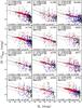 |
Fig. 2 A random realization of the Monte Carlo interloper subtraction technique. Only galaxies assigned to the clusters are shown: red dots are morphologically early-type galaxies (Es and S0s), blue dots are late-type ones and black dots are galaxies with no available morphological classification (colors only available in the on-line version). The best-fitted RS of the 100 realizations is drawn (solid black line) with ± 0.2 mag limits (dashed black lines) identifying the red sequence. The rms numerical values are reported at the top of each panel. The global properties of each cluster are reported, for reference, at the bottom of each panel. The vertical lines mark the absolute V magnitude limits used to define the luminous and the faint population of the RS. |
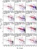 |
Fig. 2 continued. |
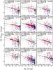 |
Fig. 2 continued. |
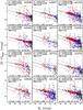 |
Fig. 2 continued. |
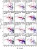 |
Fig. 2 continued. |
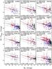 |
Fig. 2 continued. |
3.2. Defining the red sequence
We calculated rest-frame absolute magnitudes and colors by applying a galaxy-type dependent k-correction based on the observed (B − V) color of the galaxies within an aperture (diameter) of 10.8 kpc using the K-corrections from Poggianti (1997). The physical aperture assures a well-sampled, distance-independent color for all galaxies. We applied a cut in color 0.5 ≤ (B − V)10.8 kpc ≤ 1.5 to eliminate those eventual (few) galaxies that are surely either too red or too blue to belong to our clusters but might have remained after the statistical subtraction. In the following, we consider only galaxies brighter than MV ~ −18 for which both our photometric and morphological catalogs are complete (Varela et al. 2009; Fasano et al. 2011).
We used the robust bi-weight estimator fitting procedure in two steps to identify the RS. The first step consisted of fitting all the galaxies from the previous selection process with absolute V magnitude −21.5 ≤ MV ≤ −18 and calculating the median distance dred of all the galaxies from the best fit. We chose this magnitude interval because most of our CMDs (see Fig. 1) exhibit a change of slope (are shallower) at higher luminosities.
In the second step only data for galaxies with −21.5 ≤ MV ≤ −18 and distance 3 × dred from the previous step were fitted, and the rms of the residuals were calculated. Only galaxies within 0.2 mag of the second fit were assigned to the RS-population2. All non RS-galaxies bluer than that were assigned to the blue population.
This procedure was applied to each of the 100 Monte Carlo Simulations and a final mean value and its error were found for each individual cluster (see Table 1). In Fig. 2, we present a sample plot of one of the Monte Carlo realizations for each cluster, with the best-fit parameters and the global scatter in the red sequence and the main properties of the cluster shown at the bottom of each panel. The vertical lines indicate the V-band absolute magnitude limits used to define the “luminous” and the “faint” red sequence population (see Sect. 4.2).
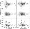 |
Fig. 3 Slope, value of best fit line at MV = −20 and scatter of the median RS values of the 100 Monte Carlo runs for each cluster versus cluster velocity dispersion (σclus, left panels) and cluster X-ray luminosity (LX, right panels). Error bars refer to the error of the median of the 100 simulations. In red (on-line version), clusters whose RS is contaminated by another structure (see text). |
4. Results
4.1. Slope and scatter
In Table 1, in addition to the global parameters of our cluster sample, we present the median slope and scatter of the 100 Monte Carlo realizations described in Sect. 3.2. The median slope for all our clusters is − 0.047 ± 0.001, and the typical scatter is of the order of ~0.05 mag.
In Fig. 3 we plot the slope, the fit value at MV = −20, and the scatter of the RS against the cluster velocity dispersion and total X-ray luminosity (both of which are related to the cluster mass). We indicate in red those clusters whose RS appears to be contaminated by another galaxy structure visible in Fig. 2 (A133, A151, A548b, A2149, A2382, A2415, A3490, A3667, and A3809)3, although it should be kept in mind that several other clusters have a very broad RS suggestive of more than one structure along the line of sight and close in redshift to the main cluster.
If the epoch and rate at which galaxies turn red and reach the color − magnitude RS depended upon the mass of the cluster to which galaxies belong at z = 0, we should observe a correlation between cluster mass and RS properties. Instead, we do not find any such correlation in our sample of 72 local clusters.
Similarly, we do not find any dependence of the RS slope, scatter, and MV = −20 value on the number of substructures, the BCG prevalence value, and the concentration of ellipticals (not shown). Our results agree with the previous findings of Stott et al. (2009), which showed a lack of correlation between the RS slope and the cluster σ, LX, and BCG dominance at z = 0.1 − 1.
4.2. Luminous-to-faint ratio and blue fractions
The number ratio of luminous-to-faint RS galaxies is often used to investigate the evolution of the faint end of the red luminosity function of cluster galaxies. High-z studies find a deficiency of faint red galaxies in comparison to local galaxy clusters, as the luminous-to-faint ratio is seen to evolve from higher values at high-z to lower values at low-z (see, among others, De Lucia et al. 2004; Tanaka et al. 2005; De Lucia et al. 2007; Stott et al. 2007; Gilbank et al. 2008; Lu et al. 2009; Rudnick et al. 2009; Stott et al. 2009; Capozzi et al. 2010; and Andreon 2008; Crawford et al. 2009 for different conclusions). This is generally interpreted as evidence of a large number of relatively faint galaxies having moved to the RS only recently, most probably due to the quenching of star formation caused by the high-density environment. The luminous-to-faint ratio has also been found to evolve in the field, but to be lower in clusters than in the field at all redshifts out to z = 1, implying that the faint end of the red sequence was established first in clusters (Gilbank & Balogh 2008).
We wish to study how the luminous-to-faint RS ratio changes from cluster to cluster and depends on cluster properties at low redshift. To define the two galaxy populations, we corrected our absolute magnitudes for passive evolution: we consider all galaxies brighter than MV = −20 − lumcorr to be luminous, and all galaxies fainter than this magnitude and brighter than MV = −18.2 − lumcorr to be faint, where lumcorr is the passive evolution correction with respect to z = 0. We recall here that these are the same absolute V magnitude limits adopted by De Lucia et al. (2007) and most other works at high redshift, but that high-z studies usually consider the (U − V) rest-frame color, hence a direct comparison cannot be performed.
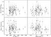 |
Fig. 4 Luminous-to-faint ratio (top panels) and blue fraction (bottom panels) versus cluster velocity dispersion and total X-ray luminosity in WINGS clusters. Errorbars are the mean error in the 100 Monte Carlo realizations. |
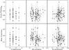 |
Fig. 5 Luminous-to-faint ratio (top panels) and blue fraction (bottom panels) versus number of substructures, BCG prevalence value and concentration of elliptical galaxies in WINGS clusters. Errorbars are the mean error in the 100 Monte Carlo realizations. |
Our large sample of local clusters show a large scatter in the luminous-to-faint ratio. In the top panels of Figs. 4 and 5, we plot the luminous-to-faint ratio as a function of cluster velocity dispersion, X-ray luminosity, number of substructures, BCG prevalence value, and concentration of ellipticals.
As for the RS parameters, no correlation between the luminous-to-faint ratio and the cluster properties was found. This agrees with the results of Capozzi et al. (2010), who found no relationship between luminous-to-faint ratio and cluster X-ray luminosity at low redshift, and with Rudnick et al. (2009), who failed to detect a dependence of the red galaxy luminosity function on cluster velocity dispersion in the SDSS.
Such a lack of a correlation suggests that the downsizing trend in star formation (i.e. how the different distribution of times at which galaxies turn red and reach the RS depends on their luminosity) does not depend in a simple way on global cluster properties such as the cluster mass, or level of substructure. However, the large scatter in the luminous-to-faint values of our sample shows that there is a great diversity in the way that the RS is populated as a function of galaxy magnitude. Most likely, this indicates widely different quenching histories in faint galaxies from cluster to cluster, even for clusters of the same mass at z = 0.
The blue fraction is defined as the ratio of the number of blue galaxies to the total number of galaxies in the cluster, for MV < −18.2. In the past decade, the blue fraction has been observed to have a large scatter in values at any given redshift, and to depend on several obvious parameters such as the magnitude limit used and the cluster-centric distance. However, often conflicting conclusions have been reached as to whether it depends on cluster properties such as concentration, richness, and the presence of substructure (Butcher & Oemler 1984; Wang & Ulmer 1997; Smail et al. 1998; Metevier et al. 2000; Ellingson et al. 2001; Margoniner et al. 2001; Pimbblet et al. 2002; Fairley et al. 2002; Balogh et al. 2004; De Propris et al. 2004; Barkhouse et al. 2009). All these findings together imply that environmental effects may compete with, and possibly mimic, evolutionary trends. Thus, it is of paramount importance to try to distinguish the cluster-to-cluster variance and the dependence on cluster properties in order to properly understand and interpret the studies of high-z clusters and investigate how the current galaxy populations in clusters came to be.
 |
Fig. 6 Morphological fractions on the RS vs. central velocity dispersion and total X-ray luminosity of the WINGS clusters. Errorbars are the mean error in the 100 Monte Carlo realizations. “Early” late-type galaxies are Sa’s and Sb’s, while “late” late-type galaxies are Sc’s and later. |
In Fig. 4 (bottom panels) we illustrate that in WINGS there is no dependence of the blue fraction on either cluster velocity dispersion or total X-ray luminosity, as found previously in the local Universe and at higher redshifts (Fairley et al. 2002; De Propris et al. 2004; Goto 2005), and in agreement with a flat median star-forming (emission-line) fraction for clusters with σ > 500 km s-1 in the local Universe (Poggianti et al. 2006; Popesso et al. 2007). Furthermore, we find no trend with the number of substructures, the BCG prevalence value and the concentration of elliptical galaxies (Fig. 5). A quite large scatter in the blue fraction is found when we fix any of these parameters, though most clusters have a blue fraction below 20%, with a median of 0.16 ± 0.03.
Poggianti et al. (2006) proposed a scenario in which the population of passive galaxies (those devoid of ongoing star formation at the time they are observed) consists of two different components: primordial passive galaxies (the most massive, mostly ellipticals) whose stars all formed at z > 2 − 3, and quenched galaxies (on average less massive, mostly S0s) whose star formation was truncated by the dense environment at later times. Comparing with simulations, they found that at z = 0 the observed fraction of passive galaxies in clusters resembles the fraction (in mass and number of galaxies) that has resided in clusters (Msys > 1014 M⊙) during at least the past 3 Gyr.
In this picture, the median fraction of star-forming galaxies, and the median blue fraction we observe, correlate with neither the cluster σ nor LX. This is because in clusters more massive than 500 km s-1 at z = 0, the median fraction of galaxies that have spent enough time in a massive environment to have their star formation quenched by some (unidentified) environmental mechanism does not vary systematically with cluster mass. This may be a viable explanation also for the lack of correlation between the luminous-to-faint ratio and the global cluster properties, as the blue galaxies and the faint red galaxies together form the overall faint cluster population subject to quenching.
4.3. Morphological fractions and red spirals
When studying the CMD and, more generally, the evolution of galaxy clusters, it is important to evaluate the fractions of the different morphological types residing on the red sequence. Indeed, apart from the well-known presence of red Es in galaxy clusters, it is not completely clear if there is some correlation between the frequency of red S0s and late-type galaxies and the global properties of the clusters. The presence of S0s and late-type galaxies on the RS is often ascribed to the capacity of the hostile cluster environment to quench star formation or even strip and/or induce a fading of the disks of galaxies of the later types.
It is apparent from Fig. 6 that there is no dependence of the RS morphological fractions on either X-ray luminosity or cluster velocity dispersion. Similarly, no correlations were found with the number of substructures, the BCG prevalence value, and the concentration of ellipticals (plot not shown). In the scenario of a double channel for passive galaxies discussed above, these results are expected given that the median fractions of both primordial (ellipticals) and quenched galaxies (S0s) are constant with cluster velocity dispersion (see Fig. 16 in Poggianti et al. 2006).
The median morphological fractions of galaxies on the RS are 0.35 ± 0.05 for ellipticals, 0.46 ± 0.04 for S0s, 0.17 ± 0.04 for early spirals (Sa to Sbc, 0 < Ttype ≤ 4) and 0.02 ± 0.02 for later type spirals (4 < T ≤ 8).
It is interesting to compare these values with those found by Sánchez-Blázquez et al. (2009) in clusters at z = 0.4 − 0.8, which were obtained adopting similar cluster radial limits and galaxy magnitude (passively evolved) limits to those in our study. These authors found an increase in the late-type fraction on the red sequence, from 25% at z = 0.75 to 44% at z = 0.45, because the red-sequence becomes more populated at later times with disc galaxies whose star formation has been quenched. Interestingly, however, the same authors predict a subsequent decrease in the red late-type fraction from z = 0.45 to z = 0, owing to the combination of the strong morphological evolution from spirals to S0s and the mild variation in the RS luminous-to-faint ratio observed in this redshift interval.
Our ~20% fraction of late-type galaxies on the RS is indeed much lower than the value observed at z = 0.45, and is consistent with a scenario in which over the interval z = 1−0.4 the RS becomes populated with spirals that have stopped forming stars, a quite large fraction of which are transformed into S0s at z < 0.4 (Desai 2007; Dressler et al. 1997; Fasano et al. 2000; Postman et al. 2005).
4.4. Elliptical to S0 ratios and cluster evolution
When considering the formation history of galaxy clusters, one may expect that clusters with a large presence of red spirals may also have a larger fraction of S0s than Es on the RS. In other words, clusters with a larger number of passive late-type galaxies could have transformed a larger number of them into S0s.
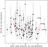 |
Fig. 7 Elliptical to S0 number ratio on the RS vs. late-type fraction on the RS. Errorbars are the mean error in the 100 Monte Carlo realizations. Red crosses and corresponding errorbars represent the mean E/S0 values and their sigma in three bins of late-type fraction. |
Figure 7 shows the relation between the RS late-type fraction and the RS ratio of Es to S0s. Clusters with a larger fraction of red spirals tend to have a population of early-type galaxies on the RS that have predominantly S0 morphologies. According to the Spearman test, the E/S0 number ratio on the RS is anticorrelated with the late-type fraction on the RS with a 95% probability.
5. The main driver: the local density
We have shown that the RS parameters, luminous-to-faint ratio, blue fraction, and morphological fractions on the RS depend on neither the cluster global properties such as velocity dispersion or X-ray luminosity, nor the elliptical galaxy concentration, BCG prevalence, or number of substructures.
In Figs. 8 and 9, we show that all the galaxy properties considered do, however, vary with the local galaxy density. Most noticeably, higher density regions have a tighter RS (smaller RS scatter), and a lower fraction of blue galaxies. The RS generally becomes steeper (RS slope increases) with local density, except for a high value in the lowest density bin. We note that a dependence of the location of both the CM relation and the blue fraction on local density has been found before in the Shapley supercluster at z = 0.05 by Haines et al. (2006).
The high value of the RS slope in the lowest density bin is accompanied by slighly larger values of both the fraction of ellipticals and the E/S0 number ratio than in denser regions (Fig. 9). It is difficult to assess the significance of these single points, and wider images will be needed to sample the lower density outer regions of clusters.
Interestingly, the RS luminous-to-faint ratio increases monotonically with local density (Fig. 8), implying that the relative proportion of luminous to faint red galaxies is higher in denser regions. This is the first time that such a trend has been observed. At high-z, the opposite trend has been found, consistent with a scenario in which the build-up of the CMR is delayed in lower density environments (Tanaka et al. 2005; Tanaka et al. 2007). The increase in the luminous-to-faint ratio with density in WINGS clusters seems to reflect, instead, the fact that higher density regions in WINGS host proportionally more high-mass than low-mass galaxies (regardless of color) than lower density regions, as shown in Vulcani et al. (2011).
Finally, higher density regions have a smaller fraction of spirals on the RS than lower density regions (Fig. 9): the RS in the highest density regions contains only a few spirals (~10%), while the RS in low density regions consists of up to 30% of spirals. The relative proportion of ellipticals and S0s does not change with local density, except for the highest density regions where ellipticals dominate.
It is important to stress that the correlations between RS properties and local density shown in Fig. 8 are not driven by differences between the RS properties of the different morphological types in combination with the morphology-density relation. In particular, we wished to test whether a larger fraction of spirals at low densities might induce the trends observed. We found that none of the conclusions from Fig. 8 change if we include only ellipticals, S0s, or ellipticals+S0s.
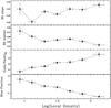 |
Fig. 8 RS slope and scatter, luminous-to-faint ratio and blue fraction vs. galaxy local density. |
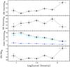 |
Fig. 9 Morphological fractions on the RS versus galaxy local density. From top to bottom: ellipticals, S0s, later-types (early-spirals and late spirals, cyan diamonds and blue squares, respectively) and E/S0 ratio. |
6. Discussion and conclusions
We have analyzed the properties of the (B − V) versus V color − magnitude RS of 72 X-ray selected clusters at z = 0.04−0.07 from the WINGS survey.
We have searched for correlations between the characteristics of the RS and the properties of both the global and local environment, finding the following main results:
The location and parameters of the RS, as well as the magnitude and morphological distributions of its galaxies, do not depend on global cluster properties. Specifically:
-
neither the slope nor the scatter of the RS; nor
-
the number ratio of luminous-to-faint galaxies on the RS; nor
-
the fraction of blue galaxies; nor
-
the morphological mix on the RS, that is, the fraction of galaxies on the RS that are ellipticals, S0s and spirals,
-
-
We have found a weak tendency for clusters whose RS is “rich” in S0 galaxies (compared to the population of ellipticals) to be also “rich” in red spirals. The populations of S0 and spirals on the RS are coupled at some level.
The strongest correlations we have found are those between the RS and the local galaxy density. The scatter and, possibly, the slope of the RS vary with local density, as do the luminous-to-faint ratio, blue galaxy fraction, and morphological mix of galaxies on the RS. The latter means that, remarkably, a clear morphology-density relation, especially for spirals, is visible even when we restrict the analysis to galaxies on the red sequence. However, the correlations between the RS properties and local density are not a consequence of the morphology-density relation (i.e. the larger fraction of spirals at lower densities), as all the trends in Fig. 8 persist even when restricting the analysis to only ellipticals, S0s, or early-type galaxies.
Local density thus appears to be the main factor governing the evolutionary rate of galaxies in these clusters. If this is the case, the lack of any correlation between the RS characteristics and the cluster mass is unsurprising, given that the distribution of local galaxy densities does not depend on cluster mass (Poggianti et al. 2010).
In the same way as the morphological mix of galaxies (of all colors) depends on local density (Dressler 1980) and not on cluster mass (Poggianti et al. 2009) in the local Universe, our present study highlights the prominent effect of the local density, in contrast to the mass of the galaxy host structure in setting the passivization epoch of galaxies and their arrival on the RS, and the subsequent morphological transformation to S0s.
The dependence of the RS properties on local density can originate from several mechanisms, and at different cosmological epochs. Since the present local density is expected to correlate with the initial density in the primordial phases, the star formation process may be accelerated in dense regions from the start, leading to shorter formation times. Physical processes acting at later times, among those commonly refered to as environmental mechanisms, can accelerate and/or quench star formation more efficiently in denser regions. Among these are gravitational interactions between galaxies, before or after the accretion of galaxies onto clusters, and gas removal mechanisms. While a detailed modeling of these processes is beyond the scope of this paper, the combination of the lack of trends with cluster mass and the observed correlations with local density represent a solid observational contraint for future studies.
Please refer to the WINGS website for updated details on the survey and its products, http://web.oapd.inaf.it/wings
Using galaxies within 2 × rms from the fit did not change any of the results of this paper.
We have not highlighted here those fields with a second RS of a cluster at sufficiently higher redshift not to influence the RS of the main WINGS structure, such as A2572, A3560, A3490, and RX1022.
Acknowledgments
We thank the anonymous referee for her/his comments that led to improvements of this paper, and Diego Capozzi for useful discussions and comments.
T. Valentinuzzi acknowledges a post-doc fellowship from the Ministero dell’Istruzione, dell’Università e della Ricerca (Italy). B.V. and B.M.P. acknowledge financial support from ASI contract I/016/07/0.
This research has made use of the NASA/IPAC Extragalactic Database (NED) which is operated by the Jet Propulsion Laboratory, California Institute of Technology, under contract with the National Aeronautics and Space Administration.
IRAF (Image Reduction and Analysis Facility) is written and supported by the IRAF programming group at the National Optical Astronomy Observatories (NOAO) in Tucson, Arizona. NOAO is operated by the Association of Universities for Research in Astronomy (AURA), Inc. under cooperative agreement with the National Science Foundation.
References
- Abraham, R. G., van den Bergh, S., & Nair, P. 2003, ApJ, 588, 218 [NASA ADS] [CrossRef] [Google Scholar]
- Andreon, S. 2008, MNRAS, 386, 1045 [NASA ADS] [CrossRef] [Google Scholar]
- Balogh, M. L., Baldry, I. K., Nichol, R., et al. 2004, ApJ, 615, L101 [NASA ADS] [CrossRef] [Google Scholar]
- Balogh, M. L., McGee, S. L., Wilman, D., et al. 2009, MNRAS, 398, 754 [NASA ADS] [CrossRef] [Google Scholar]
- Barkhouse, W. A., Yee, H. K. C., & López-Cruz, O. 2009, ApJ, 703, 2024 [NASA ADS] [CrossRef] [Google Scholar]
- Bell, E. F., Wolf, C., Meisenheimer, K., et al. 2004, ApJ, 608, 752 [NASA ADS] [CrossRef] [Google Scholar]
- Bell, E. F., Zheng, X. Z., Papovich, C., et al. 2007, ApJ, 663, 834 [NASA ADS] [CrossRef] [Google Scholar]
- Bekki, K. 2009, MNRAS, 399, 2221 [NASA ADS] [CrossRef] [Google Scholar]
- Berta, S., Rubele, S., Franceschini, A., et al. 2006, A&A, 451, 881 [NASA ADS] [CrossRef] [EDP Sciences] [Google Scholar]
- Bower, R. G., Lucey, J. R., & Ellis, R. S. 1992, MNRAS, 254, 589 [NASA ADS] [CrossRef] [Google Scholar]
- Bower, R. G., Benson, A. J., Malbon, R., et al. 2006, MNRAS, 370, 645 [NASA ADS] [CrossRef] [Google Scholar]
- Butcher, H., & Oemler, A., Jr. 1984, ApJ, 285, 426 [NASA ADS] [CrossRef] [Google Scholar]
- Capozzi, D., Collins, C. A., & Stott, J. P. 2010, MNRAS, 403, 1274 [NASA ADS] [CrossRef] [Google Scholar]
- Cava, A., Bettoni, D., Poggianti, B. M., et al. 2009, A&A, 495, 707 [NASA ADS] [CrossRef] [EDP Sciences] [Google Scholar]
- Cheng, J. Y., Faber, S. M., Simard, L., et al. 2011, MNRAS, 412, 727 [NASA ADS] [Google Scholar]
- Conselice, C. J. 2003, ApJS, 147, 1 [NASA ADS] [CrossRef] [Google Scholar]
- Conselice, C. J., Bershady, M. A., & Jangren, A. 2000, ApJ, 529, 886 [NASA ADS] [CrossRef] [Google Scholar]
- Cowie, L. L., Songaila, A., Hu, E. M., & Cohen, J. G. 1996, AJ, 112, 839 [Google Scholar]
- Crawford, S. M., Bershady, M. A., & Hoessel, J. G. 2009, ApJ, 690, 1158 [NASA ADS] [CrossRef] [Google Scholar]
- Croton, D. J., Springel, V., White, S. D. M., et al. 2006, MNRAS, 365, 11 [NASA ADS] [CrossRef] [Google Scholar]
- Dariush, A. A., Raychaudhury, S., Ponman, T. J., et al. 2010, MNRAS, 405, 1873 [NASA ADS] [Google Scholar]
- De Lucia, G., Poggianti, B. M., Aragón-Salamanca, A., et al. 2004, ApJ, 610, L77 [NASA ADS] [CrossRef] [Google Scholar]
- De Lucia, G., Poggianti, B. M., Aragón-Salamanca, A., et al. 2007, MNRAS, 374, 809 [NASA ADS] [CrossRef] [Google Scholar]
- De Propris, R., Colless, M., Peacock, J. A., et al. 2004, MNRAS, 351, 125 [NASA ADS] [CrossRef] [Google Scholar]
- Desai, V., Dalcanton, J. J., Aragón-Salamanca, A., et al. 2007, ApJ, 660, 1151 [NASA ADS] [CrossRef] [Google Scholar]
- de Vaucouleurs, G. 1961, ApJS, 5, 233 [NASA ADS] [CrossRef] [Google Scholar]
- Dressler, A. 1980, ApJ, 236, 351 [NASA ADS] [CrossRef] [Google Scholar]
- Dressler, A., Oemler, A., Couch, W. J., et al. 1997, ApJ, 490, 577 [NASA ADS] [CrossRef] [Google Scholar]
- Ebeling, H., Voges, W., Bohringer, H., et al. 1996, MNRAS, 281, 799 [NASA ADS] [CrossRef] [Google Scholar]
- Ebeling, H., Edge, A. C., Bohringer, H., et al. 1998, MNRAS, 301, 881 [NASA ADS] [CrossRef] [Google Scholar]
- Ebeling, H., Edge, A. C., Allen, S. W., et al. 2000, MNRAS, 318, 333 [NASA ADS] [CrossRef] [Google Scholar]
- Ellingson, E., Lin, H., Yee, H. K. C., & Carlberg, R. G. 2001, ApJ, 547, 609 [NASA ADS] [CrossRef] [Google Scholar]
- Ellis, R. S., Smail, I., Dressler, A., et al. 1997, ApJ, 483, 582 [NASA ADS] [CrossRef] [Google Scholar]
- Faber, S. M., Willmer, C. N. A., Wolf, C., et al. 2007, ApJ, 665, 265 [NASA ADS] [CrossRef] [Google Scholar]
- Fairley, B. W., Jones, L. R., Wake, D. A., et al. 2002, MNRAS, 330, 755 [NASA ADS] [CrossRef] [Google Scholar]
- Fasano, G., Poggianti, B. M., Couch, W. J., et al. 2000, ApJ, 542, 673 [NASA ADS] [CrossRef] [Google Scholar]
- Fasano, G., Marmo, C., Varela, J., et al. 2006, A&A, 445, 805 [NASA ADS] [CrossRef] [EDP Sciences] [Google Scholar]
- Fasano, G., Bettoni, D., Ascaso, B., et al. 2010, MNRAS, 404, 1490 [NASA ADS] [Google Scholar]
- Fasano, G., Vanzella, E., Dressler, A., et al. 2011, MNRAS, accepted [arXiv:1109.2026] [Google Scholar]
- Font, A. S., Bower, R. G., McCarthy, I. G., et al. 2008, MNRAS, 389, 1619 [NASA ADS] [CrossRef] [Google Scholar]
- Gilbank, D. G., & Balogh, M. L. 2008, MNRAS, 385, L116 [NASA ADS] [CrossRef] [Google Scholar]
- Gilbank, D. G., Yee, H. K. C., Ellingson, E., et al. 2008, ApJ, 673, 742 [NASA ADS] [CrossRef] [Google Scholar]
- Gilbank, D. G., Gladders, M. D., Yee, H. K. C., & Hsieh, B. C. 2011, AJ, 141, 94 [NASA ADS] [CrossRef] [Google Scholar]
- Gladders, M. D., & Yee, H. K. C. 2005, ApJS, 157, 1 [NASA ADS] [CrossRef] [Google Scholar]
- Goto, T. 2005, MNRAS, 356, L6 [NASA ADS] [CrossRef] [Google Scholar]
- Gunn, J. E., & Gott, J. R., III 1972, ApJ, 176, 1 [NASA ADS] [CrossRef] [Google Scholar]
- Guo, Q., White, S., Boylan-Kolchin, M., et al. 2011, MNRAS, 413, 101 [NASA ADS] [CrossRef] [Google Scholar]
- Haines, C. P., Merluzzi, P., Mercurio, A., et al. 2006, MNRAS, 371, 55 [NASA ADS] [CrossRef] [Google Scholar]
- Kauffmann, G., Heckman, T. M., White, S. D. M., et al. 2003, MNRAS, 341, 54 [Google Scholar]
- Kimm, T., Somerville, R. S., Yi, S. K., et al. 2009, MNRAS, 394, 1131 [NASA ADS] [CrossRef] [Google Scholar]
- Kodama, T., & Bower, R. G. 2001, MNRAS, 321, 18 [NASA ADS] [CrossRef] [Google Scholar]
- Kodama, T., Arimoto, N., Barger, A. J., & Arag’on-Salamanca, A. 1998, A&A, 334, 99 [NASA ADS] [Google Scholar]
- Lidman, C., Rosati, P., Tanaka, M., et al. 2008, A&A, 489, 981 [NASA ADS] [CrossRef] [EDP Sciences] [Google Scholar]
- Loh, Y.-S., Ellingson, E., Yee, H. K. C., et al. 2008, ApJ, 680, 214 [NASA ADS] [CrossRef] [Google Scholar]
- Lotz, J. M., Primack, J., & Madau, P. 2004, AJ, 128, 163 [NASA ADS] [CrossRef] [Google Scholar]
- Lu, T., Gilbank, D. G., Balogh, M. L., & Bognat, A. 2009, MNRAS, 399, 1858 [NASA ADS] [CrossRef] [Google Scholar]
- Margoniner, V. E., de Carvalho, R. R., Gal, R. R., & Djorgovski, S. G. 2001, ApJ, 548, L143 [NASA ADS] [CrossRef] [Google Scholar]
- McCarthy, I. G., Schaye, J., Ponman, T. J., et al. 2010, MNRAS, 406, 822 [NASA ADS] [Google Scholar]
- Mei, S., Holden, B. P., Blakeslee, J. P., et al. 2009, ApJ, 690, 42 [NASA ADS] [CrossRef] [Google Scholar]
- Metevier, A. J., Romer, A. K., & Ulmer, M. P. 2000, AJ, 119, 1090 [NASA ADS] [CrossRef] [Google Scholar]
- Moore, B., Lake, G., & Katz, N. 1998, ApJ, 495, 139 [NASA ADS] [CrossRef] [Google Scholar]
- Muzzin, A., Wilson, G., Yee, H. K. C., et al. 2009, ApJ, 698, 1934 [NASA ADS] [CrossRef] [Google Scholar]
- Peng, Y., Lilly, S. J., Kovac, K., et al. 2010, ApJ, 721, 193 [NASA ADS] [CrossRef] [Google Scholar]
- Pimbblet, K. A., Smail, I., Kodama, T., et al. 2002, MNRAS, 331, 333 [NASA ADS] [CrossRef] [Google Scholar]
- Poggianti, B. M. 1997, A&AS, 122, 399 [NASA ADS] [CrossRef] [EDP Sciences] [Google Scholar]
- Poggianti, B. M., von der Linden, A., De Lucia, G., et al. 2006, ApJ, 642, 188 [NASA ADS] [CrossRef] [Google Scholar]
- Poggianti, B. M., Fasano, G., Bettoni, D., et al. 2009, ApJ, 697, L137 [NASA ADS] [CrossRef] [Google Scholar]
- Poggianti, B. M., De Lucia, G., Varela, J., et al. 2010, MNRAS, 405, 995 [NASA ADS] [Google Scholar]
- Popesso, P., Biviano, A., Romaniello, M., & Böhringer, H. 2007, A&A, 461, 411 [NASA ADS] [CrossRef] [EDP Sciences] [Google Scholar]
- Postman, M., Franx, M., Cross, N. J. G., et al. 2005, ApJ, 623, 721 [NASA ADS] [CrossRef] [Google Scholar]
- Ramella, M., Biviano, A., Pisani, A., et al. 2007, A&A, 470, 39 [NASA ADS] [CrossRef] [EDP Sciences] [Google Scholar]
- Rudnick, G., von der Linden, A., Pelló, R., et al. 2009, ApJ, 700, 1559 [NASA ADS] [CrossRef] [Google Scholar]
- Sánchez-Blázquez, P., Jablonka, P., Noll, S., et al. 2009, A&A, 499, 47 [NASA ADS] [CrossRef] [EDP Sciences] [Google Scholar]
- Smail, I., Edge, A. C., Ellis, R. S., & Blandford, R. D. 1998, MNRAS, 293, 124 [NASA ADS] [CrossRef] [Google Scholar]
- Stott, J. P., Smail, I., Edge, A. C., et al. 2007, ApJ, 661, 95 [NASA ADS] [CrossRef] [Google Scholar]
- Stott, J. P., Pimbblet, K. A., Edge, A. C., Smith, G. P., & Wardlow, J. L. 2009, MNRAS, 394, 2098 [NASA ADS] [CrossRef] [Google Scholar]
- Strateva, I., Ivezić, Z., Knapp, G. R., et al. 2001, AJ, 122, 1861 [Google Scholar]
- Strazzullo, V., Rosati, P., Pannella, M., et al. 2010, A&A, 524, A17 [NASA ADS] [CrossRef] [EDP Sciences] [Google Scholar]
- Tanaka, M., Kodama, T., Arimoto, N., et al. 2005, MNRAS, 362, 268 [NASA ADS] [CrossRef] [Google Scholar]
- Tanaka, M., Kodama, T., Kajisawa, M., et al. 2007, MNRAS, 377, 1206 [NASA ADS] [CrossRef] [Google Scholar]
- Valentinuzzi, T., Woods, D., Fasano, G., et al. 2009, A&A, 501, 851 [NASA ADS] [CrossRef] [EDP Sciences] [Google Scholar]
- van den Bosch, F. C., Aquino, D., Yang, X., et al. 2008, MNRAS, 387, 79 [Google Scholar]
- Varela, J., D’Onofrio, M., Marmo, C., et al. 2009, A&A, 497, 667 [NASA ADS] [CrossRef] [EDP Sciences] [Google Scholar]
- Visvanathan, N., & Sandage, A. 1977, ApJ, 216, 214 [NASA ADS] [CrossRef] [Google Scholar]
- Wang, Q. D., & Ulmer, M. P. 1997, MNRAS, 292, 920 [NASA ADS] [CrossRef] [Google Scholar]
- Wilson, G., Muzzin, A., Yee, H. K. C., et al. 2009, ApJ, 698, 1943 [NASA ADS] [CrossRef] [Google Scholar]
All Tables
All Figures
|
Fig. 1 Visual example of a Monte Carlo realization for the cluster Abell 119. In the upper panel, the red empty dots and the black filled dots are the non-members and members assigned by the simulation (run 37th), respectively. Shown as green circles and blue crosses are the spectroscopic members and non-members, respectively. In the middle panel, only members according to the Monte Carlo realization are shown, but divided into different morphological types (see legend and the figure in electronic format). In the bottom panel, the RS extracted is shown, again with the morphological color coding. The dotted vertical lines mark the absolute V magnitude limits used to define the luminous and faint population on the RS. |
| In the text | |
|
Fig. 2 A random realization of the Monte Carlo interloper subtraction technique. Only galaxies assigned to the clusters are shown: red dots are morphologically early-type galaxies (Es and S0s), blue dots are late-type ones and black dots are galaxies with no available morphological classification (colors only available in the on-line version). The best-fitted RS of the 100 realizations is drawn (solid black line) with ± 0.2 mag limits (dashed black lines) identifying the red sequence. The rms numerical values are reported at the top of each panel. The global properties of each cluster are reported, for reference, at the bottom of each panel. The vertical lines mark the absolute V magnitude limits used to define the luminous and the faint population of the RS. |
| In the text | |
|
Fig. 2 continued. |
| In the text | |
|
Fig. 2 continued. |
| In the text | |
|
Fig. 2 continued. |
| In the text | |
|
Fig. 2 continued. |
| In the text | |
|
Fig. 2 continued. |
| In the text | |
|
Fig. 3 Slope, value of best fit line at MV = −20 and scatter of the median RS values of the 100 Monte Carlo runs for each cluster versus cluster velocity dispersion (σclus, left panels) and cluster X-ray luminosity (LX, right panels). Error bars refer to the error of the median of the 100 simulations. In red (on-line version), clusters whose RS is contaminated by another structure (see text). |
| In the text | |
|
Fig. 4 Luminous-to-faint ratio (top panels) and blue fraction (bottom panels) versus cluster velocity dispersion and total X-ray luminosity in WINGS clusters. Errorbars are the mean error in the 100 Monte Carlo realizations. |
| In the text | |
|
Fig. 5 Luminous-to-faint ratio (top panels) and blue fraction (bottom panels) versus number of substructures, BCG prevalence value and concentration of elliptical galaxies in WINGS clusters. Errorbars are the mean error in the 100 Monte Carlo realizations. |
| In the text | |
|
Fig. 6 Morphological fractions on the RS vs. central velocity dispersion and total X-ray luminosity of the WINGS clusters. Errorbars are the mean error in the 100 Monte Carlo realizations. “Early” late-type galaxies are Sa’s and Sb’s, while “late” late-type galaxies are Sc’s and later. |
| In the text | |
|
Fig. 7 Elliptical to S0 number ratio on the RS vs. late-type fraction on the RS. Errorbars are the mean error in the 100 Monte Carlo realizations. Red crosses and corresponding errorbars represent the mean E/S0 values and their sigma in three bins of late-type fraction. |
| In the text | |
|
Fig. 8 RS slope and scatter, luminous-to-faint ratio and blue fraction vs. galaxy local density. |
| In the text | |
|
Fig. 9 Morphological fractions on the RS versus galaxy local density. From top to bottom: ellipticals, S0s, later-types (early-spirals and late spirals, cyan diamonds and blue squares, respectively) and E/S0 ratio. |
| In the text | |
Current usage metrics show cumulative count of Article Views (full-text article views including HTML views, PDF and ePub downloads, according to the available data) and Abstracts Views on Vision4Press platform.
Data correspond to usage on the plateform after 2015. The current usage metrics is available 48-96 hours after online publication and is updated daily on week days.
Initial download of the metrics may take a while.