| Issue |
A&A
Volume 670, February 2023
|
|
|---|---|---|
| Article Number | A17 | |
| Number of page(s) | 16 | |
| Section | Cosmology (including clusters of galaxies) | |
| DOI | https://doi.org/10.1051/0004-6361/202244626 | |
| Published online | 30 January 2023 | |
Structural and dynamical modeling of WINGS clusters
III. The pseudo phase-space density profile
1
INAF-Osservatorio Astronomico di Trieste, Via G. B. Tiepolo 11, 34143 Trieste, Italy
e-mail: andrea.biviano@inaf.it
2
IFPU-Institute for Fundamental Physics of the Universe, Via Beirut 2, 34014 Trieste, Italy
3
Institut d’Astrophysique de Paris, UMR 7095: CNRS & Sorbonne Université, 98 bis Bd Arago, 75014 Paris, France
Received:
29
July
2022
Accepted:
28
November
2022
Numerical simulations indicate that cosmological halos display power-law radial profiles of pseudo phase-space density (PPSD), Q ≡ ρ/σ3, where ρ is the mass density and σ is the velocity dispersion. We tested these predictions for Q(r) using the parameters derived from the Markov chain Monte Carlo (MCMC) analysis performed with the MAMPOSSt mass-orbit modeling code on the observed kinematics of a velocity dispersion based stack (σv) of 54 nearby regular clusters of galaxies from the WINGS data set. In the definition of PPSD, the density is either in total mass ρ (Qρ) or in galaxy number density ν (Qν) of three morphological classes of galaxies (ellipticals, lenticulars, and spirals), while the velocity dispersion (obtained by inversion of the Jeans equation using the MCMC parameters) is either the total (Qρ and Qν) or its radial component (Qr, ρ and Qr, ν). We find that the PPSD profiles are indeed power-law relations for nearly all MCMC parameters. The logarithmic slopes of our observed Qρ(r) and Qr, ρ(r) for ellipticals and spirals are in excellent agreement with the predictions for particles in simulations, but slightly shallower for S0s. For Qν(r) and Qr, ν(r), only the ellipticals have a PPSD slope matching that of particles in simulations, while the slope for spirals is much shallower, similar to that of subhalos. However, for cluster stacks based on the richness or gas temperature, the fraction of power-law PPSDs is lower (esp. Qν) and the Qρ slopes are shallower, except for S0s. The observed PPSD profiles, defined using ρ rather than ν, appear to be a fundamental property of galaxy clusters. They would be imprinted during an early phase of violent relaxation for dark matter and ellipticals, and later for spirals as they move toward dynamical equilibrium in the cluster gravitational potential, while S0s are either intermediate (richness and temperature-based stacks) or a mixed class (σv stack).
Key words: galaxies: clusters: general / galaxies: kinematics and dynamics / dark matter
© The Authors 2023
 Open Access article, published by EDP Sciences, under the terms of the Creative Commons Attribution License (https://creativecommons.org/licenses/by/4.0), which permits unrestricted use, distribution, and reproduction in any medium, provided the original work is properly cited.
This article is published in open access under the Subscribe-to-Open model. Subscribe to A&A to support open access publication.
1. Introduction
Cosmological dissipationless simulations have led to the building blocks of the standard model of dark matter, in particular through the establishment of the universality of cosmic structure (halo) density profiles, which are well characterized by the NFW (Navarro et al. 1996) and Einasto models (Navarro et al. 2004)1. Further insight into the structure of clusters of galaxies have come from the analysis of Taylor & Navarro (2001), who examined the coarse-grained phase-space density profiles of cold dark matter (DM) halos from cosmological simulations. They defined the pseudo-phase space density (PPSD) profile Q(r)≡ρ(r)/σ(r)3, where ρ(r) and σ(r) are the radial profiles of total mass density and velocity dispersion, respectively. They found Q(r) to follow a power-law Q(r)∝rα with α ≈ −1.875 over two and a half decades in radius. The equivalent PPSD built with the radial component of the velocity dispersion σr, that is Qr(r)≡ρ(r)/σr(r)3, was also found to obey a power-law relation with radial coordinate r, with a slightly steeper slope than Q(r) (Rasia et al. 2004; Dehnen & McLaughlin 2005)2. These power-law behaviors are remarkable given that the logarithmic density profile log ρ(r) and the logarithmic velocity dispersion profiles log σ(r) (total) and log σr(r) (radial) are all convex functions of log r. The slope of Q(r) matches the slope of −15/8 expected from secondary infall models based on the (quasi)-power law density profile ρ ∼ r−9/4 (Gott 1975; Gunn 1977; Bertschinger 1985), despite the fact that DM halos in the cosmological simulations of Taylor & Navarro (2001) assemble in a different way from the regular phase-space stratification process described by Gott (1975), Gunn (1977), and Bertschinger (1985).
Much effort has been employed in trying to understand why Q(r) is a simple power law, and why its slope is so close to the value predicted by the secondary infall model of Bertschinger (1985). Analytical and numerical studies have shown that the final shape of Q(r) does not depend on whether the halo evolves through major mergers or spherical infall (Manrique et al. 2003; Ascasibar et al. 2004; Austin et al. 2005; Hoffman et al. 2007). The final Q(r) configuration of cosmological halos appears to be reached very early on, that is to say soon or immediately after the early violent relaxation phase (Lynden-Bell 1967; Vass et al. 2009; Colombi 2021). Other collective relaxation processes might be important as well in shaping Q(r), such as Landau damping and radial orbit instability (Henriksen 2006; MacMillan et al. 2006). At large radii, where relaxation is still incomplete, a deviation from the power-law behavior was expected theoretically (Bertschinger 1985; Lapi & Cavaliere 2011), and also detected in numerical simulations. However, deviations from the power-law behavior never exceed 20% within the halo virial radius (Ascasibar & Gottlöber 2008; Navarro et al. 2010; Ludlow et al. 2010; Marini et al. 2021). Close to the halo center, where baryonic effects can be important, both a steepening (Lapi & Cavaliere 2011) and a flattening (Butsky et al. 2016) of Q(r) have been predicted.
Vass et al. (2009) suggested that the original physical association of Q(r) with the halo coarse phase-space density is not justified since the two quantities have different behaviors (but see Ma & He 2009). Interpretation of Q(r) in terms of the power −3/2 of the dynamical entropy of a gravitating system might prove more useful to understand its origin. Faltenbacher et al. (2007) noted the similarity in the so-defined dynamical entropy of DM particles and the thermodynamic entropy of the intra-cluster gas, outside the core of simulated clusters. He & Kang (2010) argued that Q(r) corresponds to a minimum entropy state, that is the end result of long-range (e.g., violent) relaxation processes in gravitating systems, while the state of maximum entropy is only reached locally, where short-range (e.g., two-body) relaxations dominate.
The analysis of simulations has led to contradicting conclusions on the universality of Q(r) slopes. Schmidt et al. (2008) argued that Q(r) is not universal, while Dehnen & McLaughlin (2005), Navarro et al. (2010), and Marini et al. (2021) found very similar slopes for the Q(r) of different halos (with a difference of ≲ 15%). The Q(r) slope is only mildly dependent (≈ ± 10%) on redshift (Lapi & Cavaliere 2009; Marini et al. 2021) and on the power spectrum of primordial density fluctuations (Knollmann et al. 2008; Brown et al. 2020).
Almost all numerical investigations so far have been focused on the Q(r) traced by DM particles, and similar results for Q(r) have been obtained in DM-only and hydrodynamical simulations (compare, e.g., Dehnen & McLaughlin 2005; Rasia et al. 2004). Only recently have different tracers been considered in the definition of Q(r) in the study of Marini et al. (2021), and the Q(r) slope has been found to be strongly dependent on the chosen tracer, with it being steeper for stars and shallower for galaxies (subhalos in hydrodynamical simulations) than for DM particles (α = −3, −1.3, and −1.8, respectively). This dependence is very relevant when comparing simulation-based predictions with observations since Q(r) is not an observable; ρ(r) can be inferred from stellar and galaxy kinematics, from gravitational lensing, or from the temperature and pressure of the intra-cluster gas (see, e.g., Pratt et al. 2019, for a review), but σ(r) can only be determined for the tracer of the gravitational potential. Since only the tracer σ(r) can be determined observationally, for consistency some authors have used the number density profile of the tracers, ν(r), rather than the total mass density profile ρ(r) in the definition of Q(r).
Several observational studies have confirmed the expected simulation-based power-law behavior of Q(r), both for galaxies and for clusters of galaxies. Chae (2014) found that Q(r) is a power law for Coma cluster elliptical galaxies with a slope of 1.93 ± 0.06. On larger scales, Q(r) has been measured in several clusters of galaxies over the redshift range 0.06–1.34, and it has always been found to be similar to, or at least consistent with, the simulation-based expectations, both when Q(r) was defined using the total mass density profile ρ(r) (Biviano et al. 2013, 2016, 2021; Munari et al. 2014) and when the tracer ν(r) was used instead for tracers of different colors and luminosities (Munari et al. 2015; Aguerri et al. 2017; Capasso et al. 2019).
Despite the good agreement of the simulation-based predictions with observations, the power-law behavior, and even the physical reality of Q(r) have been questioned. Nadler et al. (2017) argue against a power-law behavior of Q(r) at any radial scale and that the agreement between Q(r) found in numerical simulations and the solution of the secondary infall model of Bertschinger (1985) is purely coincidental. According to Schmidt et al. (2008), different halos follow  relations, with different best-fit values of ϵ and α, that is, ϵ = 3 is not a universal value. Arora & Williams (2020) argue that the power-law behavior of Q(r) does not have a physical origin, but it is fortuitous, as it is a consequence of the linear relation between the logarithmic slope of the mass density profile, γ ≡ dlnρ/dlnr, and the velocity anisotropy profile
  , where σθ and σr are the tangential and radial component of the velocity dispersion tensor. The linear β − γ relation was discovered by Hansen & Moore (2006) and Hansen & Stadel (2006) in a variety of simulated gravitating systems, issued from controlled simulations of halo-halo collisions and radial infall, as well as from cosmological simulations. However, the physical origin of the linear β − γ relation is not better elucidated than that of the Q(r) power law, and the relation is not clearly established in real clusters (Biviano et al. 2013, 2021; Munari et al. 2014; Aguerri et al. 2017).
Lacking a clear understanding of the physical origin(s) of either Q(r)∝rα or the linear β − γ relation, several studies have tried to investigate their consistency in the context of the dynamical equilibrium of a spherical gravitating system, as described by the Jeans equation, which for a spherical stationary system is (Binney 1980)
By assuming a linear β − γ relation, Dehnen & McLaughlin (2005) found a critical solution that satisfies  , with the value of α being dependent on only ϵ and β0, and independent of the slope of the β − γ relation. In particular, ϵ = 3 and β0 = 0 lead to α = 1.94, which is essentially the same value found in numerical simulations. Barnes et al. (2007) considered density profiles of the NFW or Einasto form, but they could not find consistent solutions of the Jeans equation with a power-law Q(r) and a linear β − γ relation similar to the relations found in simulations. They suggested that the β − γ relation for any single halo is not strictly linear, and that the β − γ relation is not just a manifestation of a scale-free Q(r). Zait et al. (2008) started from the power-law behavior of Q(r) to show that a linear β − γ relation is inconsistent with generalized NFW density profiles (Zhao 1996), but consistent with Einasto profiles of index n = 6 (see, e.g., Eq. (16) of Mamon et al. 2019, Paper II hereafter).
The behavior of Q(r) should depend on the choice of tracer used to measure σ(r) and σr(r), and possibly the density profile, when the number density profile, ν(r), is used in the definition of Q(r). However, the influence of the tracer choice on Q(r) has not been addressed yet.
In this article, we investigate Q(r) and Qr(r) in 54 nearby clusters of galaxies (0.04 < z < 0.07) from the WINGS data set (Fasano et al. 2006), which Cava et al. (2017, hereafter Paper I) found to be regular systems. In a forthcoming article (Mamon & Biviano, in prep.), we will investigate the β − γ relation in a similar fashion. We exploit the results of the kinematic analysis of Paper II, which determined the mass density and velocity anisotropy profiles, ρ(r) and β(r), of stack samples of these clusters, as well as the number density profiles for each of three morphological classes of galaxies, from Gaussian priors obtained from previous fits in Paper I of model plus the constant background of the photometric data for the same stacked clusters. For the first time, we determine Q(r) and Qr(r) separately for three different morphological classes of cluster galaxies.
In the rest of this paper, we use Q and Qr to refer to the pseudo-phase-space density profiles generically without a distinction being made as to whether they have been derived using ρ(r) or ν(r). When needed, we use subscripts to distinguish the different profiles, Qρ, Qr, ρ and Qν, Qr, ν.
The structure of this paper is the following. In Sect. 2 we describe our data set, and our method of analysis is provided in Sect. 3. In Sect. 4 we present our results. We discuss our results in Sect. 5. Section 6 provides a summary and our conclusions. Throughout this paper we adopt the following cosmological parameters: Ωm = 0.3, ΩΛ = 0.7, and H0 = 70 km s−1 Mpc−1.
2. The data set
Our analysis is based on the WINGS data set, which contains X-ray-selected clusters at 0.04 < z < 0.07 (Fasano et al. 2006) with spectroscopic coverage for cluster galaxies with a median stellar mass of log(M⋆/M⊙) = 10.0 for ellipticals (E) and 10.4 for spirals (S; Cava et al. 2009; Moretti et al. 2014; Paper II). Morphological types were derived by Fasano et al. (2006) using the MORPHOT tool. In Paper I, we defined three intervals in the MORPHOT classification parameter corresponding to the three morphological classes of ellipticals, lenticulars (S0), and spirals.
In Paper I, we identified cluster members using the Clean algorithm (Mamon et al. 2013) and selected a subsample of 68 clusters with at least 30 spectroscopic members. Using the substructure test of Dressler & Shectman (1988), we identified 54 regular and 14 irregular clusters. We then estimated r200 and v200 of these 68 clusters in three different ways: based on (i) the cluster velocity dispersion (sigv), (ii) an estimate of the cluster richness (num, Mamon et al., in prep., see Old et al. 2014), and (iii) the cluster X-ray temperature (tempX, only available for 38 of these clusters). Using these three estimates of r200, v200 in Paper I, we then stacked the 54 (38, in the case of tempX scaling) regular clusters into three pseudo-clusters, by rescaling the projected radii and rest-frame velocities of cluster galaxies by their cluster r200 and v200, respectively. These three pseudo-clusters formed the data set for the kinematic modeling that we performed in Paper II, using the MAMPOSSt algorithm of Mamon et al. (2013). Irregular clusters were not considered because MAMPOSSt is based on the Jeans equation, which being derived from the collisionless Boltzmann equation, assumes that the tracers are test particles orbiting the gravitational potential and not interacting with one another in contrast to galaxies within a substructure of an irregular cluster.
MAMPOSSt fits parametric models to the distributions of galaxies in projected phase space (projected distance to the center and line of sight velocity). The parameters are those describing the total mass density profile, ρ(r), the tracer density profiles for the three morphological types (i), νi(r), and the velocity anisotropy profiles for the three types, βi(r). MAMPOSSt speeds up the calculations by a large factor by assuming that the three spherical-coordinate components of the local velocity distribution function are Gaussian. The recovered radial profiles of mass density and velocity anisotropy are as good with MAMPOSSt as with other methods (Read et al. 2021), even though MAMPOSSt is much faster.
Here we use the results of the kinematic modeling of Paper II. More specifically, we consider the M(r) and β(r) model parameters of the outputs (chain elements) of the Markov chain Monte Carlo (MCMC) investigation of parameter space used by MAMPOSSt, using CosmoMC (Lewis et al. 2002), based on the Metropolis-Hastings algorithm. This allows us to determine Q(r) and Qr(r) at several values of r, and for the three different morphological classes, as detailed in Sect. 3. For Qν and Qr, ν, we also used the tracer number density profiles, νi(r), for each morphological class, obtained from fitting NFW models plus constant background to the photometric data and then refined in the MCMC analysis with MAMPOSSt.
For each model, MAMPOSSt was run using six MCMC parallel chains, each with over 105 elements, for a total of over 500 000 chain elements (i.e., points in parameter space) per model. We discard the 20% of the first elements of each chain of each model, which corresponds to the “burn-in” phase where the MCMC has not yet settled to its equilibrium and estimate Q(r) and Qr(r) for all remaining chains.
We consider all three stacks obtained using the three scalings, sigv, num, tempX. We present the results for the sigv scaling in the main text and discuss them in Sect. 5.1. Results for the num and tempX scalings are presented in Appendix A and discussed in Sect. 5.2 in comparison with the results obtained for the sigv scaling.
3. Analysis
The parameter values in each MCMC are used to directly derive the radial profile ν(r),ρ(r), and β(r). To determine Q(r) and Qr(r), we also derive σ(r) and σr(r) via:
![$$ \begin{aligned} \sigma _r^2(r) = \frac{1}{\nu (r)} \, \int _r^\infty \exp \left[ 2 \, \int _r^s \beta (t) \frac{\mathrm{d} t}{t} \right] \, \nu (s) \frac{G M(s)}{s^2} \, \mathrm{d} s, \end{aligned} $$](/articles/aa/full_html/2023/02/aa44626-22/aa44626-22-eq5.gif)
(van der Marel 1994; Mamon & Łokas 2005) and
![$$ \begin{aligned} \sigma ^2(r) = \left[3- 2 \, \beta (r) \right]\, \sigma _r^2(r), \end{aligned} $$](/articles/aa/full_html/2023/02/aa44626-22/aa44626-22-eq6.gif)
where M(r) is the total mass profile.
Paper II considered 30 sets of priors according to chosen models for the mass density profile:

with mass density logarithmic slope
where x = r/rs, while γ0 and γ∞ are the logarithmic slopes of the density profile at r = 0 and at infinity, respectively. The models considered in Paper II nearly all assumed γ∞ = −3, γ0 = −1 for NFW and γ0 ≠ −1 for generalized NFW (‘gNFW’), scale radius rs related to the radius where γ = −2: r−2 = (2 + γ0) rs.
We had also adopted Einasto (1965) mass models, which fit even better the distribution of radii in halos in ΛCDM dissipationless cosmological simulations (Navarro et al. 2004),
![$$ \begin{aligned} \rho (r) \propto \exp \left[-2\,n\,\left({r\over r_{-2}}\right)^{1/n}\right], \end{aligned} $$](/articles/aa/full_html/2023/02/aa44626-22/aa44626-22-eq9.gif)
yielding
The mass density models are normalized by the mass at radius r200 = c200 r−2 where the mean mass density is equal to 200 times the critical density of the Universe at z = 0.055, the median redshift of the WINGS clusters.
The anisotropy models considered in Paper II followed
where β0 and β∞ are the values of β at r = 0 and at infinity, respectively, rβ is the anisotropy radius where β is midway beween β0 and β∞, and δ is the anisotropy sharpness, with δ = 1 for Tiret et al. (2007) anisotropy and δ = 2 for the generalized Osipkov-Merritt (‘gOM’) anisotropy (Osipkov 1979; Merritt 1985). For δ = 1 or 2, the exponential term in Eq. (2) is (Appendix B of Mamon et al. 2013 for these anisotropy models and a few others)
The anisotropy radius was either a free parameter or fixed to the scale radius of the given morphology, rν, previously fitted to the photometric data in Paper I, using a projected NFW model plus a constant field surface density. In Paper II, we found that the elliptical galaxy distribution traces the mass very well, the S0 distribution traces it reasonably well, while the spiral galaxy distribution traces it very poorly. In other words, rν, E ≃ r−2, while rν, S ≃ 4 r−2.
In the present paper, among the 30 models of Paper II, we only considered single-component mass models with free inner and outer anisotropy for all three morphological types. We also excluded the models with Tiret anisotropy with anisotropy radius fixed to rβ = rν, which lead to linear β − γ relations if tracer follows mass (Mamon & Biviano, in prep.). This left us with models 6, 7, 12, and 15 in Table 2 of Paper II. Our results are therefore independent from the linear β − γ relation assumption that according to some authors could explain the power-law behavior of Q(r) and Qr(r) (Dehnen & McLaughlin 2005; Arora & Williams 2020).
All four considered Paper II models assume NFW ν(r), with a scale radius rν as a free parameter, one rν parameter for each morphological class. In models 6 and 7, ρ(r) is modeled by the gNFW profile, with γ∞ = −3 and γ0 as a free parameter (Eq. (4)). In models 12 and 15, ρ(r) is instead modeled by the NFW profile. In all four models r200, and therefore M200, is a free parameter of ρ(r), while c200 is related to M200 through the relation of Dutton & Macciò (2014):
with a Gaussian prior σ(log c200) = 0.13. Therefore the mass density profile involves 2 (NFW and n = 6 Einasto) or 3 (gNFW) free parameters.
Models 7 and 12 adopt the Tiret model for β(r), while models 6 and 15 adopt the gOM anisotropy model. Both the Tiret and the gOM models are characterized by two free parameters per each morphological class, the inner and outer velocity anisotropies β0 and β∞. The anisotropy scale radius rβ is a free parameter in Tiret models 7 and 12, whereas it is tied to the tracer scale radius, rβ = rν in gOM models 6 and 15. Thus, the anisotropy profile involves 2 (fixed rβ) to 3 (free rβ) parameters per morphological type, hence 6 (fixed rβ) to 9 (free rβ) free parameters after summing over the three morphological types.
In addition to the four models described above we consider the three following models. Model 7c is the same as model 7 but with c200 as a fully free parameter (with a uniform prior for log c from 0 to 1). Model 12e and 15e are the same as, respectively, model 12 and 15, but with a n = 6 Einasto ρ(r) in lieu of NFW. The properties of these seven models are summarized in Table 1.
Mass–velocity anisotropy models.
For each MCMC chain element, we determine Q(r) and Qr(r) at six logarithmically spaced radii, from r/r−2 = 0.125 to 4, in steps of a factor 2: r/r−2 = 2i − 4, i = 1, …, 6, that is from roughly 0.03 to 1 virial radius. We fit straight lines to the six values of log Q versus log r, log Qr versus log r, for each individual MCMC, yielding log Q(r) = a + b log(r/r−2). We measure the linearity of Q(r) and Qr(r) using the quantity l = 1 − D/L, where L is the length of the fitted line,

where xi = log(ri/r−2), and D is the orthogonal deviation of the six measurements from the fitted line,
where yi = log[Q(r)/Q(r−2)], or its analog for Qr instead of Q. We arbitrarily set a limit l = 0.9 above which the relation is considered to be linear, that is the points deviate on average from the fitted line by less than 10% of the line length. We show examples of linear and nonlinear relations in Fig. 1.
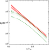 |
Fig. 1. Examples of 20 linear, as defined by l = 1 − D/L ≥ 0.9 (red solid lines), and 20 nonlinear, l < 0.9 (green dashed lines), Qρ(r) for ellipticals in model 7. L and D are defined in Eqs. (10) and (11), respectively. |
4. Results
4.1. Linearity of log Q versus log r
We first consider whether the Q(r) and Qr(r) profiles are linear in logarithmic space. Figure 2 shows the fraction fl of MCMC chain elements that have l ≥ 0.9 (see Sect. 3) with the fl values listed in Table 2. Independently of the chosen model and galaxy type, all profiles are linear for over 95% of the MCMC chains for Qρ and Qr, ρ. The fl values of the Qρ and Qr, ρ profiles are almost identical. There is no clear dependence of fl on either the ρ(r) or the β(r) model chosen. Recall that we did not consider the models of Paper II that lead to linear β − γ relations to avoid biasing the linearity of the PPSD, since the PPSD and β − γ relations may be physically related.
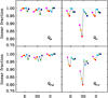 |
Fig. 2. Fraction of linear, l ≥ 0.9, relations deduced from the MCMC chain elements, for E, S0, and S tracers, in different models (color coded as in Table 1) for the sigv scaling, using total mass density profile (left) and tracer number density profiles (right), with total velocity dispersion (top) and radial velocity dispersion (bottom). Error bars are smaller than the symbol sizes. |
Q and Qr profiles: fl and slopes for the sigv scaling.
The Qν and Qr, ν profiles are also linear for over 90% of the MCMC chain elements, independently of the chosen model, but only when either ellipticals or spirals are considered. When considering S0, the fl values for the Qν and Qr, ν profiles can be as low as ≃0.80. Models with gNFW ρ(r) have lower values of fl when considering S0. The fl values of the Qν and Qr, ν profiles are very similar.
Combining all three morphological classes, the linear fractions for Qρ and Qr, ρ are maximal for model 15e (n = 6 Einasto with gOM anisotropy). Similarly, for Qν and Qr, ν, the linear fractions are maximal for model 12 (NFW with Tiret anisotropy).
4.2. Slopes
We then fit straight lines to log Q and log Qr vs. log(r/r−2), for the MCMC chain elements for which l ≥ 0.9 (nonlinear profiles are not considered as the straight line slope is not a useful statistic for them). We show the distributions of the best-fit logarithmic slopes of Q(r) in Fig. 3 (left panel: Qρ, right panel: Qν) and of Qr(r) in Fig. 4. The slope distributions do not differ in a significant way from one model to another and have similar unimodal shapes for all profiles.
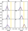 |
Fig. 3. Marginal distributions of the logarithmic slopes of the linear (l ≥ 0.9) Q profiles, for different morphological classes (E, S0, S in the top, middle, and bottom panel, respectively) using different models (color coded as in Table 1), for sigv scaling. Left panels: Qρ; right panels: Qν. Grey (respectively yellow) shadings indicate the simulation-based prediction for the slope of DM tracers (respectively subhalos), −1.84 ± 0.025 (respectively −1.29 ± 0.03). |
We compare our observational results with the predictions for DM particles from cosmological simulations, adopting the slope values that Dehnen & McLaughlin (2005) obtained from the DM-only cosmological simulations of Diemand et al. (2004a,b), −1.84 and −1.92 for Q(r) and Qr(r), respectively, with uncertainties of 0.025 and 0.05, respectively, to account for the scatter among the values found in different studies, that include both DM-only and hydrodynamical simulations (Taylor & Navarro 2001; Rasia et al. 2004; Dehnen & McLaughlin 2005; Knollmann et al. 2008). We also compare the observational results with the only available predictions for subhalos in cosmological hydrodynamical simulations, those of Marini et al. (2021), who found a Q(r) slope of −1.29 ± 0.03 (the authors did not study Qr(r)).
Figure 5 shows the biweight means and dispersions of the marginal distributions of the PPSD slopes (total and radial) shown in Figs. 3 and 4, compared with the simulation-based values. We also provide the average and dispersion of the logarithmic slopes of the linear Q, Qr profiles for all models and all galaxy types in Table 2. Our results do not depend in a significant way on the assumed model for ρ(r) and β(r). In fact, the average logarithmic slopes of the Q and Qr profiles for a given galaxy type are very similar across different models, and the dispersions of the average slope values of the seven models is much smaller than the dispersion in the values of the slopes obtained from the MCMC of any individual model (see rows labeled ‘mean’ in Table 2).
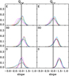 |
Fig. 4. Same as Fig. 3, but for Qr instead of Q. Gray shadings indicate the simulation-based prediction for the slope of DM tracers, −1.92 ± 0.05. |
Both for ellipticals and spirals, and also marginally for S0s, the logarithmic slopes of the linear Qρ and Qr, ρ profiles are consistent with the simulation-based prediction for DM tracers for all models (Fig. 5). The Qν and Qr, ν profile slopes for ellipticals are consistent with those of simulations based on DM tracers, while the corresponding slopes for spirals are not. The Qν slopes for S0s are also inconsistent with the simulation-based predictions based on DM tracers for all models, while the Qr, ν profile slopes for S0s are marginally consistent with the same simulation predictions (thanks to larger dispersions). Interestingly, the spiral Qν profile slopes are in agreement with the simulation-based prediction for subhalos, while the elliptical and S0 Qν profiles are not.
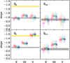 |
Fig. 5. Average and dispersion of the Q profile logarithmic slope and the simulation-based predictions for DM tracers (grey shading), −1.84 ± 0.025 for Q(r) and −1.92 ± 0.05 for Qr(r), and for subhalos (yellow shading), −1.29 ± 0.03, for different morphological classes (indicated on the x axis), in different models (color coded as in Fig. 2 and Table 1). Only linear (l ≥ 0.9) profiles are considered. |
5. Discussion
We discuss in turn our results on sigv stacks and on the other two stacks (num and tempX).
5.1. Discussion of results on sigv stacked clusters
Most Qρ and Qr, ρ profiles are very close to power-law relations: 96% of all models and galaxy types show PPSDs with linearity l > 0.9 (see Fig. 2, left panels, and Table 2). The large majority of MCMC chain elements predict power-law Qρ(r) and Qr, ρ(r) with average slopes in very good agreement and fully consistent with the simulation-based expectations using DM particles as tracers, but slightly flatter for S0s than for ellipticals and spirals (see Fig. 5, top-left panel). Our results support the findings of several studies based on both DM-only and hydrodynamical simulations (Taylor & Navarro 2001; Rasia et al. 2004; Dehnen & McLaughlin 2005; Ludlow et al. 2010; Navarro et al. 2010), and of previous observational studies (Biviano et al. 2013, 2016, 2021; Munari et al. 2014), and do not support claims against the power-law behavior of Q(r) (Nadler et al. 2017). Since our results are based on a stack cluster, we can neither confirm nor reject the numerical result of Schmidt et al. (2008) against the universality of Q(r) across different cosmological halos. However, for none of the three galaxy classes do the Qρ(r) slopes agree with those obtained for subhalos in numerical simulations (Marini et al. 2021).
If both Q(r) and Qr(r) are power laws, of respective slopes α and α + Δα, then their ratio ℛ = Qr/Q = (3 − 2 β)3/2 should also be a power law of slope Δα. For the Tiret and gOM anisotropy models (Eq. (8)), one then expects
where y = r/rβ. Equation (12) indicates that ℛ varies from one constant value, ℛ0 = 3 − 2 β0, at small radii, to another constant value, ℛ∞ = 3 − 2 β∞, at large radii. Therefore, Qr/Q cannot be a power law over the full range of radii (unless β∞ = β0).
If one restricts the analysis to a narrow range of radii around r = rβ, one expects a quasi-linear behavior obtained by a series expansion of ℛ(y) in Eq. (12):

The zeroth order term is positive since β < 1 by definition. The first order term is proportional to δ, and is negative for β∞ > β0 but positive otherwise. Hence, the transition of Qr/Q from ℛ0 at small radii to ℛ∞ at large radii is smoother for low δ anisotropy profiles. This is illustrated in Fig. 6, which shows that the gOM model (δ = 2) is less linear than the Tiret (δ = 1) model. In turn, this would indicate that the fraction of linear models should be higher with Tiret anisotropy than for similar mass models with gOM anisotropy. However, in practice, the necessary nonlinearity of Qr/Q is not a worry, because the nonlinearity range of Qr/Q is smaller than the nonlinearity range of either Q(r) or Qr(r), because the logarithmic slopes of Q(r) and Qr(r) are similar (Table 2). For example, if Q(r) were perfectly linear (l = 1), then Qr would have a linearity l = 0.997 and 0.992 for the Tiret and gOM anisotropy models, respectively, hence much greater than our threshold of 0.9 for linear models.
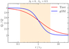 |
Fig. 6. Illustration of the nonlinearity of Qr/Q in Tiret and gOM anisotropy models (Eq. (12) with δ = 1 and 2, respectively). Our analysis was limited to the radii in the shaded region. |
It might at first appear surprising that Qρ and Qr, ρ should have similar slopes for the three morphological classes, given that the three classes have different line-of-sight velocity dispersion profiles (Paper I) and different β(r) (Paper II). The similarity of Qρ and Qr, ρ for the three classes then imply that they also have similar σ(r) and σr(r) and that the observed differences in their line-of-sight velocity dispersion profiles (Paper I) and β(r) (Paper II) is compensated by their different ν(r) (see Eqs. (2), (3), and Paper I).
One expects larger differences between the Qν(r) profiles of different morphological classes, because Qν is proportional to the number density of that class, and the number concentrations of the best-fit NFW models of each class differ significantly (Paper I). Indeed, the PPSDs of Qν and Qr, ν are increasingly shallower when moving from ellipticals to S0s to spirals (bottom panels of Fig. 5), even if these profiles are also quite close to power-law relations, with fl ≳ 0.8 for all models and all galaxy types (see Fig. 2, right panels, and Table 2). At variance with Qρ and Qr, ρ, only for ellipticals is there a good agreement between the observed Qν and Qr, ν slopes and the expected values from simulations using DM particles as tracers (bottom panels of Fig. 5). This is not surprising, given that ν(r)≈ρ(r) for ellipticals, but not for the other two types (Paper II).
Interestingly, the logarithmic slope of Qν(r) for spirals is very similar to the one found by Marini et al. (2021) for subhalos in cluster-size halos in cosmological hydrodynamical simulations (see bottom-left panel of Fig. 5). This similarity is probably related to the more extended radial distributions of spirals on one hand (Paper I) and of subhalos on the other (Marini et al. 2021). One should note that subhalos in dark matter only cosmological simulations of the same resolution show instead that the power-law dynamical entropy turns to flat inside half a virial radius.
The more extended subhalo number density profile, if not due to numerical effects (van den Bosch & Ogiya 2018), can be explained in several ways. Strong cluster tides at pericenter remove mass from infalling subhalos (Merritt 1983), as seen in simulations (e.g., Hayashi et al. 2003; Saro et al. 2006; Springel et al. 2008). Note again that the steeper dynamical entropy (hence steeper Qν) for the subhalos in hydrodynamical simulations relative to those in dark matter only ones suggests that the dissipative nature of gas leads to more concentrated subhalos that are more resilient to cluster tides. Such tides will remove mass from those subhalos that traverse the inner regions of clusters, causing (some of) the galaxies associated with them to fall below the data luminosity threshold. But tides affect all classes of galaxies, not just spirals. Alternatively, ram pressure stripping of the gas of spiral galaxies will strangle their subsequent star formation, leading to lower luminosities than gas-poor galaxies with the same orbits (Gunn & Gott 1972; Boselli et al. 2016). Another explanation may lie in temporal segregation instead of spatial segregation. If spiral galaxies are rapidly transformed into S0s and progressively into ellipticals (as argued, e.g., in Paper II), then S0s and ellipticals are the end products of galaxies that entered in the cluster earlier, most probably from lower apocenters. Thus the radial distribution of spirals is much more extended than S0s and ellipticals, leading to the shallower Qν slope of spirals. However, spirals are not expected to be the dominant morphological class in simulated cluster subhalos. Therefore, the good agreement between the Qν slopes of observed spirals and simulated subhalos remains an open question.
Our results for the Qν and Qr, ν profiles agree with those obtained from analysis of observations of Capasso et al. (2019), who determined Qν(r) for passive galaxies only, but not with Munari et al. (2015) and Aguerri et al. (2017), who found Qν(r) to be consistent with the simulation-based expectations by Dehnen & McLaughlin (2005), for all classes of galaxies in two nearby clusters. Perhaps, thanks to our large data set, we are able to detect significant differences that were not visible in individual cluster analyses because of limited statistics.
When comparing Qρ, Qr, ρ versus Qν, Qr, ν, we should take into account that we forced the NFW model for ν(r), but allowed three different models for ρ(r) (see Table 1). However, our results are very insensitive to the choice of the ρ(r) model, and models 12 and 15, that use NFW for ρ(r), behave very similarly to all the others. Our analysis then suggests that the ρ-based definition of Q and Qr is more fundamental than that based on ν, even if, observationally, Qρ and Qr, ρ are derived using inhomogeneous quantities, as ρ(r) refers to the distribution of total matter, dominated by DM, and σ, σr to the velocity dispersion of galaxies.
To interpret our results, we note that recent numerical simulations (Colombi 2021) show that the power-law Qρ and Qr, ρ profiles are established very early on for cluster DM, during the violent relaxation phase, possibly because of a tendency of the system toward a state of minimal entropy (He & Kang 2010). As galaxies enter the cluster gravitational potential well, their orbits and spatial distributions may evolve to reach the same state of dynamical entropy (∝Q−2.3), leading to the same Qρ and Qr, ρ as that of DM. Since the spatial distribution of ellipticals is similar to that of the total matter, we argue that the bulk motions of ellipticals experienced the same process of violent relaxation as the total matter, that is their progenitors (perhaps with different morphologies) were present at the time of cluster formation.
Violent relaxation at cluster formation cannot be the process shaping the PPSD profiles of S0s and spirals. Spirals have probably entered the cluster within the last ∼2 to 3 Gyr, after which they are morphologically transformed to S0s and/or ellipticals (e.g., Larson et al. 1980; Couch et al. 1998; see also Paper II), and quenched by the cluster environment (e.g., Poggianti et al. 2004; Haines et al. 2013), with indications that morphological transformation precedes star formation quenching (Sampaio et al. 2022). There is also observational evidence that S0s are not a pristine cluster population (Postman et al. 2005; Smith et al. 2005; Desai et al. 2007). The deviation of the S0s and spirals Qν and Qr, ν profiles from simulation-based expectations for DM particles is probably an indication that their PPSD is achieved in a different way from ellipticals. S0s are an intermediate population between that of ellipticals and spirals, in terms of their PPSD. If S0s originate from spirals through some environmental process, such a process could also be responsible for the gradual PPSD evolution from that of spirals to that of ellipticals (Paper I). However, no such evolution is seen for the subhalo PPSD in cluster-sized halos from cosmological simulation (I. Marini, private comm.).
While the Qν and Qr, ν profiles of S0s and spirals differ from the simulation-based expectations for DM particles, it is surprising that their Qρ and Qr, ρ do not. Then, violent relaxation cannot be the only process conducive to the observed Qρ and Qr, ρ power-law slopes. According to Dehnen & McLaughlin (2005) the dynamical process that leads to the Qr power-law behavior can be understood in terms of the Jeans equation of dynamical equilibrium by assuming that β is linearly related to γ. In their model, the logarithmic slope αr of Qr, must be related to the central orbital anisotropy β0 by
In Fig. 7, we show the distributions of the MCMC chain elements in the αr − β0 plane, separately for the three morphological classes. Ellipticals follow quite closely Dehnen & McLaughlin (2005)’s relation (Eq. (14), above), and so do spirals for most – but not all – models, while S0s do not. So the dynamical process that leads to the observed Qρ and Qr, ρ power-law slopes, might indeed be the one suggested by Dehnen & McLaughlin (2005) for spirals. Even if spirals are only recently accreted to the cluster, and cannot be considered fully dynamically relaxed in the cluster potential, the analysis of semi-analytical simulations indicate that they obey the Jeans equation of dynamical equilibrium (Aguirre Tagliaferro et al. 2021), so the above interpretation of Dehnen & McLaughlin (2005) can apply to them.
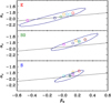 |
Fig. 7. Distributions of Qr, ρ logarithmic slopes vs. central velocity anisotropy, β0 for the E (top panel), S0 (middle panel), and S (bottom panel) classes. Dots indicate the peaks of the density distribution of the MCMC chain elements in this diagram, for the different models (color coded as in Table 1). The contour contains 68% of the MCMC chain elements for model 15e (navy blue). We omit the contours of the other models for the sake of clarity. The solid line is the relation αr = − 35/18 + 2/9 β0 from Dehnen & McLaughlin (2005). |
On the other hand, the process described by Dehnen & McLaughlin (2005) does not seem to be a viable explanation for the consistency of the Qρ(r) and Qr, ρ(r) of S0s with simulation-based expectations for DM particles, as they appear to depart from the relation between PPSD slope and inner velocity anisotropy of Eq. (14). However, among the three morphological classes considered here, S0s show the strongest, albeit not very significant, deviation of the Qρ and Qr, ρ profile slopes from the simulation-based expectations (see Fig. 5). In Paper I we argued that S0s are a transition class between the spiral and elliptical classes, as far as their dynamics within the cluster is concerned. Their velocity dispersion profile appears to be close to that of spirals near the center and to that of ellipticals in the outer regions. This is true not only for the line-of-sight velocity dispersion profile, as we noted in Paper I already, but also when considering the total, σ(r), and radial, σr(r), profiles, as shown in Fig. 8. On the other hand, the ellipticals and spirals have very similar σ(r) and σr(r), except for different normalizations, as expected from the similarity of the logarithmic slopes of their Qρ and Qr, ρ profiles.
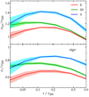 |
Fig. 8. Velocity dispersion profiles: total (top panel) and radial component (bottom panel) for the ellipticals (solid red line and pink shading), S0s (dash-dotted green line and light green shading), and spirals (dashed blue line and cyan shading). The curves are the biweight averages over all seven models and the shadings are the dispersions among the seven models. |
It is possible that S0s are not a homogeneous class, but a mixed bag of galaxies that formed in different ways at different epochs of the cluster evolution, namely by ram pressure stripping of disks (Gunn & Gott 1972) and by merger growth of bulges (van den Bergh 1990). The two formation channels of S0s is suggested by studies of their internal structure, gas content, and kinematics (Coccato et al. 2020; Deeley et al. 2020, 2021), with disk stripping dominating in clusters and bulge growth in isolated galaxies (Deeley et al. 2020). So maybe the Qρ and Qr, ρ profiles of S0s agree with simulation-based expectations (albeit less well than those of ellipticals and spirals) because some S0s followed the dynamical history of ellipticals and some that of spirals.
We are thus led to suggest the following conclusion. Both Qν(r) and Qr, ν(r) keep memory of the accretion time of the cluster population, while Qρ(r) and Qr, ρ(r) are related to the dynamical equilibrium of the population within the cluster potential, that is not necessarily achieved via violent relaxation only.
5.2. Discussion of results on num and tempX stacked clusters
We now turn to the results of our analysis using the other two stacking methods (to determine the virial radii): num (richness) and tempX (X-ray temperature). The tables and figures are displayed in Appendix A.
Figures A.1 and A.2 show the linear fractions, fl, of Q and Qr profiles from the MCMC chain elements for the num and tempX scalings, respectively. One sees fl values as low or even a bit lower than 40%, depending on the model and the galaxy type, considerably lower than the > 95% obtained for the sigv scaling. This indicates that the ensemble cluster built using the sigv scaling has a (projected) phase-space distribution that is more similar to that of simulated halos, than the ensemble clusters built using the other two scalings. Another remarkable difference of the num and tempX scalings is that fl for Qr profiles is on average lowest for ellipticals among the three morphological classes, while it is lowest for S0s when considering the sigv scaling.
The marginal distributions of the best-fit logarithmic slopes of Q(r) and Qr(r) (considering only linear profiles) are displayed in Figs. A.3 and A.4 for the num scaling, respectively, (left panel: Qρ, right panel: Qν) and in Figs. A.5 and A.6 for the tempX scaling. For the num scaling, we show in Figs. A.7 the averages and dispersions of the Q(r) and Qr(r) logarithmic slopes obtained on the MCMC chain elements (considering only linear profiles). Figure A.8 shows the corresponding quantities for the tempX scaling. We also provide the average and dispersion of the logarithmic slopes of the Q and Qr profiles for all MCMC chain elements with linear PPSDs, for all models and all galaxy types in Tables A.1 and A.2 for the num and tempX scaling, respectively.
The results for the slopes of Qρ(r) and Qr, ρ(r) obtained using the num and tempX scalings are generally within one standard deviation of the results obtained using the sigv scaling. This is illustrated in Fig. 9, where we show the differences Δ between both the num- and the tempX-scaling slopes and the sigv-scaling slope, considering only linear profiles among all MCMC chains. The differences are shown in units of the quadratically combined dispersions of the slopes, σslopes. These differences are not statistically significant. The most significant differences come from the Qr(r) slopes of ellipticals and spirals, which are almost identical to that of S0s, and they are all somewhat flatter than the expected relations from numerical simulations (see the top-right panels of Figs. A.7 and A.8). Moreover, the Q(r) slopes of S0s are intermediate between those of ellipticals and spirals, unlike what was found with the sigv scaling.
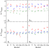 |
Fig. 9. Difference Δ between the logarithmic slopes obtained for the num (circles) and tempX (crosses) scalings and the slopes obtained for the sigv scaling, for the three morphological classes, ellipticals (red), S0s (green), spirals (blue), for the different models (x axis). The Δ differences are given in units of the quadratically combined dispersions of the slopes. |
S0s also appear to be an intermediate class between ellipticals and spirals in the β0 − αr diagram. As seen in Figs. A.9 and A.10, it is not the S0s but the spirals that are the most distant from the expected relation, contrary to what was found using the sigv scaling. Moreover, the velocity dispersion profiles of S0s show less of a transition from those of spirals at small radii to those of ellipticals near the virial radius (Figs. A.11 and A.12) than is the case for the sigv stack (Fig. 8). The results for the num and tempX scalings therefore suggest that S0s are an intermediate class between ellipticals and spirals, rather than a mixed class. Another remarkable difference with respect to the sigv scaling, is that the β0 − αr relation of Eq. (14) is not obeyed by any of the three morphological classes. This means we cannot rely on Dehnen & McLaughlin (2005)’s explanation for why later accreted galaxy populations such as the spirals, and to a lesser extent, S0s, have Q(r) profiles consistent with those of DM particles.
Not only are the Qr, ρ profiles obtained using the num and tempX scalings flatter than simulations predict for DM particles, they are in some cases even flatter than the Qρ profiles. This can happen if the velocity anisotropy profiles are more radial near the center than at the cluster virial radius, as illustrated in Fig. 10. Anisotropy profiles of this kind are not typical of either simulated cluster-size halos (e.g., Ascasibar & Gottlöber 2008; Mamon et al. 2010; Lemze et al. 2012; Munari et al. 2013; Lotz et al. 2019) or real clusters (e.g., Natarajan & Kneib 1996; Biviano & Katgert 2003; Lemze et al. 2009; Wojtak & Łokas 2010; Biviano et al. 2013; Annunziatella et al. 2016; Aguerri et al. 2017; Capasso et al. 2019). This suggests that one should take the results obtained using the num and tempX scalings with some caution.
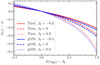 |
Fig. 10. Difference of mean logarithmic slope of Qr, ρ with logarithmic slope of Qρ (here α = −1.8) as a function of difference in velocity anisotropies between virial radius and 0, using Eqs. (8) and (12) for c = r200/rβ = 4. Changing c and α has negligible effect on the curves. This indicates that Qr, ρ is steeper than Qρ unless β(r200) < β0. |
In conclusion, while the results we obtain for the num and tempX scalings are not significantly different from those obtained for the sigv scaling, they are more distant from the predictions from numerical simulations for what concerns the linearity of the profiles and the slope of Qr, ρ(r). If the power-law behavior of Q(r) and Qr(r) could be theoretically motivated, the better adherence of the sigv-based profiles to the power-law behavior would suggest that the velocity dispersion is a better r200 estimator than either the cluster richness or its X-ray temperature, at least for the WINGS cluster data set.
6. Summary and conclusions
We determined the average Q and Qr profiles of nearby galaxy clusters, using either total mass density ρ(r) or tracer number density ν(r), as well as the velocity dispersion profiles of three galaxy classes, ellipticals, S0s, and spirals. For this, we have used the results of the MCMC analysis of the kinematics of a velocity-dispersion-based (sigv) stack of 54 regular clusters (Paper I) from the WINGS data set (Fasano et al. 2006; Cava et al. 2009; Moretti et al. 2014) performed with the MAMPOSSt code in Paper II.
We find that Qρ(r) and Qr, ρ(r) are very close to the power-law relations predicted by numerical simulations for DM particles (Taylor & Navarro 2001; Rasia et al. 2004; Dehnen & McLaughlin 2005), at least in a range from a few percent to one virial radius. On the other hand, Qν(r) and Qr, ν(r) only agree with the simulation-based predictions for DM particles for the ellipticals, and they deviate from the simulation-based predictions for the S0s and spirals marginally and significantly, respectively. Only the spiral Qν(r) is similar to that of subhalos in halos from cosmological hydrodynamical simulations.
We checked our results on two different stacks of the same data set, based on richness (num) and gas temperature (tempX) scalings. While we find a lower fraction of power-law Q and Qr profiles, the average slopes of these profiles are not significantly different from those obtained for the sigv scaling.
We argue that our results based on the sigv scaling support a scenario in which Qρ(r) and Qr, ρ(r) are either established early on, during the cluster violent relaxation phase, for the DM and ellipticals, or established subsequently, for spirals by adapting their orbital and spatial distribution as they move toward dynamical equilibrium in the cluster potential. S0s might be a mixed class, with part of them following the dynamical history of ellipticals and the other part following that of spirals, as suggested by our analysis of the sigv stack, or an intermediate class between spirals and ellipticals as is consistent with our analysis of the num and tempX stacks. On the other hand, Qν(r) and Qr, ν(r) are not universal, and they depend on the time of accretion of the tracer population in the cluster. In conclusion, our results give strong observational support to the simulation-based power-law Q and Qr profiles when they are defined using total mass density ρ(r), rather than the tracer number density ν(r).
The Einasto model was first proposed by Einasto (1965) in a completely different context.
Acknowledgments
We thank the referee for her or his constructive and pertinent comments. We also acknowledge the WINGS team for their active and precious collaboration. We thank Ilaria Marini for useful discussions. G.A.M. and A.B. are grateful to the IFPU and IAP, respectively for their hospitality during part of this collaboration.
References
- Aguerri, J. A. L., Agulli, I., Diaferio, A., & Dalla Vecchia, C. 2017, MNRAS, 468, 364 [NASA ADS] [CrossRef] [Google Scholar]
- Aguirre Tagliaferro, T., Biviano, A., De Lucia, G., Munari, E., & Garcia Lambas, D. 2021, A&A, 652, A90 [NASA ADS] [CrossRef] [EDP Sciences] [Google Scholar]
- Annunziatella, M., Mercurio, A., Biviano, A., et al. 2016, A&A, 585, A160 [NASA ADS] [CrossRef] [EDP Sciences] [Google Scholar]
- Arora, A., & Williams, L. L. R. 2020, ApJ, 893, 53 [NASA ADS] [CrossRef] [Google Scholar]
- Ascasibar, Y., & Gottlöber, S. 2008, MNRAS, 386, 2022 [CrossRef] [Google Scholar]
- Ascasibar, Y., Yepes, G., Gottlöber, S., & Müller, V. 2004, MNRAS, 352, 1109 [NASA ADS] [CrossRef] [Google Scholar]
- Austin, C. G., Williams, L. L. R., Barnes, E. I., Babul, A., & Dalcanton, J. J. 2005, ApJ, 634, 756 [NASA ADS] [CrossRef] [Google Scholar]
- Barnes, E. I., Williams, L. L. R., Babul, A., & Dalcanton, J. J. 2007, ApJ, 654, 814 [NASA ADS] [CrossRef] [Google Scholar]
- Bertschinger, E. 1985, ApJS, 58, 39 [Google Scholar]
- Binney, J. 1980, MNRAS, 190, 873 [NASA ADS] [CrossRef] [Google Scholar]
- Biviano, A., & Katgert, P. 2003, Ap&SS, 285, 25 [NASA ADS] [CrossRef] [Google Scholar]
- Biviano, A., Rosati, P., Balestra, I., et al. 2013, A&A, 558, A1 [Google Scholar]
- Biviano, A., van der Burg, R. F. J., Muzzin, A., et al. 2016, A&A, 594, A51 [NASA ADS] [CrossRef] [EDP Sciences] [Google Scholar]
- Biviano, A., van der Burg, R. F. J., Balogh, M. L., et al. 2021, A&A, 650, A105 [NASA ADS] [CrossRef] [EDP Sciences] [Google Scholar]
- Boselli, A., Roehlly, Y., Fossati, M., et al. 2016, A&A, 596, A11 [NASA ADS] [CrossRef] [EDP Sciences] [Google Scholar]
- Brown, S. T., McCarthy, I. G., Diemer, B., et al. 2020, MNRAS, 495, 4994 [NASA ADS] [CrossRef] [Google Scholar]
- Butsky, I., Macciò, A. V., Dutton, A. A., et al. 2016, MNRAS, 462, 663 [NASA ADS] [CrossRef] [Google Scholar]
- Capasso, R., Saro, A., Mohr, J. J., et al. 2019, MNRAS, 482, 1043 [NASA ADS] [CrossRef] [Google Scholar]
- Cava, A., Bettoni, D., Poggianti, B. M., et al. 2009, A&A, 495, 707 [NASA ADS] [CrossRef] [EDP Sciences] [Google Scholar]
- Cava, A., Biviano, A., Mamon, G. A., et al. 2017, A&A, 606, A108 [NASA ADS] [CrossRef] [EDP Sciences] [Google Scholar]
- Chae, K.-H. 2014, ApJ, 788, L15 [NASA ADS] [CrossRef] [Google Scholar]
- Coccato, L., Jaffé, Y. L., Cortesi, A., et al. 2020, MNRAS, 492, 2955 [Google Scholar]
- Colombi, S. 2021, A&A, 647, A66 [NASA ADS] [CrossRef] [EDP Sciences] [Google Scholar]
- Couch, W. J., Barger, A. J., Smail, I., Ellis, R. S., & Sharples, R. M. 1998, ApJ, 497, 188 [NASA ADS] [CrossRef] [Google Scholar]
- Deeley, S., Drinkwater, M. J., Sweet, S. M., et al. 2020, MNRAS, 498, 2372 [Google Scholar]
- Deeley, S., Drinkwater, M. J., Sweet, S. M., et al. 2021, MNRAS, 508, 895 [NASA ADS] [CrossRef] [Google Scholar]
- Dehnen, W., & McLaughlin, D. E. 2005, MNRAS, 363, 1057 [Google Scholar]
- Desai, V., Dalcanton, J. J., Aragón-Salamanca, A., et al. 2007, ApJ, 660, 1151 [NASA ADS] [CrossRef] [Google Scholar]
- Diemand, J., Moore, B., & Stadel, J. 2004a, MNRAS, 352, 535 [NASA ADS] [CrossRef] [Google Scholar]
- Diemand, J., Moore, B., & Stadel, J. 2004b, MNRAS, 353, 624 [NASA ADS] [CrossRef] [Google Scholar]
- Dressler, A., & Shectman, S. A. 1988, AJ, 95, 985 [Google Scholar]
- Dutton, A. A., & Macciò, A. V. 2014, MNRAS, 441, 3359 [Google Scholar]
- Einasto, J. 1965, Trudy Astrofizicheskogo Instituta Alma-Ata, 5, 87 [NASA ADS] [Google Scholar]
- Faltenbacher, A., Hoffman, Y., Gottlöber, S., & Yepes, G. 2007, MNRAS, 376, 1327 [NASA ADS] [CrossRef] [Google Scholar]
- Fasano, G., Marmo, C., Varela, J., et al. 2006, A&A, 445, 805 [NASA ADS] [CrossRef] [EDP Sciences] [Google Scholar]
- Gelman, A., & Rubin, D. B. 1992, Stat. Sci., 7, 457 [Google Scholar]
- Gott, J. R. 1975, ApJ, 201, 296 [Google Scholar]
- Gunn, J. E. 1977, ApJ, 218, 592 [NASA ADS] [CrossRef] [Google Scholar]
- Gunn, J. E., & Gott, J. R. 1972, ApJ, 176, 1 [NASA ADS] [CrossRef] [Google Scholar]
- Haines, C. P., Pereira, M. J., Smith, G. P., et al. 2013, ApJ, 775, 126 [NASA ADS] [CrossRef] [Google Scholar]
- Hansen, S. H., & Moore, B. 2006, New Astron., 11, 333 [NASA ADS] [CrossRef] [Google Scholar]
- Hansen, S. H., & Stadel, J. 2006, J. Cosmol. Astropart. Phys., 05, 014 [NASA ADS] [Google Scholar]
- Hayashi, E., Navarro, J. F., Taylor, J. E., Stadel, J., & Quinn, T. 2003, ApJ, 584, 541 [Google Scholar]
- He, P., & Kang, D.-B. 2010, MNRAS, 406, 2678 [NASA ADS] [CrossRef] [Google Scholar]
- Henriksen, R. N. 2006, MNRAS, 366, 697 [NASA ADS] [CrossRef] [Google Scholar]
- Hoffman, Y., Romano-Díaz, E., Shlosman, I., & Heller, C. 2007, ApJ, 671, 1108 [NASA ADS] [CrossRef] [Google Scholar]
- Knollmann, S. R., Knebe, A., & Hoffman, Y. 2008, MNRAS, 391, 559 [NASA ADS] [CrossRef] [Google Scholar]
- Lapi, A., & Cavaliere, A. 2009, ApJ, 692, 174 [NASA ADS] [CrossRef] [Google Scholar]
- Lapi, A., & Cavaliere, A. 2011, ApJ, 743, 127 [Google Scholar]
- Larson, R. B., Tinsley, B. M., & Caldwell, C. N. 1980, ApJ, 237, 692 [Google Scholar]
- Lemze, D., Broadhurst, T., Rephaeli, Y., Barkana, R., & Umetsu, K. 2009, ApJ, 701, 1336 [NASA ADS] [CrossRef] [Google Scholar]
- Lemze, D., Wagner, R., Rephaeli, Y., et al. 2012, ApJ, 752, 141 [NASA ADS] [CrossRef] [Google Scholar]
- Lewis, I., Balogh, M., De Propris, R., et al. 2002, MNRAS, 334, 673 [NASA ADS] [CrossRef] [Google Scholar]
- Lotz, M., Remus, R.-S., Dolag, K., Biviano, A., & Burkert, A. 2019, MNRAS, 488, 5370 [NASA ADS] [CrossRef] [Google Scholar]
- Ludlow, A. D., Navarro, J. F., Springel, V., et al. 2010, MNRAS, 406, 137 [NASA ADS] [CrossRef] [Google Scholar]
- Lynden-Bell, D. 1967, MNRAS, 136, 101 [Google Scholar]
- Ma, D., & He, P. 2009, Int. J. Mod. Phys. D, 18, 477 [NASA ADS] [CrossRef] [Google Scholar]
- MacMillan, J. D., Widrow, L. M., & Henriksen, R. N. 2006, ApJ, 653, 43 [Google Scholar]
- Mamon, G. A., & Łokas, E. L. 2005, MNRAS, 363, 705 [Google Scholar]
- Mamon, G. A., Biviano, A., & Murante, G. 2010, A&A, 520, A30 [NASA ADS] [CrossRef] [EDP Sciences] [Google Scholar]
- Mamon, G. A., Biviano, A., & Boué, G. 2013, MNRAS, 429, 3079 [Google Scholar]
- Mamon, G. A., Cava, A., Biviano, A., et al. 2019, A&A, 631, A131 [NASA ADS] [CrossRef] [EDP Sciences] [Google Scholar]
- Manrique, A., Raig, A., Salvador-Solé, E., Sanchis, T., & Solanes, J. M. 2003, ApJ, 593, 26 [NASA ADS] [CrossRef] [Google Scholar]
- Marini, I., Saro, A., Borgani, S., et al. 2021, MNRAS, 500, 3462 [Google Scholar]
- Merritt, D. 1983, ApJ, 264, 24 [NASA ADS] [CrossRef] [Google Scholar]
- Merritt, D. 1985, MNRAS, 214, 25P [NASA ADS] [CrossRef] [Google Scholar]
- Moretti, A., Poggianti, B. M., Fasano, G., et al. 2014, A&A, 564, A138 [NASA ADS] [CrossRef] [EDP Sciences] [Google Scholar]
- Munari, E., Biviano, A., Borgani, S., Murante, G., & Fabjan, D. 2013, MNRAS, 430, 2638 [Google Scholar]
- Munari, E., Biviano, A., & Mamon, G. A. 2014, A&A, 566, A68 [NASA ADS] [CrossRef] [EDP Sciences] [Google Scholar]
- Munari, E., Biviano, A., & Mamon, G. A. 2015, A&A, 574, C1 [NASA ADS] [CrossRef] [EDP Sciences] [Google Scholar]
- Nadler, E. O., Oh, S. P., & Ji, S. 2017, MNRAS, 470, 500 [NASA ADS] [CrossRef] [Google Scholar]
- Natarajan, P., & Kneib, J.-P. 1996, MNRAS, 283, 1031 [NASA ADS] [CrossRef] [Google Scholar]
- Navarro, J. F., Frenk, C. S., & White, S. D. M. 1996, ApJ, 462, 563 [Google Scholar]
- Navarro, J. F., Ludlow, A., Springel, V., et al. 2010, MNRAS, 402, 21 [Google Scholar]
- Navarro, J. F., Hayashi, E., Power, C., et al. 2004, MNRAS, 349, 1039 [Google Scholar]
- Old, L., Skibba, R. A., Pearce, F. R., et al. 2014, MNRAS, 441, 1513 [Google Scholar]
- Osipkov, L. P. 1979, Sov. Astron. Lett., 5, 42 [NASA ADS] [Google Scholar]
- Poggianti, B. M., Bridges, T. J., Komiyama, Y., et al. 2004, ApJ, 601, 197 [NASA ADS] [CrossRef] [Google Scholar]
- Postman, M., Franx, M., Cross, N. J. G., et al. 2005, ApJ, 623, 721 [Google Scholar]
- Pratt, G. W., Arnaud, M., Biviano, A., et al. 2019, Space Sci. Rev., 215, 25 [Google Scholar]
- Rasia, E., Tormen, G., & Moscardini, L. 2004, MNRAS, 351, 237 [NASA ADS] [CrossRef] [Google Scholar]
- Read, J. I., Mamon, G. A., Vasiliev, E., et al. 2021, MNRAS, 501, 978 [Google Scholar]
- Sampaio, V. M., de Carvalho, R. R., Ferreras, I., Aragón-Salamanca, A., & Parker, L. C. 2022, MNRAS, 509, 567 [Google Scholar]
- Saro, A., Borgani, S., Tornatore, L., et al. 2006, MNRAS, 373, 397 [NASA ADS] [CrossRef] [Google Scholar]
- Schmidt, K. B., Hansen, S. H., & Macciò, A. V. 2008, ApJ, 689, L33 [NASA ADS] [CrossRef] [Google Scholar]
- Smith, G. P., Treu, T., Ellis, R. S., Moran, S. M., & Dressler, A. 2005, ApJ, 620, 78 [NASA ADS] [CrossRef] [Google Scholar]
- Springel, V., Wang, J., Vogelsberger, M., et al. 2008, MNRAS, 391, 1685 [Google Scholar]
- Taylor, J. E., & Navarro, J. F. 2001, ApJ, 563, 483 [Google Scholar]
- Tiret, O., Combes, F., Angus, G. W., Famaey, B., & Zhao, H. S. 2007, A&A, 476, L1 [NASA ADS] [CrossRef] [EDP Sciences] [Google Scholar]
- van den Bergh, S. 1990, ApJ, 348, 57 [NASA ADS] [CrossRef] [Google Scholar]
- van den Bosch, F. C., & Ogiya, G. 2018, MNRAS, 475, 4066 [NASA ADS] [CrossRef] [Google Scholar]
- van der Marel, R. P. 1994, MNRAS, 270, 271 [NASA ADS] [CrossRef] [Google Scholar]
- Vass, I. M., Valluri, M., Kravtsov, A. V., & Kazantzidis, S. 2009, MNRAS, 395, 1225 [CrossRef] [Google Scholar]
- Wojtak, R., & Łokas, E. L. 2010, MNRAS, 408, 2442 [NASA ADS] [CrossRef] [Google Scholar]
- Zait, A., Hoffman, Y., & Shlosman, I. 2008, ApJ, 682, 835 [NASA ADS] [CrossRef] [Google Scholar]
- Zhao, H. 1996, MNRAS, 278, 488 [Google Scholar]
Appendix A: Results for the num and tempX scalings
In the main text of this paper, we provided the results for the velocity dispersion-based sigv scaling used to stack the clusters. Here we provide the results for the richness-based, num, and X-ray temperature-based, tempX scalings.
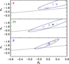 |
Fig. A.10. Same as Fig. 7, but for the tempX scaling. |
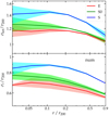 |
Fig. A.11. Same as Fig. 8, but for the num scaling. |
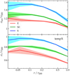 |
Fig. A.12. Same as Fig. 8, but for the tempX scaling. |
Q and Qr profiles: fl and slopes for the num scaling
Q and Qr profiles: fl and slopes for the tempX scaling
All Tables
All Figures
|
Fig. 1. Examples of 20 linear, as defined by l = 1 − D/L ≥ 0.9 (red solid lines), and 20 nonlinear, l < 0.9 (green dashed lines), Qρ(r) for ellipticals in model 7. L and D are defined in Eqs. (10) and (11), respectively. |
| In the text | |
|
Fig. 2. Fraction of linear, l ≥ 0.9, relations deduced from the MCMC chain elements, for E, S0, and S tracers, in different models (color coded as in Table 1) for the sigv scaling, using total mass density profile (left) and tracer number density profiles (right), with total velocity dispersion (top) and radial velocity dispersion (bottom). Error bars are smaller than the symbol sizes. |
| In the text | |
|
Fig. 3. Marginal distributions of the logarithmic slopes of the linear (l ≥ 0.9) Q profiles, for different morphological classes (E, S0, S in the top, middle, and bottom panel, respectively) using different models (color coded as in Table 1), for sigv scaling. Left panels: Qρ; right panels: Qν. Grey (respectively yellow) shadings indicate the simulation-based prediction for the slope of DM tracers (respectively subhalos), −1.84 ± 0.025 (respectively −1.29 ± 0.03). |
| In the text | |
|
Fig. 4. Same as Fig. 3, but for Qr instead of Q. Gray shadings indicate the simulation-based prediction for the slope of DM tracers, −1.92 ± 0.05. |
| In the text | |
|
Fig. 5. Average and dispersion of the Q profile logarithmic slope and the simulation-based predictions for DM tracers (grey shading), −1.84 ± 0.025 for Q(r) and −1.92 ± 0.05 for Qr(r), and for subhalos (yellow shading), −1.29 ± 0.03, for different morphological classes (indicated on the x axis), in different models (color coded as in Fig. 2 and Table 1). Only linear (l ≥ 0.9) profiles are considered. |
| In the text | |
|
Fig. 6. Illustration of the nonlinearity of Qr/Q in Tiret and gOM anisotropy models (Eq. (12) with δ = 1 and 2, respectively). Our analysis was limited to the radii in the shaded region. |
| In the text | |
|
Fig. 7. Distributions of Qr, ρ logarithmic slopes vs. central velocity anisotropy, β0 for the E (top panel), S0 (middle panel), and S (bottom panel) classes. Dots indicate the peaks of the density distribution of the MCMC chain elements in this diagram, for the different models (color coded as in Table 1). The contour contains 68% of the MCMC chain elements for model 15e (navy blue). We omit the contours of the other models for the sake of clarity. The solid line is the relation αr = − 35/18 + 2/9 β0 from Dehnen & McLaughlin (2005). |
| In the text | |
|
Fig. 8. Velocity dispersion profiles: total (top panel) and radial component (bottom panel) for the ellipticals (solid red line and pink shading), S0s (dash-dotted green line and light green shading), and spirals (dashed blue line and cyan shading). The curves are the biweight averages over all seven models and the shadings are the dispersions among the seven models. |
| In the text | |
|
Fig. 9. Difference Δ between the logarithmic slopes obtained for the num (circles) and tempX (crosses) scalings and the slopes obtained for the sigv scaling, for the three morphological classes, ellipticals (red), S0s (green), spirals (blue), for the different models (x axis). The Δ differences are given in units of the quadratically combined dispersions of the slopes. |
| In the text | |
|
Fig. 10. Difference of mean logarithmic slope of Qr, ρ with logarithmic slope of Qρ (here α = −1.8) as a function of difference in velocity anisotropies between virial radius and 0, using Eqs. (8) and (12) for c = r200/rβ = 4. Changing c and α has negligible effect on the curves. This indicates that Qr, ρ is steeper than Qρ unless β(r200) < β0. |
| In the text | |
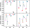 |
Fig. A.1. Same as Fig. 2, but for the num scaling. |
| In the text | |
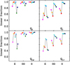 |
Fig. A.2. Same as Fig. 2, but for the tempX scaling. |
| In the text | |
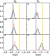 |
Fig. A.3. Same as Fig. 3, but for the num scaling. |
| In the text | |
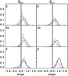 |
Fig. A.4. Same as Fig. 4, but for the num scaling. |
| In the text | |
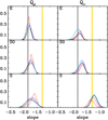 |
Fig. A.5. Same as Fig. 3 but for the tempX scaling. |
| In the text | |
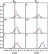 |
Fig. A.6. Same as Fig. 4, but for the tempX scaling. |
| In the text | |
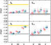 |
Fig. A.7. Same as Fig. 5, but for the num scaling. |
| In the text | |
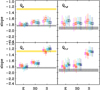 |
Fig. A.8. Same as Fig. 5, but for the tempX scaling. |
| In the text | |
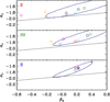 |
Fig. A.9. Same as Fig. 7, but for the num scaling. |
| In the text | |
|
Fig. A.10. Same as Fig. 7, but for the tempX scaling. |
| In the text | |
|
Fig. A.11. Same as Fig. 8, but for the num scaling. |
| In the text | |
|
Fig. A.12. Same as Fig. 8, but for the tempX scaling. |
| In the text | |
Current usage metrics show cumulative count of Article Views (full-text article views including HTML views, PDF and ePub downloads, according to the available data) and Abstracts Views on Vision4Press platform.
Data correspond to usage on the plateform after 2015. The current usage metrics is available 48-96 hours after online publication and is updated daily on week days.
Initial download of the metrics may take a while.