© ESO, 2011

1. Introduction

Subdwarf B (sdB) stars populate the blue extension of the horizontal branch (EHB) in a Hertzsprung-Russell diagram (Heber 1986). Their high temperatures (T_eff > 20   000   K) and high gravities (5 < log g < 6) correspond to an evolutionary state in between the red giant and white dwarf phases, although the detailed history is not well understood yet. An anomalously high mass loss rate at some point is needed to explain the hot subdwarf’s thin H-envelope, which prevents them from ascending the asymptotic giant branch (Dorman et al. 1993; D’Cruz et al. 1996). Mass transfer through binary interaction has been invoked as an explanation, because it is observationally supported by the high binary fraction of these objects in the field. The predominantly single sdBs that populate the EHB in globular clusters (Moni Bidin et al. 2011) can be explained by white dwarf mergers (Han et al. 2008).

Some sdB stars exhibit stellar oscillations. Indeed, long- (~1 h) and short-period (~10 min) pulsating sdBs can be distinguished (Kilkenny et al. 1997; Green et al. 2003), with a few hybrid objects showing both period regimes (Schuh et al. 2006; Oreiro et al. 2005; Lutz et al. 2009; Baran et al. 2011). Long-period oscillations are explained in terms of gravity modes (Fontaine et al. 2003), while short-period variations are attributed to pressure modes (Charpinet et al. 1997). Asteroseismic techniques can thus be applied to sdBs to retrieve information on their internal structure and rotation, and will eventually help to constrain their evolutionary formation channels (Hu et al. 2008).

Balloon 090100001 (Bal09 hereafter) is a hybrid sdB pulsator, with a rich frequency spectrum both at low and high frequencies. It also is the brightest sdB pulsator and has one of the highest amplitudes of oscillation, which makes Bal09 a very interesting object. Since the discovery of its pulsating nature (Oreiro et al. 2004), a multi-site photometric campaign was organized to unravel the complex frequency structure of the target during the 2005 summer (Baran et al. 2009), while a low-resolution time-resolved spectroscopy (Telting & Østensen 2006) and a high-resolution spectroscopy dataset enabled a mode identification (Telting et al. 2008; Baran et al. 2008). Mode identification was also attempted through multicolour photometry (Charpinet et al. 2008), while van Grootel et al. (2008) provide a seismic solution for Bal09.

An interesting feature concerning Bal09’s amplitude spectrum is that a triplet-like structure is resolved close to the dominant, single mode. Moreover, five components are also identified  ~25 μHz apart from the triplet. From these modes a frequency splitting of  ~1.5   μHz is derived. Assuming a canonical total mass M = 0.5M_⊙ and using the spectroscopic log g = 5.39 value, a rotational velocity between 1.5–2 km s^-1 (Telting et al. 2008) is obtained, in agreement with the typical low surface-rotation speed of single sdBs  (Geier et al. 2010).

Bal09 has been photometrically monitored after the main multi-site campaign in 2005 but no result has been published yet (Baran, private communication). A comparison of the 2004 and 2005 seasons allowed the detection of changes in the amplitudes of many modes. Amplitude variations are not uncommon among pulsating sdBs, as is discussed in Kilkenny (2010). On the other hand, small changes in the frequency splitting are found from one campaign to the other as well. Although close to the frequency resolution, the triplet components have moved in the right direction as if the rotation were varying. The quintuplet also varies in the same way, even though not all five components were resolved in 2004. Because it is unusual for a star to change its rotation on such a short time scale, a physical explanation for this phenomenon is yet to be found.

The aim of this work is to examine one possible mechanism that could explain the changes in the frequency splitting. We analyse here the possibility of angular momentum interchange between stellar rotation and internal waves. This scenario requires the existence of internal gravity waves with a dissipation mechanism or any other non-conservative process that eventually could lead to amplitude variations. This is the case in Bal09, where we can estimate the g-mode energies from the observations and hence quantify the angular momentum transport by waves.

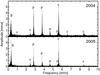Fig. 1 Comparison of the amplitude spectrum of Bal09 in 2004 and 2005 after removing the three highest peaks. Figure from Baran et al. (2009). P, g, and c stand for p-modes, g-modes, and combination frequencies, respectively.

The possibility of angular momentum interchange between waves and rotation was originally proposed by Ando (1981, 1983), who has described how non-axisymmetric, non-radial oscillations can redistribute angular momentum in stars. The complete formalism is included in these works, and is also applied to two β Ceph stars. He concluded that non-radial oscillations can significantly affect the rotation profile of these stars, but on a time scale (10⁴ yr) much longer than the one observed in our case. A related process has been postulated for the Sun (Zahn et al. 1997; Kumar et al. 1999; Talon et al. 2002) to explain the flat Sun’s rotation profile in the radiative interior. In that case, however, the angular momentum is carried out by very low frequency gravity waves generated at the base of the convection zone, which are then completely damped in the radiative interior. The time scale for this momentum transfer is about 10⁷ yr for solar-like stars (Talon et al. 2002).

2. Observational data

In Fig. 1 we compare the amplitude spectrum of the target obtained from the 2004 and 2005 photometric campaigns. The figure shows the residual spectra after the three highest amplitude p-modes (at  ~2.8 mHz) have been prewhitened. In general, lower amplitudes are obtained for p-modes in 2005, whereas similar or longer ones are obtained for g-modes. This suggests that p- and g-modes are interchanging energy, which could be related to the changes in the rotational splittings, but in any case the analysis of this process is outside the scope of the present work. The highest amplitude g-modes for the two photometric runs are compared in Table 1. A complete comparison of modes in the two sessions is found in Baran et al. (2009).

In Fig. 2 we show a closer view to the the triplet and quintuplet structures as observed in 2004 and 2005. Interestingly, these changes do not seem random, but as if the mean rotational velocity of the star were increasing during the observations. The retrograde  |m|  = 1 triplet component changed by 0.24   μHz/yr from 2004 to 2005, while the retrograde  |m|  = 2 quintuplet component changed its frequency by as much as 0.58   μHz/yr in the same period.

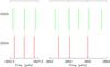Fig. 2 Splittings of the ℓ = 1,ν = 2807.5   μHz (left panel) and ℓ = 2,   ν = 2853.4   μHz (right panel) modes in 2004 and 2005. From Baran et al. (2009).

Telting & Østensen (2006) have published frequencies and line-of-sight velocities based on low-resolution mode spectroscopy acquired during the summer of 2004. Their results are included in Table 2. High-resolution spectroscopy during the summer 2006 was obtained by Telting et al. (2008). They only list the line-of-sight velocity for the fundamental mode: 14.5 km s^-1, which is significantly lower than the 18.9 km s^-1 measured in 2004. In both cases, line-of-sight velocities were computed from cross-correlation profiles (ccp), which merge all spectral lines into a single one, and with a higher signal-to-noise artificial line. Thus, spectral features formed at different depths are combined to produce the ccp’s. Moreover, Balmer lines were used in the low-resolution dataset by Telting & Østensen (2006), while only metallic ones were cross-correlated from the high-resolution data of Telting et al. (2008). Hence, in this case, the change in amplitude can be attributed to the different techniques used.

3. Structure models and non-adiabatic oscillations

3.1. Model 1

For the most part of the work we have considered a single stellar structure model that closely matches the fundamental parameters of Bal09 (Model 1 hereafter). It is a 0.43   M_⊙ total mass model with a hydrogen amount of 2 × 10^-4   M_⊙, T_eff = 26   800 K, and log g = 5.47. Note that the stellar mass equals the seismic mass found by van Grootel et al. (2008). The T_eff and log g are within the observed spectroscopic errors considered by these authors, although we chose T_eff on the low side to ensure unstable g-modes.

The structure model is constructed with a version of the stellar evolution code STARS (Eggleton 1971), updated for asteroseismology. We started the evolution at the ZAEHB, and the particular model we consider is near the end of core He burning with an EHB age of 2.1 × 10⁸ yr. H/He diffusion is included consistently during the evolution, whereas the effects of diffusion of Fe and Ni are approximated with a Gaussian accumulation around log T = 5.3. Radiative opacities that account for the Fe/Ni-enhancement are taken from the Opacity Project (Badnell et al. 2005). More details and input physics are given in Hu et al. (2009) and references therein.

Normal modes of oscillation and eigenfunctions for ℓ ≤ 6 were computed in the linear, non-adiabatic approximation with the pulsation code MAD (Dupret 2001). The structure model was chosen so that the fundamental mode (ν = 2.786   mHz) is close to Balloon’s observed highest amplitude mode at ν = 2.807   mHz. This frequency does not show any rotational splitting and has been identified as a radial mode (Baran et al. 2008; Telting et al. 2008; Charpinet et al. 2008).

In Fig. 3 the Brunt-Väisälä (N) and Lamb (S_ℓ) frequencies for this model are represented. They are displayed in terms of cyclic frequencies so that the propagation cavities are easily delimited in comparison with observed modes. Peaks in N denote gradients in the composition profile, hence, we can distinguish the H envelope (from r/R ~ 0.45 to the surface), the He radiative layer (0.2 ≤ r/R ≤ 0.45) and the inner convective CO core formed as ashes of the He-core burning process. The horizontal lines in the figure correspond to the frequencies of some selected modes: two p-modes at ν = 2807.5 μHz and ν = 2853.4 μHz, which are the ℓ = 1 and ℓ = 2 theoretical counterparts of the observed splittings, and two low-frequency g-modes: ℓ = 4, ν = 436.0   μHz and ℓ = 5, ν = 291.4   μHz.

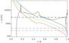Fig. 3 The black solid line is the Brunt-Väisälä frequency, N, while the red, green, blue, and yellow lines are the Lamb acoustic frequencies, Sℓ, for ℓ = 1, 2, 4, and 5, respectively. The dashed horizontal lines correspond to the modes indicated in the text (the ℓ = 1 and ℓ = 2 p-modes look like a single thick line). Model 1 was used.

In the left panel of Fig. 4 we show all computed eigenfrequencies for this structure model, indicating if the mode is linearly unstable (in green) or not (in black). Low-order p-modes (2800 < ν ≲ 4000 μHz) are excited for all angular degrees (ℓ) considered, which can account for the high-frequency peaks detected in Bal09. Another island of unstable modes is due to high-order ℓ > 3 gravity modes. Their frequencies, which are within 400−900 μHz, are slightly shifted compared to the observed low-frequency peaks in Bal09. The relevance of this fact in our work will be discussed below.

The radial and horizontal components of the displacement eigenfunction vector for some particular modes (those indicated in Fig. 3) are included in Fig. 5. The contribution of every point in the star to the dimensionless kinetic energy, ℰ, given by $\mathrm{ℰ}\mathrm{=}\frac{\mathrm{4}\mathit{\pi }{\mathrm{\int }}_{\mathrm{0}}^{\mathit{R}}\mathit{\rho }{\mathit{r}}^{\mathrm{2}}\mathrm{\left[}\mathit{\ell }\mathrm{\right(}\mathit{\ell }\mathrm{+}\mathrm{1}\mathrm{\left)}\mathrm{\right|}{\mathit{\xi }}_{\mathit{h}}{\mathrm{|}}^{\mathrm{2}}\mathrm{+}\mathrm{\left|}{\mathit{\xi }}_{\mathit{r}}{\mathrm{|}}^{\mathrm{2}}\mathrm{\right]}\mathrm{d}\mathit{r}}{\mathit{M}\left[\mathit{\ell }\mathrm{(}\mathit{\ell }\mathrm{+}\mathrm{1}\mathrm{)}\mathrm{\left|}{\mathit{\xi }}_{\mathit{h}}\mathrm{\right(}\mathit{R}\mathrm{)}{\mathrm{|}}^{\mathrm{2}}\mathrm{+}\mathrm{|}{\mathit{\xi }}_{\mathit{r}}\mathrm{\left(}\mathit{R}\mathrm{\right)}{\mathrm{|}}^{\mathrm{2}}\right]}\mathit{,}$(1)is also included in Fig 5. The first two modes on the top are the theoretical eigenfrequencies, which are representative of the observed triplet and quintuplet respectively. The ℓ = 4 and the ℓ = 5 are in the observed g-mode region, albeit only the ℓ = 4 is theoretically unstable.

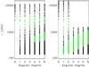Fig. 4 Theoretical eigenfrequencies as function of angular degree. Modes with angular degrees 0 ≤ ℓ ≤ 6 and cyclic frequencies ν > 150   μHz were considered. Excited modes are shown in green. Left panel is for Model 1 and right panel for Model 2.

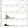Fig. 5 Radial (red, dotted line) and horizontal (green, dot-dashed line) components of the eigenfunctions normalized such that ξr(R) = 1 (p-modes) or ξh(R) = 1 (g-modes), where R is the photospheric radius, for some oscillation modes: from top to bottom: ℓ = 1, ν = 2807.5   μHz, ℓ = 2, ν = 2853.4   μHz, ℓ = 4, ν = 436.0   μHz and ℓ = 5, ν = 291.4   μHz. Also shown (black solid line) is the integrand in the dimensionless kinetic energy ℰ defined by Eq. (1). Model 1 was used.

3.2. Model 2

One of the problems with the current sdB models is that the observed instability strip of the g-modes cannot be correctly modelled. Compared to the observations, typically, the T_eff’s of models with unstable g-modes are too low, the periods of unstable g-modes are too low and only modes with high spherical degree (ℓ ≥ 3) are excited (see e.g. Fontaine et al. 2003; Jeffery & Saio 2006; Hu et al. 2009). This problem is also apparent in our Model 1 as discussed in the previous section. However, Hu et al. (in prep.) have computed new models with atomic diffusion, including radiative levitation of H, He, C, N, O, Ne, Mg, Fe and Ni, that solve the aforementioned problems with the unstable g-modes. Hence, we also compare with such a preliminary model (Model 2 hereafter). Model 2 is obtained from the same ZAEHB model as used for Model 1 but now the evolution and pulsations are computed with fully self-consistent atomic diffusion.

The right panel of Fig. 4 shows the stable and unstable modes for Model 2. In this case there are very many unstable modes in the observed frequency range, between 200   μHz and 800   μHz and including degrees from ℓ = 1 to 6. Note that for higher degrees the frequency range of unstable modes is shifted upwards.

4. Transfer of angular momentum and change in the rotational splitting

Non-radial, non-adiabatic oscillations, especially g-modes with high tangential velocities, can transfer angular momentum to the mean rotational flow. This variation in the rotational velocity will consequently affect the frequency splitting of non-radial g and p-modes.

4.1. Transfer of angular momentum caused by gravity modes

The angular momentum transfer caused by nonaxisymmetric waves in stars can be described in terms of a Reynolds stress (Ando 1981), namely: 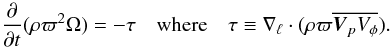$\frac{\mathit{\partial }}{\mathit{\partial t}}\mathrm{\left(}\mathit{\rho }{\mathit{\varpi }}^{\mathrm{2}}\mathrm{\Omega }\mathrm{\right)}\mathrm{=}\mathrm{-}\mathit{\tau } \mathrm{where} \mathit{\tau }\mathrm{\equiv }{\mathrm{\nabla }}_{\mathit{\ell }}\mathrm{·}\mathrm{\left(}\mathit{\rho \varpi }\overline{{V}\mathit{p}{\mathit{V}}_{\mathit{\phi }}}\mathrm{\right)}\mathit{.}$(2)Here ϖ, V_p, V_φ and ∇_ℓ are the cylindrical polar radius, poloidal component of the perturbed velocity, azimuthal component of the perturbed velocity, and poloidal component of the differential operator ∇, respectively. The rotation angular velocity is given by Ω. Here and in the following we will use a similar notation to Unno et al. (1989).

Taking the linear and Cowling approximations in the wave equations, assuming a dependence of the form exp [i(σt + mφ)] , and if the star rotates slowly, such that the real part of the eigenfrequencies obey σ_R ≫ Ω, the change in the angular momentum can be expressed as 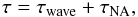$\mathit{\tau }\mathrm{=}{\mathit{\tau }}_{\mathrm{wave}}\mathrm{+}{\mathit{\tau }}_{\mathrm{NA}}\mathit{,}$(3)where the terms τ_wave and τ_NA are given by ${\mathit{\tau }}_{\mathrm{wave}}\mathrm{=}{\mathit{\sigma }}_{\mathrm{R}}{\mathit{\sigma }}_{\mathrm{I}}\mathit{m\rho }\left[\frac{\mathit{\ell }\mathrm{(}\mathit{\ell }\mathrm{+}\mathrm{1}\mathrm{)}\mathrm{|}\mathit{\sigma }{\mathrm{|}}^{\mathrm{2}}}{{\mathit{S}}_{\mathit{\ell }}^{\mathrm{2}}}\mathrm{|}{\mathit{\xi }}_{\mathit{h}}{\mathrm{|}}^{\mathrm{2}}\mathrm{+}\frac{{\mathit{N}}^{\mathrm{2}}}{\mathrm{|}\mathit{\sigma }{\mathrm{|}}^{\mathrm{2}}}\mathrm{|}{\mathit{\xi }}_{\mathit{r}}{\mathrm{|}}^{\mathrm{2}}\right]\mathrm{|}{\mathit{Y}}_{\mathit{\ell }}^{\mathit{m}}{\mathrm{|}}^{\mathrm{2}}$(4)${\mathit{\tau }}_{\mathrm{NA}}\mathrm{=}\frac{\mathrm{1}}{\mathrm{2}}\mathit{mP}\hspace{0.17em}\mathrm{Im}[(\frac{\mathit{\partial P}}{\mathit{P}}{)}^{\mathrm{\ast }}(\frac{\mathit{\partial \rho }}{\mathit{\rho }})]\mathrm{|}{\mathit{Y}}_{\mathit{\ell }}^{\mathit{m}}{\mathrm{|}}^{\mathrm{2}}\mathit{.}$(5)Here σ = σ_R + iσ_I is the complex eigenfrequency of the mode and ${\mathit{Y}}_{\mathit{\ell }}^{\mathit{m}}$ the spherical harmonic. τ_NA represents the transfer of angular momentum through non-adiabatic effects. In this approximation τ_NA is equal to the work function, w(r), except for a constant factor. On the other hand, the term τ_wave represents a wave transience. As explained in Ando (1981), in Eq. (4) for τ_wave, the imaginary part of the eigenfrequency, σ_I, comes from a time derivative of the wave amplitude and hence can be derived appropriately. In particular, it makes sense to take σ_I from the observed changes in the amplitudes of the g-modes, provided they are intrinsic and not caused by beating phenomena.

Figure 6 shows τ_wave and τ_NA as given by Eq. (4) and (5) respectively for an ℓ = 4 unstable mode. According to Eq. (2), these functions give the contribution of each point in the star to the change in the angular momentum. The wave transit term, τ_wave, is similarly weighted as the integrand in the dimensionless energy ℰ (compare to third panel in Fig. 5), while τ_NA, even for inner gravity modes, is only important in the uppermost layers where non- adiabatic effects are significant. The relative importance between both terms depends on the energy of the mode and the value of σ_I considered in τ_wave and will be discussed in the next section.

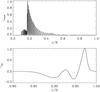Fig. 6 τwave and τNA normalized to the maximum value for a ℓ = 4 g-mode with ν = 436.0   μHz. For τNA only the external layers are shown because it is negligible at deeper ones. Model 1 was used.

Because sdB stars are slowly rotating stars, in principle Eqs. (4) and (5) would be enough for estimating the changes in rotation. However, prograde and retrograde modes contribute in an opposite way to the angular momentum transfer. If modes with the same degree but azimuthal orders  ± m had the same amplitude, the net effect would cancel out. For this reason we will also consider the full expression for τ_NA as given by Eq. (36.16) in Unno et al. (1989): $\begin{array}{ccc}{\mathit{\tau }}_{\mathrm{NAf}}& \mathrm{=}& \mathit{\rho \varpi }\mathrm{Im}\left[{\mathit{v}}_{\mathit{\phi }}^{\mathrm{\ast }}\hspace{0.17em}\mathrm{(}\mathit{\sigma }\mathrm{+}\mathit{m}\mathrm{\Omega }\mathrm{)}{\mathit{v}}_{\mathit{T}}\frac{\mathit{\delta S}}{{\mathit{c}}_{\mathit{p}}}\right]\\ & & \end{array}$(6)where v_p, v_φ and δS are linear perturbations in the poloidal and azimuthal component of the velocity, and the entropy respectively. This equation does not neglect Ω against σ_R nor does it assume the Cowling approximation. However, we shall still consider the eigenfunctions of a non-rotating equilibrium model.

4.2. Effect in the rotational splitting

The rotational splitting, i.e. the perturbation in the frequencies caused by rotation, is given by (e.g. Aerts et al. 2010, Eq. (3.349)) 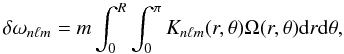$\mathit{\delta }{\mathit{\omega }}_{\mathit{n\ell m}}\mathrm{=}\mathit{m}{\mathrm{\int }}_{\mathrm{0}}^{\mathit{R}}{\mathrm{\int }}_{\mathrm{0}}^{\mathit{\pi }}{\mathit{K}}_{\mathit{n\ell m}}\mathrm{\left(}\mathit{r,\theta }\mathrm{\right)}\mathrm{\Omega }\mathrm{\left(}\mathit{r,\theta }\mathrm{\right)}\mathrm{d}\mathit{r}\mathrm{d}\mathit{\theta ,}$(7)where the kernel K_nℓm(r,θ) is given by $\begin{array}{ccc}{\mathit{K}}_{\mathit{n\ell m}}& \mathrm{=}& [\sin \mathit{\theta }\mathrm{\left\{}\mathrm{\right|}{\mathit{\xi }}_{\mathit{r}}\mathrm{\left(}\mathit{r}\mathrm{\right)}{\mathrm{|}}^{\mathrm{2}}{\mathit{P}}_{\mathit{l}}^{\mathit{m}}\mathrm{(}\mathit{cos\theta }{\mathrm{)}}^{\mathrm{2}}\\ & & \mathrm{+}\mathrm{\left|}{\mathit{\xi }}_{\mathit{h}}\mathrm{\right(}\mathit{r}\mathrm{)}{\mathrm{|}}^{\mathrm{2}}[(\frac{\mathrm{d}{\mathit{P}}_{\mathit{l}}^{\mathit{m}}}{\mathrm{d}\mathit{\theta }}{)}^{\mathrm{2}}\mathrm{+}\frac{{\mathit{m}}^{\mathrm{2}}}{{\sin }^{\mathrm{2}}\mathit{\theta }}{\mathit{P}}_{\mathit{l}}^{\mathit{m}}\mathrm{(}\cos \mathit{\theta }{\mathrm{)}}^{\mathrm{2}}\\ & & \mathrm{-}{\mathit{P}}_{\mathit{l}}^{\mathit{m}}\mathrm{\left(}\mathit{cos\theta }{\mathrm{)}}^{\mathrm{2}}\mathrm{\right[}{\mathit{\xi }}_{\mathit{r}}^{\mathrm{\ast }}\mathrm{\left(}\mathit{r}\mathrm{\right)}{\mathit{\xi }}_{\mathit{h}}\mathrm{\left(}\mathit{r}\mathrm{\right)}\mathrm{+}{\mathit{\xi }}_{\mathit{r}}\mathrm{\left(}\mathit{r}\mathrm{\right)}{\mathit{\xi }}_{\mathit{h}}^{\mathrm{\ast }}\mathrm{\left(}\mathit{r}\mathrm{\right)}\mathrm{]}\\ & & \mathrm{-}\mathrm{2}{\mathit{P}}_{\mathit{l}}^{\mathit{m}}\mathrm{\left(}\mathit{cos\theta }\mathrm{\right)}\frac{\mathrm{d}{\mathit{P}}_{\mathit{l}}^{\mathit{m}}}{\mathrm{d}\mathit{\theta }}\frac{\mathit{cos\theta }}{\sin \mathit{\theta }}\mathrm{\left|}{\mathit{\xi }}_{\mathit{h}}\mathrm{\right(}\mathit{r}\mathrm{\left)}{\mathrm{|}}^{\mathrm{2}}\mathrm{\right\}}]\mathit{\rho }{\mathit{r}}^{\mathrm{2}}\mathit{/}{\mathit{I}}_{\mathit{nlm}}\end{array}$(8)and ${\mathit{I}}_{\mathit{nlm}}\mathrm{=}\frac{\mathrm{2}}{\mathrm{2}\mathit{l}\mathrm{+}\mathrm{1}}\frac{\mathrm{(}\mathit{l}\mathrm{+}\mathrm{|}\mathit{m}\mathrm{\left|}\mathrm{\right)}\mathrm{!}}{\mathrm{(}\mathit{l}\mathrm{-}\mathrm{|}\mathit{m}\mathrm{\left|}\mathrm{\right)}\mathrm{!}}{\mathrm{\int }}_{\mathrm{0}}^{\mathit{R}}[\mathrm{|}{\mathit{\xi }}_{\mathit{r}}{\mathrm{|}}^{\mathrm{2}}\mathrm{+}\mathit{l}\mathrm{(}\mathit{l}\mathrm{+}\mathrm{1}\mathrm{\left)}\mathrm{\right|}{\mathit{\xi }}_{\mathit{h}}{\mathrm{|}}^{\mathrm{2}}]\mathit{\rho }{\mathit{r}}^{\mathrm{2}}\mathrm{d}\mathit{r}\mathit{.}$(9)Therefore, from Eqs. (2) and (7), we obtain the variation of the frequency splitting caused by transfer of angular momentum between eigenmodes and rotation: $\frac{\mathit{\partial }{\mathit{\omega }}_{\mathit{n\ell m}}}{\mathit{\partial t}}\mathrm{=}\mathrm{-}\mathit{m}{\mathrm{\int }}_{\mathrm{0}}^{\mathit{R}}{\mathrm{\int }}_{\mathrm{0}}^{\mathit{\pi }}{\mathit{K}}_{\mathit{n\ell m}}\mathrm{\left(}\mathit{r,\theta }\mathrm{\right)}\frac{{\mathit{\tau }}_{{\mathit{n}}^{\mathrm{\prime }}{\mathit{l}}^{\mathrm{\prime }}{\mathit{m}}^{\mathrm{\prime }}}}{\mathit{\rho }{\mathit{r}}^{\mathrm{2}}{\sin }^{\mathrm{2}}\mathit{\theta }}\mathrm{d}\mathit{r}\mathrm{d}\mathit{\theta ,}$(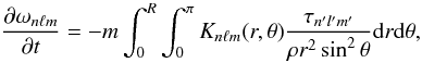10)where n, ℓ, and m are for the mode for which the rotational splitting is considered and n′, ℓ′, m′ are for the mode for which the transfer of angular momentum is computed.

Figure 7 shows the normalized outcome of Eq. (10) when either the wave transit term τ_wave (top panel) or the non-adiabatic term τ_NA (bottom panel) are considered. Here we have chosen the splitting of the theoretical ℓ = 1 p-mode closest in frequency to the observed triplet and computed the change caused by a single, unstable, ℓ = 4 g-mode. For τ_wave, the change in the splitting is mainly caused in the external layers, whereas the angular momentum transfer takes place in deeper regions, see Fig. 6. This is a straightforward consequence of the nature of the p-mode considered for measuring the rotational splitting that have higher amplitudes in the external layers. For τ_NA the external layers are dominant for both the rotational splitting variation and the angular momentum transfer, although the weights are different.

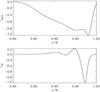Fig. 7 Contribution of the different layers to the change in the splitting of the l = 1, ν = 2807.5   μHz mode due to the ℓ = 4, m = 4, ν = 436   μHz g-mode according to Eq. (10). Top panel is for τwave and bottom panel for τNA. Values were normalized to the maximum. Note that only the upper layers of the model are shown because the contribution of deeper layers is negligible. Model 1 was used.

4.3. Visibility

Because all computations are based on the linear theory, the eigenfunctions are calculated except for a constant factor that can be fixed by, for example, the velocity amplitude at a given point in the atmosphere. In principle velocity observations are easier, less model-dependent, and more related to theoretical values than photometric observations, and therefore we will use them. However, as commented in Sect. 2, the line-of-sight-velocity observations do not correspond to a specific point in the atmosphere. Because the amplitude of the modes change by more than one order of magnitude throughout the atmosphere, an accurate determination would require a detailed theoretical simulation of the observational measurements. In this work we will perform a simple calibration between observed and theoretical amplitudes by assuming that the observations correspond to a unique optical depth, τ_R, but considering different values.

Specifically, we use a relation between the amplitude of the radial component of the velocity, v_p, and the observed line-of-sight velocity, v_obs. The proportionality factor, which we will call the visibility, A(ℓ,m,ω), is given by ${\mathit{v}}_{\mathrm{obs}}\mathrm{=}\mathit{A}\mathrm{\left(}\mathit{\ell ,m,\omega }\mathrm{\right)}\hspace{0.17em}{\mathit{v}}_{\mathit{p}} \mathrm{attheobservedpoint}\mathrm{.}$(11)Given that we observe v_obs for certain modes, we can retrieve their v_p if we are able to compute A(ℓ,m,ω). The factor A(ℓ,m,ω) includes the geometrical effects of the velocity projection as well as limb-darkening effects. It also depends on the inclination angle i and the ratio between the horizontal and vertical components of the eigenfunctions, K = ξ_h/ξ_r at the observed point. To avoid the dependence on i, the rms value over m can be used. When referring to this average, we will just remove the m dependence, A(ℓ,ω).

To compute A(ℓ,m,ω) we have mostly followed the formalism in Aerts et al. (1992). However, in that work the approximation $\mathit{K}\mathrm{\approx }\mathrm{\left(}\mathit{GM}\mathrm{\right)}\mathit{/}\mathrm{\left(}{\mathit{R}}^{\mathrm{3}}{\mathit{\sigma }}^{\mathrm{2}}\mathrm{\right)}$(12)was used. This approximation is derived by assuming a Lagrangian pressure perturbation at the outer boundary of δP = 0, which is valid for adiabatic oscillations, provided that the boundary condition is not located too deep in the atmosphere. However, Eq. (12) is not valid if non-adiabatic effects are important. Because we have computed the theoretical eigenfunctions in a non-adiabatic approximation for our specific models, we can compute the precise ratio K at the required point in the atmosphere.

In Fig. 8 we show the K ratio evaluated at two optical depths. The approximate K from Eq. (12) is also included for comparison. Note that the approximation agrees better with the actual theoretical values at higher depths, where non-adiabatic effects are less important. The visibility factors A(ℓ,ω) depend on the optical depth through limb-darkening coefficients and the ratio K, which is negligible for p-modes. However, for g-modes it can be as large as 100 or 1000 (as can be seen in Fig. 8) and as a result g-modes can have rather different visibility factors depending on the optical depth considered.

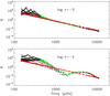Fig. 8 K ratio between horizontal and radial components of the displacement vector at optical depths log τR =  −3 and log τR =  −4. Black points include all linearly stable modes while green points are for the unstable ones (Model 1). Red crosses are the ratios expected by the approximate Eq. (12).

Because the horizontal components of the g-modes are very large, the visibility factors as defined by Eq. (11) are not by themselves indicative of the kind of modes we expect to observe. It is more illustrative to express the visibility in terms of the energy of the modes. The kinetic energy, averaged over time, can be expressed as (see e.g. Aerts et al. 2010) 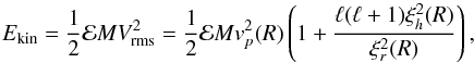${\mathit{E}}_{\mathrm{kin}}\mathrm{=}\frac{\mathrm{1}}{\mathrm{2}}\mathrm{ℰ}\mathit{M}{\mathit{V}}_{\mathrm{rms}}^{\mathrm{2}}\mathrm{=}\frac{\mathrm{1}}{\mathrm{2}}\mathrm{ℰ}\mathit{M}{\mathit{v}}_{\mathit{p}}^{\mathrm{2}}\mathrm{\left(}\mathit{R}\mathrm{\right)}\left(\mathrm{1}\mathrm{+}\frac{\mathit{\ell }\mathrm{(}\mathit{\ell }\mathrm{+}\mathrm{1}\mathrm{)}{\mathit{\xi }}_{\mathit{h}}^{\mathrm{2}}\mathrm{\left(}\mathit{R}\mathrm{\right)}}{{\mathit{\xi }}_{\mathit{r}}^{\mathrm{2}}\mathrm{\left(}\mathit{R}\mathrm{\right)}}\right)\mathit{,}$(13)where ℰ is given by Eq. (1), V_rms is the root mean-squared velocity over the stellar surface, at radius R and M is the total mass of the star. Using Eqs. (13) and (11) we obtain the following relation between the line-of-sight velocity and the kinetic energy of the modes: 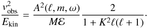$\frac{{\mathit{v}}_{\mathrm{obs}}^{\mathrm{2}}}{{\mathit{E}}_{\mathrm{kin}}}\mathrm{=}\frac{{\mathit{A}}^{\mathrm{2}}\mathrm{\left(}\mathit{\ell ,m,\omega }\mathrm{\right)}}{\mathit{M}\mathrm{ℰ}}\frac{\mathrm{2}}{\mathrm{1}\mathrm{+}{\mathit{K}}^{\mathrm{2}}\mathit{\ell }\mathrm{(}\mathit{\ell }\mathrm{+}\mathrm{1}\mathrm{)}}\mathrm{·}$(14)The right-hand side of Eq. (14) can be theoretically computed, and it is shown in Fig. 9 for two different optical depths. They were normalized to the fundamental mode. Note that g-modes in the observed frequency range have much higher values than the fundamental one and hence need much less excitation energy to be observed with similar Doppler velocities. This is true not only for the lowest degrees but also for ℓ = 4 and ℓ = 5. Moreover, this conclusion is valid for any optical depth in the range considered.

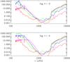Fig. 9 Ratio $\mathrm{\left|}{\mathit{v}}_{\mathrm{obs}}\mathrm{\right|}\mathit{/}\sqrt{{\mathit{E}}_{\mathrm{kin}}}$ normalized to the fundamental mode. See text and Eq. (14) for an explanation. Modes with the same degree were joined for clarity. Black, red, green, blue, yellow and magenta correspond to angular degrees ℓ = 0, 1, 2, 3, 4, and 5, respectively. Upper panel is for log τR =  −3 and bottom panel is for log τR =  −4.

4.4. Amplitude calibration

According to Eqs. (3)–(5) and (10) the transfer of angular momentum and the change in the splittings are proportional to the eigenfrequency squares and hence the amplitude square of the g-modes considered. Because the amplitude of the modes can increase by an order of magnitude throughout the atmosphere, a very important question concerning Eq. (11) is where to fix the point where observed velocities are transformed into theoretical ones. Following Rauch et al. (2010), the formation depth of the core of the Balmer lines in the subdwarf stars seems to be at optical depths between τ_R ≃ 0.1 and τ_R ≳ 0.01. However, the wings of the lines are formed higher in the atmosphere and because the amplitude of the modes increase with height, the oscillatory signal could come from optical depths substantially lower than that of the core. Here we shall try not to overestimate the change in the angular momentum caused by the oscillations. Therefore we assumed the g-mode energies to be as small as possible, and located the signal as high as possible in the atmosphere. We will take τ_R = 0.001 as a reference value.

Because only few g-modes are observed in velocity and they cannot be identified (l and m are unknown), we need some hypothesis about the excitation energy to be able to proceed. To calibrate the theoretical amplitudes we attribute a line-of-sight velocity of v_obs = 1   km s^-1 to the g-mode with the highest ${\mathit{v}}_{\mathrm{obs}}^{\mathrm{2}}\mathit{/}{\mathit{E}}_{\mathrm{kin}}$ in the frequency range  [250,400]    μHz. The value of v_obs and the frequency range considered are based on the observations. Our choice gives the minimum energy required to reproduce the observational amplitudes in the g-mode region. At the two optical depths considered in Fig. 8, the theoretical mode that matches this requirement is a ℓ = 3, ν = 276   μHz eigenmode for Model 1. but there are other l = 2,...,5 modes that if taken as representative of the observations would result in a similar E_kin, so the particular mode is not important for an order of magnitude estimation.

On the other hand, the optical depth of the model at which the line-of-sight velocity is calibrated has a large impact on the results. For the above g-mode, the amplitude of the radial velocity eigenfunction at an optical depth of log τ_R =  −3 is 5.3 times smaller than that at log τ_R =  −4. Because the change in the splitting is proportional to the velocity square, a factor of 28 difference is found between both optical depths.

5. Results

In the following computations we assume the same kinetic energy for all modes, although there is no particular theoretical reason for this. However, from the velocity observations, we known that at least a few modes in the frequency range  [250,400]    μHz need to have an E_kin this large and the observations in photometry reveal that indeed several g-modes are excited to similar amplitudes and hence, perhaps, energies. On the other hand, if E_kin varies in orders of magnitude with frequency or angular degree, the actual behaviour of the changes in the rotational splittings, proportional to E_kin, can be very different from those shown in the following figures. Therefore, we can estimate the order of magnitude of the change from individual modes but we are not able to compute a net effect from the entire g-modes.

5.1. The non-adiabatic term, τ_NA

Let us start by considering the changes in the splitting due to the non-adiabatic term τ_NA of individual g-modes with m > 0. In Fig. 10 we show the change in the splitting of the ℓ = 1, ν = 2807   μHz mode owing to g-modes with ℓ = 4, m = 4. Equation (5) for τ_NA using Model 1. In the figure, the energy E_kin was fixed by taking the value v_obs = 1   km s^-1 at log τ_R =  −3 for the reference mode given in Sect. 4.4. The modes that induce the most significant changes in the splitting are in the observed frequency range, although most of them are not expected to be excited in Model 1. It follows from Fig. 10 that the change in the splitting of the theoretical counterpart of the observed triplet is as large as 0.02   μHz/yr if log τ_R =  −3 is assumed, considering only the contribution of the ℓ = 4, m = 4 g-modes. Slightly higher values are obtained if ℓ = 5, m = 5 g-modes are considered. These changes for single modes are only an order of magnitude smaller than the observed values. On the other hand, as stated before, calibrating the observed amplitude at an optical depth of log τ_R =  −4 results in changes in the rotational splittings of about 28 times smaller. Thus the resulting splitting for the same single modes would be about 0.007   μHz/yr.

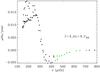Fig. 10 Change in the rotational splitting of the ℓ = 1, ν = 2807.5   μHz p-mode owing to the ℓ = 4, m = 4 g-modes, considering the τNA term. Here we assume the same energy for all modes and fix it so that vobs = 1   km s-1 for ℓ = 3,ν = 276   μHz at log τR =  −3. Black points are for stable modes and green points for the unstable ones. Model 1 was used.

However, the net effect could be much lower because modes with the same degree ℓ and radial order n but different azimuthal orders m can be expected to be excited to very similar amplitudes and, according to Eq. (5), the change in the rotation through  ± m pairs would mostly cancel out. Note also that high-frequency g-modes give a contribution opposite to that of low-frequency g-modes, as seen in Fig. 10.

To examine the possible reduction of the net effect, we now assume the same amplitude for all 2ℓ + 1 azimuthal modes with the same angular degree ℓ and radial order n and use the full expression of τ_NAf (Eq. (6)) to compute the change in splitting. Fig. 11 shows the changes in the splitting of the same ℓ = 1, ν = 2807.5   μHz p-mode owing to the ℓ = 4, g-modes. The energy of the modes were again fixed by assuming an optical depth of log τ_R =  −3. In this case the change induced by isolated (2ℓ + 1) group of modes can be as large as 0.004   μHz/year, which is 60 times smaller than the observed one. Again, considering the ℓ = 5 modes, slightly higher values are obtained while for log τ_R =  −4 the effect will be reduced by a factor 28.

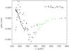Fig. 11 Change in the rotational splitting of the ℓ = 1, ν = 2807.5   μHz p-mode owing to ℓ = 4 multiplets, assuming the same amplitude for all modes with different m but the same ℓ,n numbers, and considering the τNAf term. As before we assume the same energy for all modes and fix it so that the ℓ = 3,ν = 276   μHz mode would have an observed velocity vobs = 1   km s-1 if it were to be observed at an optical depth log τR =  −3. Model 1 has been used.

Sumning the contribution of all modes would probably increase the change in rotational splitting to even higher values than we give here. However, as explained at the beginning of Sect. 5, we do not find it realistic to give a conclusive summed-up number. Instead, our results should be considered as a low order of magnitude estimate of the change in rotational splitting caused by angular momentum transfer.

5.2. The transient term τ_wave

Here we consider the changes induced by the term τ_wave. This term is caused by a change in the mode amplitude, represented in Eq. (4) by the term σ_I. Because the eigenfrequencies are computed in the linear theory, considering the theoretical values σ_I serves no purpose. On the other hand, as shown in Table 1, the mode amplitude is changing yearly between campaigns. These changes can be caused by different factors, such as beating phenomena, but as an upper limit we can assume they are completely caused by intrinsic changes in the mode amplitudes. A value of σ_I = 1/year is consistent with the results in Table 1. In any case, because the change in the splittings are proportional to σ_I the results are easly transformed into other amplitude variations. Figure 12 shows the results in the splitting of the ℓ = 1, ν = 2807.5   μHz p-mode owing to the ℓ = 4, m = 4 g-modes. Compared to Fig. 10 we see that this changes are about 100 times smaller than those corresponding to τ_NA. Thus, unless the changes in the mode amplitudes have time scales much shorter than a year, the contribution of τ_wave can be neglected as compared to the τ_NA effect.

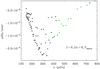Fig. 12 Change in the rotational splitting of the ℓ = 1, ν = 2807.5   μHz p-mode owing to the ℓ = 4, m = 4 g-modes considering the τwave term. Here we assume the same energy for all modes and fix it so that vobs = 1   km s-1 for ℓ = 3, ν = 276   μHz at log τR =  −3. Black points are for stable modes and green points for the unstable ones. Model 1 was used.

5.3. Changes in the splitting for different modes

So far we have limited the computations to the changes in the observed triplet (assuming a ℓ = 1, low-order p-mode). However, the change in the splitting strongly depends on the frequency of the p or g-mode used as the test. On the other hand, the expected change for the ℓ = 2 modes are very similar to that of the ℓ = 1 when compared at a given frequency, except for a factor m for p-modes and a factor m { 1 − 1/ [l(l + 1)]  }  for g-modes, both well known results from the asymptotic theory. To illustrate the frequency dependence, Fig. 13 shows the changes in all ℓ = 1 modes owing to a g-mode with ℓ = 4,ν ~ 300   μHz. From Fig. 13 follows that the most pronounced changes are expected for p-modes with high radial order. The observed triplet is around 2800   μHz but higher p-modes are in fact observed. So this result is potentially very interesting because we predict changes in the splitting around or above 1   μHz/year. Also, the change in the rotational splitting of low-frequency g-modes would be significantly larger than those corresponding to the observed modes, but measuring rotational splitting in this region could be a difficult task because of the large population of peaks and beating phenomena in the signal.

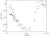Fig. 13 Change in the rotational splittings of the ℓ = 1,m = 1 modes owing to the and ℓ = 4, m = 4, ν ≃ 300   μHz mode. Absolute values were considered. The energy of the mode was fixed in a way that vobs = 1   km s-1 for ℓ = 3, ν = 276   μHz at log τR =  −3 for Model 1. Black point are for Model 1 and red points for Model 2. The g-mode considered has ν = 305.14   μHz in Model 1 and ν = 301.02   μHz in Model 2.

Because τ_NA is proportional to the work function, the change in the splittings is determined by the same non-adiabatic properties of the g-mode eigenfunctions as the growth rates, although the integrals over the whole star have different weights. Because the modes with the largest contribution to the changes in the rotational splittings are stable in Model 1, this can be an important source of errors. On the other hand, as shown in Fig. 4, g-modes with l ≤ 5 and low frequencies are unstable in Model 2 and hence, in principle, using this new model would avoid that problem. Fig. 13 allows to analyse this problem. The g-mode chosen for the transfer of angular momentum is expected to be stable if Model 1 is used and unstable if Model 2 is used. Despite this fact, Fig. 13 shows that the results for both models are fairly similar, or a little higher for Model 2, if compared at the same frequency of the test mode. This allows us to be confident in the results obtained with Model 1. The reason for using Model 1 in the previous figures was that the frequencies of the l = 1 and l = 2 lowest p-modes are very close to the observed triplet and quintuplet while, as previously mentioned, we do not yet have a model with the new physics that accurately match the observed p-modes.

6. Conclusions

Transfer of angular momentum between g-modes and rotation can explain the changes in the rotational splittings observed in the sdB star Balloon 090100001. We performed the computations by estimating the mode energies from the observed g-mode velocities and using structure models that fit the stellar parameters, including the frequencies of the highest amplitude p-modes. The theoretical changes found for the rotational splittings caused by single g-modes are about one order of magnitude smaller than the observed ones if an optical depth of log τ_R =  −3 is considered for the calibration. If the cancellation effect between prograde and retrograde modes are considered by assuming the same amplitude for the rotational multiplets, the net effect is about 60 times lower than the observed ones. Because the optical depth considered is rather a lower limit and because the observed value should be compared with the net effect from all g-modes, we can conclude that this mechanism can produce a rotational splitting of the same order of magnitude as the observed ones. Moreover, we find that the transfer of angular momentum is possible because of the non-adiabatic nature of high radial order, low-degree g-modes, even if the amplitude of the modes do not vary. Indeed, changes in the amplitudes within a yearly time scale, as it seems to be the case in this and other sdB stars, induce a much smaller change in the rotational splittings than the non-adiabatic process.

Although Ba09 has brought us an opportunity for checking this kind of stellar phenomena, some uncertainties prevent us from obtaining more quantitative results. One uncertainty comes from performing an accurate calibration between observed velocities and theoretical energies, because the former cannot be easily translated into values at a specific optical depth or to a some weighted integral over the atmosphere. Photometric observations can help here, but a calibration of these observations are generally more complex and model-dependent than the velocity ones because changes in the flux are caused by non-adiabatic effects. This problem could be limited in the future by performing detailed theoretical simulations of the data analysis.

A second problem that hinders more quantitative calculations concerns the mode identification in the low-frequency range. But even if this were possible, the main contribution to the transfer of angular momentum can come from high-degree modes that are not observed owing to geometrical cancellations. However, it is interesting to note that potentially observed modes and modes contributing the most to the changes in the rotational splitting can be quite close in frequency and degree. As can be seen in Fig. 4, Model 2 predicts unstable modes with a frequency range that resembles the observed one. There are unstable modes for all angular degrees considered, but for higher degrees the unstable modes shift towards higher frequencies. Thus the main contribution that according to Figs. 10 and 11 appears for frequencies below 400 or 500   μHz could come from modes of degrees in the observed range or at most a little higher, say ℓ ≤ 5 or 6.

According to Eq. (2), because τ depends on latitude, so does the change on the rotational velocity. Hence, g-modes induce a differential rotation in the stars. It is interesting to note that the quintuplet did show a latitudinally differential rotation, and therefore the same angular momentum transfer can be invoked as the cause for the differential rotation.

Searching for other sdB stars with similar characteristics would allow us to improve our knowledge. This involves in particular space missions like COROT and KEPLER (Borucki et al. 2010) that can acquire high-precision and long-term photometry of pulsating hot subdwarfs, which is of utmost importance to detect the possible effects in frequency splittings caused by angular momentum transfer. However, there is only one p-mode pulsator identified in the FoV of Kepler (Kawaler et al. 2010) and a handful of g-mode pulsating sdBs with candidate splitting patterns that still need longer time series to be confirmed (Østensen et al. 2010, 2011).

Acknowledgments

Part of this work was supported by the Spanish National Research Plan under project AYA2010-17803. H.H. is supported by a Rubicon fellowship of the Netherlands Organisation for Scientific Research (NWO).

References

All Tables

All Figures

	Fig. 1 Comparison of the amplitude spectrum of Bal09 in 2004 and 2005 after removing the three highest peaks. Figure from Baran et al. (2009). P, g, and c stand for p-modes, g-modes, and combination frequencies, respectively.
In the text

	Fig. 2 Splittings of the ℓ = 1,ν = 2807.5   μHz (left panel) and ℓ = 2,   ν = 2853.4   μHz (right panel) modes in 2004 and 2005. From Baran et al. (2009).
In the text

	Fig. 3 The black solid line is the Brunt-Väisälä frequency, N, while the red, green, blue, and yellow lines are the Lamb acoustic frequencies, Sℓ, for ℓ = 1, 2, 4, and 5, respectively. The dashed horizontal lines correspond to the modes indicated in the text (the ℓ = 1 and ℓ = 2 p-modes look like a single thick line). Model 1 was used.
In the text

	Fig. 4 Theoretical eigenfrequencies as function of angular degree. Modes with angular degrees 0 ≤ ℓ ≤ 6 and cyclic frequencies ν > 150   μHz were considered. Excited modes are shown in green. Left panel is for Model 1 and right panel for Model 2.
In the text

Fig. 5 Radial (red, dotted line) and horizontal (green, dot-dashed line) components of the eigenfunctions normalized such that ξr(R) = 1 (p-modes) or ξh(R) = 1 (g-modes), where R is the photospheric radius, for some oscillation modes: from top to bottom: ℓ = 1, ν = 2807.5   μHz, ℓ = 2, ν = 2853.4   μHz, ℓ = 4, ν = 436.0   μHz and ℓ = 5, ν = 291.4   μHz. Also shown (black solid line) is the integrand in the dimensionless kinetic energy ℰ defined by Eq. (1). Model 1 was used.

In the text

	Fig. 6 τwave and τNA normalized to the maximum value for a ℓ = 4 g-mode with ν = 436.0   μHz. For τNA only the external layers are shown because it is negligible at deeper ones. Model 1 was used.
In the text

	Fig. 7 Contribution of the different layers to the change in the splitting of the l = 1, ν = 2807.5   μHz mode due to the ℓ = 4, m = 4, ν = 436   μHz g-mode according to Eq. (10). Top panel is for τwave and bottom panel for τNA. Values were normalized to the maximum. Note that only the upper layers of the model are shown because the contribution of deeper layers is negligible. Model 1 was used.
In the text

	Fig. 8 K ratio between horizontal and radial components of the displacement vector at optical depths log τR =  −3 and log τR =  −4. Black points include all linearly stable modes while green points are for the unstable ones (Model 1). Red crosses are the ratios expected by the approximate Eq. (12).
In the text

Fig. 9 Ratio $\mathrm{\left|}{\mathit{v}}_{\mathrm{obs}}\mathrm{\right|}\mathit{/}\sqrt{{\mathit{E}}_{\mathrm{kin}}}$ normalized to the fundamental mode. See text and Eq. (14) for an explanation. Modes with the same degree were joined for clarity. Black, red, green, blue, yellow and magenta correspond to angular degrees ℓ = 0, 1, 2, 3, 4, and 5, respectively. Upper panel is for log τR =  −3 and bottom panel is for log τR =  −4.

In the text

	Fig. 10 Change in the rotational splitting of the ℓ = 1, ν = 2807.5   μHz p-mode owing to the ℓ = 4, m = 4 g-modes, considering the τNA term. Here we assume the same energy for all modes and fix it so that vobs = 1   km s-1 for ℓ = 3,ν = 276   μHz at log τR =  −3. Black points are for stable modes and green points for the unstable ones. Model 1 was used.
In the text

Fig. 11 Change in the rotational splitting of the ℓ = 1, ν = 2807.5   μHz p-mode owing to ℓ = 4 multiplets, assuming the same amplitude for all modes with different m but the same ℓ,n numbers, and considering the τNAf term. As before we assume the same energy for all modes and fix it so that the ℓ = 3,ν = 276   μHz mode would have an observed velocity vobs = 1   km s-1 if it were to be observed at an optical depth log τR =  −3. Model 1 has been used.

In the text

	Fig. 12 Change in the rotational splitting of the ℓ = 1, ν = 2807.5   μHz p-mode owing to the ℓ = 4, m = 4 g-modes considering the τwave term. Here we assume the same energy for all modes and fix it so that vobs = 1   km s-1 for ℓ = 3, ν = 276   μHz at log τR =  −3. Black points are for stable modes and green points for the unstable ones. Model 1 was used.
In the text

Fig. 13 Change in the rotational splittings of the ℓ = 1,m = 1 modes owing to the and ℓ = 4, m = 4, ν ≃ 300   μHz mode. Absolute values were considered. The energy of the mode was fixed in a way that vobs = 1   km s-1 for ℓ = 3, ν = 276   μHz at log τR =  −3 for Model 1. Black point are for Model 1 and red points for Model 2. The g-mode considered has ν = 305.14   μHz in Model 1 and ν = 301.02   μHz in Model 2.

In the text

References

- Aerts, C., de Pauw, M., & Waelkens, C. 1992, A&A, 266, 294 [NASA ADS] [Google Scholar]
- Aerts, C., Christensen-Dalsgaard, J., & Kurtz, D. W. 2010, Asteroseismology (Heidelberg, Springer) [Google Scholar]
- Ando, H. 1981, MNRAS, 197, 1139 [NASA ADS] [Google Scholar]
- Ando, H. 1983, PASJ, 35, 343 [Google Scholar]
- Badnell, N. R., Bautista, M. A., Butler, K., et al. 2005, MNRAS, 360, 458 [NASA ADS] [CrossRef] [Google Scholar]
- Baran, A., Pigulski, A., & O’Toole, S. J. 2008, MNRAS, 385, 255 [NASA ADS] [CrossRef] [Google Scholar]
- Baran, A., Oreiro, R., Pigulski, A., et al. 2009, MNRAS, 392, 1092 [NASA ADS] [CrossRef] [Google Scholar]
- Baran, A. S., Gilker, J. T., Fox-Machado, L., Reed, M. D., & Kawaler, S. D. 2011, MNRAS, 411, 776 [NASA ADS] [CrossRef] [Google Scholar]
- Borucki, W. J., Koch, D., Basri, G., et al. 2010, Science, 327, 977 [NASA ADS] [CrossRef] [PubMed] [Google Scholar]
- Charpinet, S., Fontaine, G., Brassard, P., et al. 1997, ApJ, 483, L123 [NASA ADS] [CrossRef] [PubMed] [Google Scholar]
- Charpinet, S., Fontaine, G., Brassard, P., et al. 2008, in Hot Subdwarf Stars and Related Objects, ed. U. Heber, C. S. Jeffery, & R. Napiwotzki, (San Francisco: ASP), 392, 297 [Google Scholar]
- D’Cruz, N. L., Dorman, B., Rood, R. T., & O’Connell, R. W. 1996, ApJ, 466, 359 [NASA ADS] [CrossRef] [Google Scholar]
- Dorman, B., Rood, R. T., & O’Connell, R. W. 1993, ApJ, 419, 596 [CrossRef] [Google Scholar]
- Dupret, M. A. 2001, A&A, 366, 166 [NASA ADS] [CrossRef] [EDP Sciences] [Google Scholar]
- Eggleton, P. P. 1971, MNRAS, 151, 351 [NASA ADS] [CrossRef] [Google Scholar]
- Fontaine, G., Brassard, P., Charpinet, S., et al. 2003, ApJ, 597, 518 [Google Scholar]
- Geier, S., Heber, U., Kupfer, T., & Napiwotzki, R. 2010, A&A, 515, A37 [NASA ADS] [CrossRef] [EDP Sciences] [Google Scholar]
- Green, E. M., Fontaine, G., Reed, M. D., et al. 2003, ApJ, 583, L31 [NASA ADS] [CrossRef] [Google Scholar]
- Heber, U. 1986, A&A, 155, 33 [NASA ADS] [Google Scholar]
- Hu, H., Dupret, M., Aerts, C., et al. 2008, A&A, 490, 243 [NASA ADS] [CrossRef] [EDP Sciences] [Google Scholar]
- Hu, H., Nelemans, G., Aerts, C., & Dupret, M.-A. 2009, A&A, 508, 869 [NASA ADS] [CrossRef] [EDP Sciences] [Google Scholar]
- Jeffery, C. S., & Saio, H. 2006, MNRAS, 371, 659 [NASA ADS] [CrossRef] [Google Scholar]
- Kawaler, S. D., Reed, M. D., Quint, A. C., et al. 2010, MNRAS, 409, 1487 [NASA ADS] [CrossRef] [Google Scholar]
- Kilkenny, D. 2010, Ap&SS, 329, 175 [NASA ADS] [CrossRef] [Google Scholar]
- Kilkenny, D., Koen, C., O’Donoghue, D., & Stobie, R. S. 1997, MNRAS, 285, 640 [Google Scholar]
- Kumar, P., Talon, S., & Zahn, J. 1999, ApJ, 520, 859 [NASA ADS] [CrossRef] [Google Scholar]
- Lutz, R., Schuh, S., Silvotti, R., et al. 2009, A&A, 496, 469 [NASA ADS] [CrossRef] [EDP Sciences] [Google Scholar]
- Moni Bidin, C., Villanova, S., Piotto, G., & Momany, Y. 2011, A&A, 528, A127 [NASA ADS] [CrossRef] [EDP Sciences] [Google Scholar]
- Oreiro, R., Ulla, A., Pérez Hernández, F., et al. 2004, A&A, 418, 243 [NASA ADS] [CrossRef] [EDP Sciences] [Google Scholar]
- Oreiro, R., Pérez Hernández, F., Ulla, A., et al. 2005, A&A, 438, 257 [NASA ADS] [CrossRef] [EDP Sciences] [Google Scholar]
- Østensen, R. H., Silvotti, R., Charpinet, S., et al. 2010, MNRAS, 409, 1470 [NASA ADS] [CrossRef] [Google Scholar]
- Østensen, R. H., Silvotti, R., Charpinet, S., et al. 2011, MNRAS, 414, 2860 [NASA ADS] [CrossRef] [Google Scholar]
- Rauch, T., Werner, K., & Kruk, J. W. 2010, Ap&SS, 329, 133 [NASA ADS] [CrossRef] [Google Scholar]
- Schuh, S., Huber, J., Dreizler, S., et al. 2006, A&A, 445, L31 [NASA ADS] [CrossRef] [EDP Sciences] [Google Scholar]
- Talon, S., Kumar, P., & Zahn, J. 2002, ApJ, 574, L175 [NASA ADS] [CrossRef] [Google Scholar]
- Telting, J. H., & Østensen, R. H. 2006, A&A, 450, 1149 [NASA ADS] [CrossRef] [EDP Sciences] [Google Scholar]
- Telting, J. H., Geier, S., Østensen, R. H., et al. 2008, A&A, 492, 815 [NASA ADS] [CrossRef] [EDP Sciences] [Google Scholar]
- Unno, W., Osaki, Y., Ando, H., Saio, H., & Shibahashi, H. 1989, Nonradial oscillations of stars, ed. W. Unno, Y. Osaki, H. Ando, H. Saio, & H. Shibahashi (Tokyo: University of Tokyo press) [Google Scholar]
- van Grootel, V., Charpinet, S., Fontaine, G., et al. 2008, A&A, 488, 685 [NASA ADS] [CrossRef] [EDP Sciences] [Google Scholar]
- Zahn, J., Talon, S., & Matias, J. 1997, A&A, 322, 320 [NASA ADS] [Google Scholar]
All Tables
Frequency analysis based on low-resolution spectroscopy by Telting & Østensen (2006).