| Issue |
A&A
Volume 534, October 2011
|
|
|---|---|---|
| Article Number | A56 | |
| Number of page(s) | 12 | |
| Section | Extragalactic astronomy | |
| DOI | https://doi.org/10.1051/0004-6361/201117533 | |
| Published online | 03 October 2011 | |
Dense gas in nearby galaxies
XVII. The distribution of ammonia in NGC 253, Maffei 2, and IC 342⋆
1
Department of Physical Sciences, University of Puerto Rico, PO Box 23323, 00931-3323 San Juan, Puerto Rico
2
Max-Planck-Institut für Radioastronomie, Auf dem Hügel 69, 53121 Bonn, Germany
3
National Radio Astronomy Observatory, 520 Edgemont Road, VA 22903 Charlottesville, USA
e-mail: jmangum@nrao.edu
4
Joint ALMA Observatory, Av. Alonso de Córdova 3107, Vitacura, Santiago, Chile
5
Instituto de Radioastronomía Milimétrica, Avda. Divina Pastora 7, Local 20, 18012 Granada, Spain
6
Astronomy Department, Faculty of Science, King Abdulaziz University, PO Box 80203, Jeddah, Saudi Arabia
7 INAF-Osservatorio Astronomico di Cagliari, Loc. Poggio dei Pini, Strada 54, 09012 Capoterra (CA), Italy
Received: 21 June 2011
Accepted: 24 August 2011
Context. The central few 100 pc of galaxies often contain large amounts of molecular gas. The chemical and physical properties of these extragalactic star formation regions differ from those in galactic disks, but are poorly constrained.
Aims. This study aims to develop a better knowledge of the spatial distribution and kinetic temperature of the dense neutral gas associated with the nuclear regions of three prototypical spiral galaxies, NGC 253, IC 342, and Maffei 2.
Methods. VLA CnD and D configuration measurements have been made of three ammonia (NH3) inversion transitions.
Results. The (J,K) = (1, 1) and (2, 2) transitions of NH3 were imaged toward IC 342 and Maffei 2. The (3, 3) transition was imaged toward NGC 253. The entire flux obtained from single-antenna measurements is recovered for all three galaxies observed. Derived lower limits to the kinetic temperatures determined for the giant molecular clouds in the centers of these galaxies are between 25 and 50 K. There is good agreement between the distributions of NH3 and other H2 tracers, such as rare CO isotopologues or HCN, suggesting that NH3 is representative of the distribution of dense gas. The “Western Peak” in IC 342 is seen in the (6, 6) line but not in lower transitions, suggesting maser emission in the (6, 6) transition.
Key words: galaxies: ISM / galaxies: abundances / galaxies: starburst / radio lines: galaxies / galaxies: general
Appendix A is available in electronic form at http://www.aanda.org
© ESO, 2011
1. Introduction
A large fraction (~20% at z < 0.2, Brinchmann et al. 2004) of all stars, and as a consequence many of the massive stars in our Universe, are being born in the central regions of starburst galaxies. The reservoirs for such starbursts are large concentrations of dense molecular gas, which in many cases are formed by the interaction of two or more galaxies, which triggers the infall of large quantities of material toward the central few hundred parsecs in these systems (Combes 2005). The typical sizes of the clouds formed in such environments are a few 10s of parsecs. Observations to-date suggest that the physical properties of the molecular clouds in these extragalactic environments are different from giant molecular clouds (GMCs) found in the disks of the Milky Way and other normal galaxies. The chemistry of such extragalactic circumnuclear clouds is comparable in richness to the Orion or Sgr B2 star forming regions, as a line survey at 2 mm toward NGC 253 suggests (Martín et al. 2006b). The spatial densities within these clouds should be ≳ 104 cm-3, i.e. higher than in disk clouds, in order to counteract the tidal forces induced by a high stellar density and a supermassive central engine (Güsten 1989). Such densities have indeed been confirmed by a number of molecular multilevel studies (e.g. Mauersberger et al. 1995; Weiß et al. 2007; Costagliola et al. 2010; Aladro et al. 2011). As in the circumnuclear region of our own Galaxy (Oka et al. 2005), these dense clouds may be embedded in a less dense (~100 cm-3) and warm (~250 K) molecular component.
Ammonia (NH3) is the classical tracer of the kinetic temperature (Tkin) within the dense neutral interstellar medium (ISM; see Ho & Townes 1983). Unlike most other molecules, where the transition excitation depends both on the density of molecular hydrogen, n(H2), and kinetic temperature, Tkin, the relative transition intensities of the inversion transitions of this symmetric top molecule depend mainly on Tkin for a large range of densities. In addition, NH3 has numerous inversion transitions at centimeter wavelengths covering a large range of energies; it therefore probes a wide range of temperatures. While brightness temperatures of main isotopic CO transitions are indicators of Tkin only for nearby dark clouds, where beam filling factors are close to unity, NH3 multilevel studies can be used to determine kinetic temperatures even in cases where there is sub-structure smaller than the size of the beam. This is particularly useful for extragalactic sources.
The first, and for a long time the only, extragalactic ammonia study was limited to IC 342, a nearby face-on galaxy with particularly narrow spectral lines (Martin & Ho 1986). Thanks to improved sensitivity and spectral baseline stability, several extragalactic NH3 multilevel studies have been published during the past decade for the nearby galaxies NGC 253, M 51, M 82, and Maffei 2 (Henkel et al. 2000; Takano et al. 2000; Weiß et al. 2001a; Mauersberger et al. 2003; Ott et al. 2005). Kinetic temperatures have been estimated toward the central regions of these galaxies on spatial scales of several hundred pc. Takano et al. (2005a) also presented Very Large Array (VLA) images of the NH3 (1, 1), (2, 2) and (3, 3) emission from NGC 253, and Montero-Castaño et al. (2006) presented a VLA (6, 6) image of IC 342. NH3 absorption lines have been reported toward Arp 220 by Takano et al. 2005b and, at intermediate redshift, toward the main gravitational lenses of the radio sources B0218+357 and PKS 1830–211 (Henkel et al. 2005, 2008).
In this paper, interferometric observations of the (J,K) = (1, 1) and (2, 2) ammonia inversion transitions are presented for the central regions of the nearby galaxies IC 342 and Maffei 2, and of the (3, 3) transition toward NGC 253. The linear resolutions of these new NH3 measurements are ~50 pc. The primary goals are to determine the spatial distribution and to constrain the kinetic temperature of the NH3 emitting gas, and to relate these to the dominant physical and chemical parameters of the studied regions.
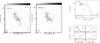 |
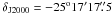
Fig. 1 Shown as contours, emission integrated over the velocity range 0.45 to 59.8 km s-1 for the NH3(1, 1) transition (left) and NH3(2, 2) transition (central) toward IC 342. The contour levels are −3, 3, 6, 9 and 12 times 0.7 mJy km s-1 beam-1 for the (1, 1) map and −3, 3, 6, 9 and 12 times 0.5 mJy km s-1 beam-1 for the (2, 2) map. Overlaid in gray scale for each panel are the radio continuum maps at the respective frequencies (~23.7 GHz) with the upper bars providing the flux density scale in mJy beam-1. An asterisk indicates the location of the (western) water vapor maser detected by Tarchi et al. (2002), while the boxes indicate the areas that were taken for integrating the emission from each ammonia cloud identified from these data. The spectra to the right show the integrated NH3 emission (upper panel) and the spectra toward the four regions depicted in the contour maps (lower panel). |
2. Observations and data reduction
The (J,K) = (1, 1) and (2, 2) inversion transitions of NH3, (rest frequencies: 23.6944955 GHz and 23.7226333 GHz, Lovas 2004), were observed toward IC 342 and Maffei 2 on 22–27 October 2001 using the D configuration of the Very Large Array (VLA) of the NRAO1. The beam sizes are  at a PA −85° for IC 342 and
  at a PA −89° for Maffei 2. We used a bandpass of 25 MHz centered at heliocentric velocities of + 40 km s-1 for IC 342. The heliocentric velocity of Maffei 2 is −40 kms-1, but due to limitations in the LO tuning at the VLA for bandpasses of 25 MHz or more, we set the central velocity to −35 kms-1. The total bandwidth for both sources was divided into 15 spectral channels, each 1.5625 MHz wide (~19.7 km s-1 at the observing frequencies), plus a continuum channel containing the central 75% of the total band. For the amplitude calibration, we used 0137 + 331, with an adopted flux density of 1.05 Jy. The phase calibrators were 0304 + 683 with a flux density of 0.43 Jy, and 0244 + 624 with a flux density of 1.6 Jy at 1.3 cm.
The NH3(3, 3) transition (rest frequency: 23.8701292 GHz, Lovas 2004) was observed toward NGC 253 on 29–30 September 2001 using the VLA DnC configuration. This configuration was required because of the low elevation of this source. The resulting beam size was  at a PA 58°. The observations used a bandwidth of 50 MHz centered at a heliocentric velocity of 9 km s-1 and 16 spectral channels, each of them covering ~40 km s-1. Since the systemic velocity of NGC 253 is at ~ 230 km s-1, the transition is at the edge of the observed band. From a comparison with CO spectra (e.g. Mauersberger et al. 2003) we estimate, however, that ≲ 5% of the flux is outside the observed spectral bandpass. Absolute flux density calibration was obtained by observing 0137+331 (1.05 Jy). Phase and bandpass calibration were performed on 0120−270.
The data were edited and calibrated following the standard VLA procedures and using the Astronomical Image Processing System (AIPS) developed by the NRAO. Observations from different days were combined in the UV plane. We synthesized, cleaned, and naturally weighted maps of the observed regions. For each source, a continuum map was produced by averaging line-free channels.
In order to convert flux density per beam, S, to synthesized beam brightness temperature, Tb, we have used the relation  (1)(see Eq. (8.20) in Rohlfs & Wilson 1996), where θa and θb indicate the full width at half power (FWHP) linewidths of the major and minor axes of the elliptical synthesized beam in arcseconds.
3. Results
3.1. Continuum emission
Figure A.1 shows the λ ~ 1.3 cm continuum of IC 342, Maffei 2, and NGC 253. We estimate that the calibration accuracy of the continuum is ~10%. The 23.7 GHz continuum emission of IC 342 peaks toward  ,
,  with a total flux density of 33 mJy and a maximum of 7.1 mJy/beam. The emission is resolved with an apparent FWHP extent of
  (major × minor axis), which corresponds to a deconvolved source size of
  at a PA of + 78o. This extent is compatible with the observations by Turner & Ho (1983), who separated the thermal from the non-thermal emission. The thermal 6 cm continuum emission determined by these authors is ~40 mJy for IC 342. Considering this flux density and a spectral index α of −0.1 (Sν ∝ να), the expected thermal emission is ~36 mJy at 23.7 GHz, which is consistent with our measured value of 33 mJy.
The 23.7 GHz continuum emission from Maffei 2 is centered at  ,
,  with a total flux density of 40 mJy and a maximum of 8.2 mJy/beam. The emission is resolved with an apparent FWHP extent of
  (major × minor axis), which corresponds to a deconvolved source size of
  at a PA of ~ 0o. This extent is compatible with the higher resolution VLA 2 cm data by Turner & Ho (1994), who found that the extended continuum emission is dominated by non-thermal radiation. They assumed an α of −0.8 for the extended continuum in Maffei 2. The non-thermal component is, however, spatially related to compact thermal sources. Taking the above mentioned spectral index, the expected flux density is 31.8 mJy at 23.7 GHz, and is smaller than our value of 40 mJy. This suggests that a significant fraction of the 23.7 GHz continuum is due to thermal free-free emission.
Toward NGC 253 we have detected 23.7 GHz continuum emission centered at 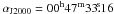 ,
,  with a total flux density of 468 mJy and a maximum of 179 mJy/beam. This flux density is compatible, within the estimated errors, with the data obtained by Geldzahler & Witzel (1981) and Ott et al. (2005). The emission is resolved with an apparent FWHP extent of
  (major × minor axis), which corresponds to a deconvolved source size of
  at a PA of 45o. The spatial extent of this emission is compatible with the higher resolution images obtained by Ulvestad & Antonucci (1997).
3.2. The NH3 emission
Our maps of the NH3 emission toward IC 342, Maffei 2, and NGC 253 confirm that the single dish ammonia spectra previously detected toward these galaxies (Mauersberger et al. 2003) are composed of the contributions of different giant molecular clouds (GMCs). In the analysis of the data, for each identified giant cloud, Gaussians were fitted to the ammonia spectra. Table 1 contains the fit parameters for each GMC for IC 342, Maffei 2, and NGC 253, respectively. The average linewidths for IC 342 are ~40 km s-1 while for Maffei 2 and NGC 253 they are larger by a factor up to four (see Sect. 3.2.3). This, and the low velocity resolution of ~20 km s-1 for IC 342 and Maffei 2 and ~40 km s-1 for NGC 253 does not allow for a deconvolution of the line profiles into velocity sub-structures inside the GMCs or to deconvolve the satellite lines as it has been done for Galactic center clouds (McGary & Ho 2002).
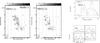 |
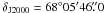
Fig. 2 Images of the velocity-integrated NH3(1, 1) and NH3(2, 2) lines from Maffei 2. The emission was integrated from −135 km s-1 to 62 km s-1. The gray scale images are the continuum maps at the respective frequencies (~23.7 GHz) with the upper bars providing the flux density scale in mJy beam-1. The contour levels are −3, 3, 4, 5, and 6 times 1.3 mJy km s-1 beam-1 for the (1, 1) map and −3, 3, 4, 5, and 6 times 1.8 mJy km s-1 beam-1 for the (2, 2) map. The spectra to the right show the integrated NH3 emission (upper panel) and the spectra toward the four regions depicted in the contour maps (lower panel). |
Gaussian fit parameters, NH3 column densities, and rotational temperatures.
3.2.1. IC 342
Improvements in the performance of the VLA interferometer have resulted in a highly increased dynamic range for our images of the ammonia emission from IC 342 as compared to Ho et al. (1990a). Our channel maps of the ammonia (1, 1) and (2, 2) emission (Fig. A.2) reveal clear substructure not apparent in previous measurements. The ammonia emission is present between 0.4kms-1 and 80 kms-1.
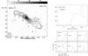 |
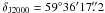
Fig. 3 Left frame: contours show the velocity-integrated NH3(3, 3) transition emission from NGC 253 integrated from 144 km s-1 to 341 km s-1. Overlain is the gray-scale image of the continuum at 23.7 GHz with the upper bar providing the flux density scale in mJy beam-1. The contour levels are −3, 3, 6, 12, 18, 24 times 1.2 mJy km s-1 beam-1. Right upper frame: integrated NH3 (3, 3) spectrum. Right lower frame: ammonia (3, 3) transition spectra integrated over the six clouds of NGC 253 identified by the boxes in the velocity integrated NH3 (3, 3) emission (left panel). |
Figure 1 shows the velocity integrated emission for both transitions. The ammonia emission is concentrated in four main giant clouds. The peak position of each cloud is given in Table 1, while the corresponding spectrum is shown in Fig. 1. Each spectrum was fitted with a single Gaussian in order to obtain the central velocity and the apparent linewidth.
In the regions selected around some of the GMCs (see Fig. 2), the overall velocity integrated fluxes of the (1, 1) and (2, 2) transitions are 0.54 and 0.30 Jy km s-1. This is significantly smaller than the total flux in these lines contained in our maps (1.43 Jy km s-1 for the (1, 1) line and 0.89 Jy km s-1 for the (2, 2) line) and indicates that the regions selected represent only about 35% of the total NH3 emission. Ammonia is therefore not restricted to the main identifiable giant molecular clouds but is also detected from the intercloud gas. Within the calibration uncertainties and accounting for potential differences due to different beam sizes, the measured total flux is similar to the single dish fluxes from Mauersberger et al. (2003) which are 1.1 Jy km s-1 for the (1, 1) line and 1.24 Jy km s-1 for the (2, 2) line. Our interferometric data are therefore not missing significant amounts of single dish flux from the ammonia emission.
3.2.2. Maffei 2
The ammonia (1, 1) and (2, 2) spectral channel measurements of Maffei 2 are shown in Fig. A.3, revealing velocity structure which forms four main giant clouds along a ridge extending from the north-east to the south-west (Fig. 2). There is emission toward all 4 peaks. In addition, in peak B, which is close to the continuum emission peak, the NH3 (2, 2) is seen in absorption against the 1.3 cm continuum in the velocity range between −20 and 100 km s-1. Maffei 2 is located close to the Galactic plane and the line of sight material causes a visual extinction of 5.6 mag (Fingerhut et al. 2007). The NH3 absorption we observe is most likely from gas within Maffei 2 and not from intervening gas in our own Milky Way since a) the observed lines are much wider than a few km s-1 and b) the velocities expected from gas in this quadrant of the Milky Way would be at negative velocities. In Table 1 we give the results of Gaussian fits toward the peaks A–D. The fluxes of the (1, 1) and (2, 2) emission lines contained in the regions A–D are 1.3 and 0.8 Jy km s-1, while the total line flux from these transitions contained in our map is 1.8 and 0.8 Jy km s-1. For the (1, 1) line this indicates that the emission from regions A–D represents 70% of the total flux in the mapped area. Such a percentage may also be representative for the NH3 (2, 2) emission regions, but a direct comparison is not straight forward due to the mixture of emission and absorption features in this line, which are difficult to disentangle. The single dish fluxes from the 40′′ Effelsberg beam are 1.2 and 1.1 Jy km s-1 (Henkel et al. 2000). For the (1, 1) line this is smaller than the total flux in our map, which is expected since the NH3 emitting region in Maffei 2 is not small compared to the Effelsberg beam. In particular, peak D is right at the half power level of the Effelsberg beam.
3.2.3. NGC 253
The left frame of Fig. 3 shows the velocity-integrated emission of the NH3(3, 3) transition. With an overall extent of 40′′ × 5′′ along a PA of ~45°, the NH3 emission is much more extended than the 1.3 cm continuum, which is located near the “center of gravity” of the NH3 emission. The upper right of Fig. 3 shows the integrated spectrum of the NH3(3, 3) emission. The line shape and the flux of 8.6 Jy km s-1 is only slightly smaller than the total flux detected in our maps (11.8 Jy km s-1), which is similar to the single dish spectrum observed by Mauersberger et al. (2003) with a 40′′ beam, which contains a flux of 10.9 Jy km s-1. The flux measured by Ott et al. (2005) with the ATCA interferometer (synthesized beam sizes 19′′ × 5′′ and 30′′ × 5′′) is 8.1 Jy km s-1. Takano et al. (2005a) report a significantly higher value that is 30% higher than ours, namely 15.3 Jy km s-1. This may be to a very small part due to our incomplete spectral coverage of the NH3 (3, 3) line, but mainly reflects the calibration uncertainties at such a low elevation. We will assume in the following that, as for Maffei 2, most of the flux density has been recovered by our measurements.
The NH3 emission arises from six giant clouds, that we label from A to F with increasing right ascension. The lower-right frame of Fig. 3 shows the NH3(3, 3) spectra observed toward each of the six giant clouds (indicated by boxes in the contour map). Each spectrum was fitted with a single Gaussian (see Table 1). Typical linewidths of the individual clouds are of order 70–160 km s-1. This is larger than the velocity separation of the hyperfine (HF) components of the NH3(3, 3) transition. Under conditions of local thermodynamic equilibrium (LTE) and optically thin line emission, the outer hyperfine components have an intensity 2.6% of that of the main component. Therefore, the fitted linewidths should well correspond to the intrinsic linewidths of the clouds. Channel maps of the ammonia (3, 3) emission are shown in Fig. A.4. The ammonia emission is present between 144 km s-1 and 341 km s-1. The latter is the upper limit to the velocity extent of the emission dictated by observational bandwidth limitations (see Sect. 2).
4. NH3 column density and rotational temperature
The total column density of the two states of an ammonia (J,K) inversion doublet is given by ![\begin{equation} N(J,K)=1.65\,10^{14}{\rm cm^{-2}}\nu^{-1}\left[J(J+1)/K^2\right] \Delta v T_{\rm ex}\tau_{\rm tot}, \label{eq:njk} \end{equation}](/articles/aa/full_html/2011/10/aa17533-11/aa17533-11-eq69.png) (2)where ν is the inversion frequency in GHz, Δv is the FWHP linewidth in km s-1, Tex is the excitation temperature in K, and τtot is the sum of the peak optical depths of the five groups of hyperfine (hf) components comprising each inversion transition. For the (J,K) = (1, 1) transition, τtot = 2.000τm (m: main group of hf components); and for the (2, 2) and (3, 3) transitions τtot = 1.256τm, and 1.119τm, respectively. For higher-lying inversion transitions τtot ≃ τm. Assuming that the background continuum can be neglected, the brightness temperature of the main group of hyperfine components Tb of an ammonia transition relates to its excitation temperature as Tb = Tex(1−exp(−τm)), i.e. in the optically thin limit Tb ~ Texτm. Using the transition parameter that can be directly observed, namely the main-beam brightness temperature Tmb, instead of Tb results in beam averaged (instead of source averaged) column densities.
(2)where ν is the inversion frequency in GHz, Δv is the FWHP linewidth in km s-1, Tex is the excitation temperature in K, and τtot is the sum of the peak optical depths of the five groups of hyperfine (hf) components comprising each inversion transition. For the (J,K) = (1, 1) transition, τtot = 2.000τm (m: main group of hf components); and for the (2, 2) and (3, 3) transitions τtot = 1.256τm, and 1.119τm, respectively. For higher-lying inversion transitions τtot ≃ τm. Assuming that the background continuum can be neglected, the brightness temperature of the main group of hyperfine components Tb of an ammonia transition relates to its excitation temperature as Tb = Tex(1−exp(−τm)), i.e. in the optically thin limit Tb ~ Texτm. Using the transition parameter that can be directly observed, namely the main-beam brightness temperature Tmb, instead of Tb results in beam averaged (instead of source averaged) column densities.
The transition optical depths are unknown and cannot be easily determined since Doppler broadening masks individual hyperfine satellite emission. Takano et al. (2005b) claim low optical depths from line-to-continuum ratios of absorption lines toward Arp 220. The latter is, however, also affected by the unknown source covering factor of the molecular gas. From observations of ammonia emission toward molecular clouds toward the Galactic center region, where linewidths are of order 10 km s-1, Hüttemeister et al. (1993) derive optical depths of about two for the main group of hyperfine satellites of the (1, 1) and (2, 2) transitions. They also find higher optical depths toward the stronger peaks of molecular emission. The Galactic Center data presented by Hüttemeister et al. (1993) were obtained with a linear resolution of 1.7 to 3.2 pc, while the VLA beam size toward the galaxies observed corresponds to about 50 pc (see Sect. 1). It is plausible that the source-averaged opacities of the observed NH3 transitions toward our galaxy sample are smaller than the value of ~ 2 determined toward Galactic center clouds, which would suggest that Texτtot ~ Tmb.
The synthesized beam averaged Tmb values are associated with the spectral flux density, Sν, by the relation in Eq. (1). With these assumptions, beam averaged column densities can be derived using  (3)where κ = 6.04, 2.81, 2.21, and 1.47 for the (J,K) = (1, 1), (2, 2), (3, 3) and (6, 6) transitions discussed in this paper, respectively.
The rotational temperature between any (J,J) and (J′,J′) levels can then be determined using ![\begin{equation} T_{\rm rot} = {\Delta E \, ({\rm K})/ {\ln\left[{(2J+1)g_{\rm op}\over (2J'+1)g'_{\rm op}}{{N(J',J')}\over{N(J,J)}}\right]}}\cdot \label{eq:trot} \end{equation}](/articles/aa/full_html/2011/10/aa17533-11/aa17533-11-eq89.png) (4)Here gop is 2 for ortho ammonia (K = 3,6), and 1 for para ammonia (K = 1,2).
(4)Here gop is 2 for ortho ammonia (K = 3,6), and 1 for para ammonia (K = 1,2).
5. Discussion
5.1. IC 342
5.1.1. Distribution and excitation of the molecular gas
Distance estimates toward the nearly face-on and highly obscured spiral galaxy IC 342 range from 1.8 Mpc (McCall 1989) to 8 Mpc (Sandage & Tammann 1974). As a consequence of this distance ambiguity the size and luminosity of this galaxy have been classified as similar to or much in excess of the Galactic values. Recently Tikhonov & Galazutdinova (2010) derived a distance of 3.9 ± 0.1 Mpc using stellar photometry. To facilitate a comparison with previous studies, here we adopt the distance proposed by Saha et al. (2002), 3.3 Mpc. The giant molecular clouds in the central bar of IC 342 (e.g. Sakamoto et al. 1999) have a linear size which is similar to that of the Sgr A and Sgr B2 molecular clouds in the center of our Galaxy. The inner 400 pc of IC 342 have the same far infrared luminosity as the inner 400 pc of our Galaxy and the 2 μm luminosities indicate that the central regions contain similar masses of stars (e.g. Downes et al. 1992). Fortunately, IC 342 is viewed face-on, and its nuclear region is therefore much less obscured than that of the Milky Way, although IC 342 is located behind the Galactic plane (bII ~ 10°).
5.1.2. Comparison of NH3 with other tracers of dense gas in IC 342
According to Downes et al. (1992) and Sakamoto et al. (1999), the highest concentrations of CO and HCN are present in a region of diameter ~40′′ near the nucleus of IC 342. Downes et al. (1992) discussed the presence of at least five molecular complexes, the most interesting of which is “Cloud B” (following the notation of Downes et al.). Only this region is associated with powerful H ii regions, while the other complexes appear to be too hot and too turbulent to form stars with similar efficiency. The nucleus and Cloud B are only ~3′′ apart. The ammonia emission is in the form of four unresolved or poorly resolved maxima along an elongated curved structure of 40′′ (350 pc) length. Four of these maxima can be identified with the HCN maxima A, C, D, and E observed by Downes et al. (1992). The ammonia ridge continues southward of HCN peak E without resolving single GMCs. No NH3 emission can be seen toward “Cloud B”.
When we compare our NH3 (1, 1) and (2, 2) emission with the various interferometric molecular emission maps by Meier & Turner (2001; 2005) and Usero et al. (2006), we find the best correspondence (including the extension south of cloud E) with the distributions of C18O (1−0), CH3OH (methanol) (2k−1k) and N2H+ emission. We also find excellent correspondence with images of H13CO+ (1−0) and SiO (2−1), although in these Plateau de Bure maps the extensions south of Cloud E are not visible as they are outside the primary beam. There is also correspondence between HCN peaks A, C, D, and E and HNCO (404−303), although the extension south of Cloud E is not seen in HNCO. With HNC (1−0), as with HCN (1−0) (Downes et al. 1992), there is good coincidence of peaks A, C, D, and E; however, Cloud B is seen in HNC and HCN but (as already mentioned) not in NH3. The poorest coincidence with our NH3 images is with the distributions of CCH 1−0;3/2−1/2 and C34S 2−1, both of which peak between Cloud A and the continuum peak.
Of the more complex molecules that coincide the best, namely NH3, CH3OH and HNCO, all have in common that they are thought to be liberated from grains by shocks. In order to be released from grain mantles without being destroyed, slow (vshock = 10−15 km s-1) shocks are required (see the discussion in Martín et al. 2006a). Ammonia, methanol and HNCO are easily destroyed by dissociating radiation (Hartquist et al. 1995; Le Teuff et al. 2000). SiO, on the other hand would need fast shocks (vshock ≳ 15−29 km s-1) to be released from grain cores (see the discussion in Usero et al. 2006). Alternatively it has been proposed that SiO can be generated in a high temperature environment in the gas phase (Ziurys et al. 1989). The good coincidence of SiO with the slow shock tracers methanol, ammonia and HNCO would support this latter interpretation. For all the mentioned tracer molecules, our peaks A, C, D and E can clearly be identified, and they all seem to avoid the continuum peak indicating the absence (or effective shielding) of dissociating radiation.
In contrast, C34S, CCH (and also to a certain degree HCN and HNC) are strongly enhanced toward peak B. In the case of CS, this can be explained by a chemical enhancement of the CS abundance of up to > 10-6 due to the presence of a small amount of ionized sulfur (Sternberg & Dalgarno 1995). Also the CCH abundance is predicted to be enhanced in photodissociation regions (see the discussion in Meier & Turner 2005), which would explain its existence toward the only peak associated with H ii regions.
5.1.3. Kinetic temperature in the IC 342 clouds
In Table 1 we list the derived rotational temperatures between the (1, 1) and (2, 2) rotational levels for the four peaks detected in these transitions; values range between 25 K (Clouds D and E) and 36 K (Cloud A). Since the rotational temperatures between the (1, 1) and (2, 2) levels represent only a lower limit to the kinetic temperatures it is interesting to compare these with those derived using higher excitation transitions.
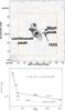 |
Fig. 4 Upper frame: contours showing our IC 342 NH3 (J,K) = (2, 2) image smoothed to the same resolution as the Montero-Castaño et al. (2006) NH3(6, 6) emission image. The gray scale shows the 1.3 mm continuum, and the asterisks denote the three (6, 6) ammonia peaks. The H2O maser detected by Tarchi et al. (2002) is indicated as a cross, while the box indicates the area depicted in Fig. 1. Lower frame: Boltzmann plot for IC 342 peak C and the “continuum” peak using the measured (1, 1), (2, 2) and (6, 6) transitions of NH3. |
The VLA map of the (J,K) = (6, 6) (Eu = 411 K) transition toward IC 342 by Montero-Castaño et al. (2006) allows for a direct comparison with our images of the lower excitation NH3, and thus to study the excitation conditions in the various giant molecular clouds of IC 342. Comparing the maximum of the spectral flux density, S, in their (6, 6) VLA map with Effelsberg data by Mauersberger et al. (2003), Montero-Castaño et al. (2006) conclude that no flux is missing in their NH3 (6, 6) image, i.e. the three peaks represent indeed 100% of the (6, 6) emission. The situation is different if one compares the flux density integrated over the line profiles (i.e. ∫S dv). The total flux in the VLA NH3 (6, 6) image is 242 mJy km s-1, while the Effelsberg spectrum presented by Mauersberger et al. (2003) contains a flux of 330 mJy km s-1, i.e. 27% of the NH3 (6, 6) line flux is missing in the VLA (6, 6) map, most of which is probably in the line wings.
In Fig. 4 we show a version of our NH3 (2, 2) map smoothed to the same angular resolution as the (6, 6) ammonia map of Montero-Castaño (2006). In the NH3 (6, 6) map, which has a resolution of  , three peaks can be identified: the main NH3 (6, 6) peak can be identified with our peak C within an accuracy of 1′′. The second NH3 (6, 6) peak appears to be north of our peaks A and E by 3′′, south of the HCN peak B, and coincides with the 1.3 cm continuum. It is remarkable that this second peak does not coincide well with most other molecular line distributions presented in Meier & Turner (2005), except the HNC (1−0) and the HC3N (10−9) transitions. The third peak, the “Western Peak” observed in NH3 is the most mysterious since it does not coincide with any published molecular distribution, including our NH3 (1, 1) and (2, 2) images, nor with any prominent continuum features. A notable exception is a 1.3 cm water maser discovered by Tarchi et al. (2002; see Sect. 5.1.5), whose positional uncertainty is 5′′. The NH3 (2, 2) peak D, on the other hand, has no counterpart in NH3 (6, 6).
In Fig. 4b we show Boltzmann plots toward the other NH3 (6, 6) peaks. For this comparison the (1, 1) and (2, 2) images were smoothed to the same resolution as the (6, 6) image. This has the consequence that there is also some weak (1, 1) and (2, 2) emission from the continuum peak. We can observe the same behavior as was noted in the various transitions measured with a single dish toward IC 342 by Mauersberger et al (2003). While the rotational temperatures between the (1, 1) and (2, 2) transitions are between 23 K (continuum peak) and 27 K (peak C), the (6, 6)/(2, 2) rotational temperatures are 680 K toward peak C and 920 K toward the continuum peak. These values are higher than the single dish rotational temperature of 440 K fitted by Mauersberger (2003) to the NH3 (5, 5), (6, 6) and (9, 9) data. In a warm environment, radiative transfer simulations predict higher Trot values for the higher-excitation metastable energy levels, gradually approaching TK, even if the gas is characterized by a single kinetic temperature (e.g. Walmsley & Ungerechts 1983; Danby et al. 1988; Flower et al. 1995). Alternatively, there may be several gas components with different temperatures within our beam.
It was noted in Sect. 3.2.1 that within the selected regions our NH3 (1, 1) and (2, 2) transitions recover less than 50% and 75% of the (1, 1) and (2, 2) single dish fluxes, respectively. This will not significantly alter the resulting rotational and/or kinetic temperatures derived from these measurements. The different molecular complexes we have discovered are not much larger than the synthesized beam width of the VLA. There may, though, be an extended emission component within which the measured components are embedded. Furthermore, since the percentage of missing flux is larger for the (2, 2) than for the (1, 1) transition, the rotational temperatures given in Table 1 are lower limits.
5.1.4. The nature of the “peak C” and the “continuum peak”
The NH3 emitting gas in the central region of IC 342 should originate from highly shielded regions since NH3 has a low dissociation energy and can be easily destroyed by a strong energetic radiation field (Saha et al. 1983). The temperatures observed are comparable to the kinetic temperatures of ≳ 600 K found in absorption toward the H ii regions in Sgr B2 (Hüttemeister et al. 1995; Wilson et al. 2006). The hot gas in Sgr B2 is of comparatively low density (<103 cm-3). Hüttemeister et al. (1995) conclude that the gas toward Sgr B2 is probably heated by C-type shocks arguing that this kind of shock is able to liberate large quantities of NH3 from dust mantles and heat them to high temperatures without destroying them. Like in the case of Sgr B2 the CH3OH and SiO observed in IC 342 might be associated with the hot gas component, at least for peak C and the continuum peak.
5.1.5. The nature of the “western peak”
Toward the western peak, no definite (6, 6)/(2, 2) temperature can be derived due to our non detections of the lower excitation transitions of NH3. A similar case where there is a strong presence of NH3 (6, 6) emission with a corresponding lack of emission in the lower excitation transitions of NH3 has also been observed toward our Galactic center (Herrnstein & Ho 2002), although on a much smaller linear scale. This lack of NH3 (1, 1) or (2, 2) emission toward an NH3 (6, 6) emission peak has been explained by a geometric configuration whereby the lower-excitation transitions experience foreground absorption by cool material along the line of sight. However, although this scenario might explain the absence of lower excitation NH3 transitions, it would be difficult to explain why one does not see any other molecular emission toward this position. Alternative mechanisms that can explain the presence of (6, 6) emission but not lower lying transitions include:
-
An overabundance of ortho ammonia (i.e. with K = 0,3,6,...) by a factor of > 2 due to its formation in a very cold (i.e. ≪ 23 K) environment. Unfortunately, this configuration has never been observed in any source in the Galaxy. The hypothesis could be tested by observing the NH3(3, 3) transitions toward the NH3 (6, 6) peak.
-
A more viable hypothesis is that we are observing maser emission in the (6, 6) transition but not in the (1, 1) and (2, 2) transitions. Such a maser as observed toward the Galactic star formation region NGC 6334 I (Beuther et al. 2007) could be detectable even if the column density is comparatively low as the detection of 15NH3 (J,K) = (3, 3) maser emission toward a Galactic hot core suggests (Mauersberger et al. 1986). Ammonia maser activity has also been proposed toward NGC 253: Ott et al. (2005) reported NH3 (3, 3) in emission toward a position where other, higher and lower lying transitions were seen in absorption. In order to prove or discard the hypothesis of NH3 (6, 6) maser activity toward the western peak, one has to perform higher resolution mapping and/or to study other high excitation transitions of ammonia.
5.2. Maffei 2
5.2.1. Distribution and excitation of the molecular gas
The barred, highly inclined (i = 67°) spiral galaxy Maffei 2 at a distance of ~3.3 Mpc (see the discussion in Meier et al. 2008) is one of the nearest starburst galaxies, and hence, can be studied with high spatial resolution. A moderately strong nuclear starburst has been observed in the infrared (Rickard & Harvey 1983) and in radio continuum emission (e.g. Turner & Ho 1994). Its nuclear star formation rate is similar to those of M 83 and NGC 253 (Ho et al. 1990b), but its low Galactic latitude (bII ~ −20′) makes optical studies difficult (e.g. Buta & McCall 1983).
Maffei 2 is a galaxy with strong molecular emission from its central region. CO emission reveals a ~220 pc long bar (Meier et al. 2008), which is distinct from the bar seen at large scale in this galaxy. From the location of dense gas and star formation near the intersections of x1−x2 orbits, Meier et al. (2008) concluded that the starburst in Maffei 2 is triggered by dynamics.
5.2.2. Comparison of NH3 emission with other molecules
Four molecular cloud complexes (designated in our Fig. 2 as NH3 A–D) can be seen in NH3 (1, 1), two of which are situated north of the nucleus and the other two toward the south. The NH3 (2, 2) emission is mainly seen toward the south of the nucleus. The large scale distribution of the NH3 (1, 1) emission in Maffei 2 follows that of the isotopic CO and the HCN (J = 1−0) emission (Meier et al. 2008).
If one goes into a detailed comparison of the various measured molecular distributions, one can see important differences between NH3 and the other molecules. In 12CO (1−0), and also in 13CO (1−0), the emission is not only concentrated toward molecular cloud complexes but also a more widespread diffuse component can be seen. This might arise due to a higher opacity and a better signal to noise ratio in these transitions. The rarer isotopic substitution C18O in its J = 1−0 and 2−1 transitions indicates, on the other hand, a similar contrast as NH3. The 2−1 transitions are reliable tracers of the H2 column density for a large range of H2 densities (Wilson & Mauersberger 1990). In 13CO 2−1, we can well distinguish the four NH3 clouds. Unlike NH3, CO also shows strong emission toward the continuum peak. The detailed distribution of C18O 2−1 differs from the distribution of the NH3 and the 13CO emission. This could be explained in terms of large variations of isotopic abundances of 18O or 13C, contamination by the continuum, or just insufficient signal-to-noise (D. Meyer, priv. comm.). To conclude, the similar distributions of large scale NH3 emission with other tracers of H2 suggests that we are indeed observing a representative fraction of the dense gas in NH3 and that the observed NH3 distribution is not just due to excitation effects or due to varying chemical abundances.
5.2.3. Kinetic temperatures
In Table 1 we show rotational temperatures between the (1, 1) and (2, 2) levels for the four peaks detected in these transitions. Derived rotational temperatures range from 24 K (Clouds C) to 48 K (Cloud B). Since the Trot between the (1, 1) and (2, 2) levels represents only a lower limit to TK, it is interesting to compare these measurements to rotational temperatures derived from higher-excitation NH3 transitions. Unfortunately such higher transitions are only available from single dish measurements (e.g. Henkel et al. 2000; Mauersberger et al. 2003; Takano et al. 2005a). Radial velocity information, can, however, be used for a comparison. From the (1, 1) to (4, 4) transitions, Henkel et al. (2000) suggested that the −80 kms-1 component (Clouds A and B) should be warmer than the component at + 6 kms-1 (Clouds C and D). This is also what is indicated from our high resolution data. On the other hand the inclusion of (6, 6) data by Mauersberger et al. (2003) shows no difference in excitation for the very hot gas. This indicates that although there is very warm gas (130 K) at −80 and at + 6 kms-1, the gas toward the velocity component at + 6 kms-1, i.e. clouds C and D has, on average, lower than average excitation, which could be due to an additional cooler component.
5.3. NGC 253
5.3.1. The distribution of NH3 and other molecules
The Sculptor galaxy NGC 253 is a highly inclined (i ~ 78°) nearby (D ~ 3.5 Mpc, Recola et al. 2005) barred Sc spiral. It is one of the brightest sources of far infrared emission beyond the Magellanic Clouds and has been studied in detail at many wavelengths. NGC 253 hosts a nuclear starburst. Radio continuum measurements indicate that NGC 253 contains a large number of potential centrally located supernova remnants and H ii regions (Ulvestad & Antonucci 1997; Brunthaler et al. 2009).
A nuclear bar has been imaged in the CO, HCN and HCO+ emission lines (Sakamoto et al. 2006; Knudsen et al. 2007), and many other molecules have been detected in NGC 253 (see e.g. the 2 mm line survey of Martín et al. 2006b). Among these, five turned out to be particularly important to reveal the peculiar physical conditions of the starburst region in this galaxy: SO, SiO, HNCO, CH3OH, and CH3CN (Henkel et al. 1987, 1991a; Nguyen-Q-Rieu et al. 1991; Hüttemeister et al. 1997). The abundances of these five molecules have been found to be particularly high in NGC 253. This indicates that in contrast to a “late starburst” such as M 82, where the chemistry is affected by photodissociation, the chemistry in NGC 253 is dominated by slow shocks which are able to release molecules from grains without destroying them (see also García-Burillo et al. 2001; Usero et al. 2004, 2006). Ammonia belongs to the same class of molecules, thought to be enriched in C-shock environments and which is easily destroyed by dissociating radiation due to its low dissociation energy (Suto & Lee 1983).
Takano et al. (2005a) presented VLA maps of the (1, 1), (2, 2), and (3, 3) transitions of NH3. The data presented in this paper only include the ammonia (3, 3) transition but with a higher spatial resolution ( instead of
  ). The agreement between the two (3, 3) maps is good. Comparing this map with a super-resolved NH3 map (resolution: 5′′ × 5′′) by Ott et al. (2005) we find excellent agreement with the locations of clouds A, B and C, while clouds D, E and F are shifted between 2 to 5′′ with respect their peak positions. This discrepancy can probably be explained by the deconvolution process used by Ott et al. (2005). There is also good agreement between the features seen in our map and the
  resolution maps of HCN and HCO+ presented by Knudsen et al. (2007).
The individual GMCs in NGC 253 are more pronounced in NH3 than in HCN or HCO+. This may be due to the fact that the latter transitions being optically thick, and therefore the contrast between the clouds and the intercloud gas does not reflect the contrast in column density of HCN or HCO+. Another notable difference is that our Cloud B is about 3′′ north of the nearest HCN and HCO+ feature. This HCN and HCO+ feature, where no NH3 is measured, corresponds in location and velocity to one of the two “molecular superbubbles” identified by Sakamoto et al. (2006), and is within the positional uncertainties identical to the superbubble already seen in the NH3 data of Ott et al. (2005). Also toward the other superbubble seen in the CO data presented by Sakamoto et al. (2006) and being located in the northeastern edge of the measured NH3 distribution (Fig. 3), weak HCN and HCO+ emission can be seen at the correct velocity, but no NH3. At the opposite edge of the NH3 distribution, our Cloud A is clearly visible in HCN, but not in HCO+.
The agreement of the NH3 distribution with that of 12CO (2−1), 13CO (2−1), 13CO (3−2) and C18O (2−1) measured by Sakamoto et al. (2011) is excellent. Taking into account our sightly coarser resolution we can reproduce all the details in the distribution of those transitions. Since CO isotopes are thought to be among the most reliable tracers of the H2 column density, this supports our notion that NH3 traces the bulk of the gas in the central molecular zone of NGC 253. The reason may be that at the high temperatures in this region the abundance of NH3, which otherwise can vary by several orders of magnitude due to freeze out onto grains, is quite constant, since all NH3 is in the gas phase. The same may be true for the central molecular zone of the Milky Way, which has similarly high temperatures to a degree that even SiO can be observed throughout the region (Riquelme et al. 2010).
To conclude, our NH3 distribution follows closely that of C18O (2–1), which is thought to be an excellent indicator of molecular hydrogen. This suggests that the temperatures derived from NH3 are representative of the bulk of the molecular gas in the central region of NGC 253. HCN and HCO+ also follow the general H2 distribution. However, their emission is, with respect to NH3, enhanced toward regions where fast shocks and/or photodissociating radiation can be expected.
5.3.2. Ammonia maser emission or unusual ortho/para ratios?
Takano et al. (2002) noted that the (3, 3) transition was stronger than expected toward NGC 253, and concluded that an anomalous ammonia ortho/para ratio was the cause. Also Ott et al. (2005) explained the unexpectedly high intensity of the (3, 3) transition toward the NE peak in terms of an ortho/para ratio for ammonia of 2.5–3.5. On the other hand, Ott et al. (2005) also mention that toward the continuum position of NGC 253 they measure the (3, 3) transition in emission, whereas all other transitions are observed in absorption. This would suggest that maser emission in the (3, 3) transition is the cause of the higher than anticipated intensities, which is amplifying the background continuum.
In our measurements of the integrated (3, 3) spectrum (see Fig. 3) the high velocity SW component (V ~ 300 kms-1) is brighter than the lower velocity NE component (V ~ 160 kms-1). This is contrary to the lower resolution data presented by Ott et al. (2005) and Mauersberger et al. (2003) where the 170 km s-1 component is equal in intensity or stronger than the 300 km s-1 component. Note that consistently in all other ammonia transitions observed by Mauersberger et al. (2003) and Ott et al. (2005) the 300 km s-1 component is the strongest. The flux density of the 170 km s-1 component is comparable in our measurements and those presented by Ott et al. The 300 km s-1 component, on the other hand, is 50% stronger in our measurements. From the channel maps in Fig. 3 and also from Takano et al. (2005a), it appears as if this extra flux could come from cloud C (clouds SW1 in the notation of Takano et al. 2005a) which is close to the continuum peak.
How can the different profiles be explained other than by calibration uncertainties and errors? One possibility is time variable emission on a time scale of a few years. If the (3, 3) transition is masing this would imply that the emission comes from a region small in angular extent near the center of NGC 253. Such maser emission would also imply that the intensity is very high within a very narrow transition linewidth.
Inconsistent sensitivity to spatial structure could be an alternative explanation. The situation here is that the higher resolution VLA map results in a higher line flux than that derived from the Australia Telescope Compact Array (ATCA) image presented by Ott et al. (2005). If there is some large scale absorption component on top of the emission from the GMCs, this might be “missed” by the VLA but not by the ATCA and may explain why the 300 km s-1 component is stronger with the VLA than with ATCA. Apparently higher spatial and spectral resolution observations not only of the (3, 3) transition but also of other ortho or para transitions are necessary to settle this issue.
6. Conclusions
Imaging measurements of the NH3 (J,K) = (1, 1) and (2, 2) transitions toward IC 342 and Maffei 2 and of the NH3 (3, 3) transition toward NGC 253 have been presented. Derived lower-limits to the kinetic temperatures determined for the giant molecular clouds in the centers of these galaxies are between 25 and 50 K. In general, there is good agreement between the distributions of NH3 and other H2 tracers, suggesting that NH3 is representative of the distribution of dense gas in these galaxies.
For IC 342, a comparison to high resolution NH3 data indicates a molecular component with kinetic temperatures as high as 700–900 K. Furthermore, the “Western Peak” of IC 342, also known to host an H2O maser, is observed in the NH3 (6, 6) transition but not in lower-excitation NH3 transitions. This is suggestive of maser emission in the (6, 6) transition.
Comparing the (3, 3) line profile from NGC 253 with those obtained from earlier lower resolution studies, the V ~ 300 km s-1 component appears to be enhanced. Explanations could involve a time variable (3, 3) maser or a large scale absorption component not seen by us.
Online material
Appendix A: Additional figures
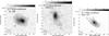 |
Fig. A.1 Continuum maps at 23.7 GHz for IC 342 (left), Maffei 2 (middle), and NGC 253 (right). The contour levels are, −0.3, 0.3, 0.6, 1.2, 2.4, 4.8 mJy beam-1 for IC 342, −0.6, 0.6, 1.2, 2.4, 4.8 mJy beam-1 for Maffei 2, and −2.7, 2.7, 5.4, 10.8, 21.6, 43.2, 86.4 mJy beam-1 for NGC 253. The beams are shown at the bottom left corner of each map. |
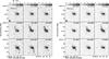 |
Fig. A.2 Channel maps of the NH3(1, 1) and NH3(2, 2) transition emission from IC 342. The contour levels are −0.9, 0.9, 1.8, 2.7, and 3.6 mJy beam-1 and −0.75, 0.75, 1.5, 2.25, and 3 mJy beam-1, respectively. The synthesized beams are shown in the lower left corner of the first panel for each transition. The gray scale images represent the continuum emission at 23.7 GHz. |
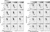 |
Fig. A.3 Channel maps of the NH3(1, 1) and NH3(2, 2) emission from Maffei 2. The contour levels are −0.78, 0.78, 1.56, 2.34, and 3.12 mJy beam-1 and −1.2, 1.2, 2.4, 3.6, and 4.8 mJy beam-1, respectively. The gray scale images show the continuum emission at 23.7 GHz. Beams are shown in the left upper panel for each map set. |
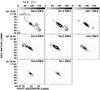 |
Fig. A.4 Channel maps of the NH3(3, 3) transition from NGC 253. The contour levels are −1.8, 1.8, 3.6, 5.4, 7.2, and 9.0 mJy beam-1. The synthesized beam is shown in the left lower corner in the first panel. The gray scale images represent the continuum emission at 23.7 GHz. |
Acknowledgments
We thank the referee, Jean Turner, for excellent suggestions which improved this work. Rainer Mauersberger has been supported by a grant (AYA2005-07516) of the Ministerio de Educación y Ciencias of Spain.
References
- Aladro, R., Martín-Pintado, J., Martín, S., Mauersberger, R., & Bayet, E. 2011, A&A, 525, A89 [NASA ADS] [CrossRef] [EDP Sciences] [Google Scholar]
- Beuther, H., Walsh, A. J., Thorwirth, S., et al. 2007, A&A, 466, 989 [NASA ADS] [CrossRef] [EDP Sciences] [Google Scholar]
- Brinchmann, C. S., White, S. D. M., et al. 2004, MNRAS, 351, 1151 [NASA ADS] [CrossRef] [Google Scholar]
- Brunthaler, A., Castangia, P., Tarchi, A., et al. 2009, A&A, 497, 103 [NASA ADS] [CrossRef] [EDP Sciences] [Google Scholar]
- Buta, R. J., & McCall, M. L. 1983, MNRAS, 205, 131 [NASA ADS] [Google Scholar]
- Costagliola, F., & Aalto, S. 2010, A&A, 515, A71 [NASA ADS] [CrossRef] [EDP Sciences] [Google Scholar]
- Combes, F. 2005, The evolution of starbursts: The 331st Wilhelm and Else Heraeus Seminar, AIP Conf. Proc., 783, 43 [Google Scholar]
- Danby, G., Flower, D. R., Valiron, P., Schilke, P., & Walmsley, C. M. 1988, MNRAS, 235, 229 [NASA ADS] [CrossRef] [Google Scholar]
- Downes, D., Radford, S. J. E., Guilloteau, S., et al. 1992, A&A, 262, 424 [NASA ADS] [Google Scholar]
- Fingerhut, R. L., Lee, H., McCall, M. L., & Richer, M. G. 2007, ApJ, 655, 814 [NASA ADS] [CrossRef] [Google Scholar]
- Flower, D. R., Pineau des Forêts, G., & Walmsley, C. M. 1995, A&A, 294, 815 [NASA ADS] [Google Scholar]
- García-Burillo, S., Martín-Pintado, J., Fuente, A., & Neri, R. 2001, ApJ, 563, L27 [NASA ADS] [CrossRef] [Google Scholar]
- Geldzahler, B. J., & Witzel, A. 1981, AJ, 86, 1306 [NASA ADS] [CrossRef] [Google Scholar]
- Güsten, R. 1989, in The Center of the Galaxy, ed. M. Morris (Dordrecht: Kluwer), 89 [Google Scholar]
- Hartquist, T. W., Menten, K. M., Lepp, S., & Dalgarno, A. 1995, MNRAS, 272, 184 & [NASA ADS] [CrossRef] [Google Scholar]
- Henkel, C., Jacq, T., Mauersberger, R., Menten, K. M., & Steppe, H. 1987, A&A, 188, L1 [NASA ADS] [Google Scholar]
- Henkel, C., Mauersberger, R., Peck, A. B., Falcke, H., & Hagiwara, Y. 2000, A&A, 361, L45 [NASA ADS] [Google Scholar]
- Henkel, C., Jethava, N., Kraus, A., et al. 2005, A&A, 440, 893 [NASA ADS] [CrossRef] [EDP Sciences] [Google Scholar]
- Henkel, C., Braatz, J. A., Menten, K. M., & Ott, J. 2008, A&A, 485, 451 [NASA ADS] [CrossRef] [EDP Sciences] [Google Scholar]
- Herrnstein, R. M., & Ho, P. T. P. 2002, ApJ, 579, L83 [NASA ADS] [CrossRef] [Google Scholar]
- Ho, P. T. P., & Townes, C. H. 1983, ARA&A, 21, 239 [NASA ADS] [CrossRef] [Google Scholar]
- Ho, P. T. P., Beck, S. C., & Turner, J. L. 1990a, ApJ, 349, 57 [NASA ADS] [CrossRef] [Google Scholar]
- Ho, P. T. P., Martin, R. N., Turner, J. L., & Jackson, J. M. 1990b, ApJ, 355, L19 [NASA ADS] [CrossRef] [Google Scholar]
- Hüttemeister, S., Wilson, T. L., Bania, T. M., & Martin-Pintado, J. 1993, A&A, 280, 255 [NASA ADS] [Google Scholar]
- Hüttemeister, S., Wilson, T. L., Mauersberger, R., et al. 1995, A&A, 294, 667 [NASA ADS] [Google Scholar]
- Hüttemeister, S., Mauersberger, R., & Wilson, T. L. 1997, A&A, 326, 59 [NASA ADS] [Google Scholar]
- Knudsen, K. K., Walter, F., Weiss, A., et al. 2007, ApJ, 666, 156 [NASA ADS] [CrossRef] [Google Scholar]
- LeTeuff, Y. H., Millar, T. J., & Markwick, A. J. 2000, A&AS, 146, 157 [NASA ADS] [CrossRef] [EDP Sciences] [MathSciNet] [PubMed] [Google Scholar]
- Lovas, F. J. 2004, J. Phys. Ref. Data, 33, 177 [Google Scholar]
- Martin, R. N., & Ho, P. T. P. 1986, ApJ, 308, L7 [NASA ADS] [CrossRef] [Google Scholar]
- Martín, S., Martín-Pintado, J., & Mauersberger, R. 2006a, A&A, 450, L13 [NASA ADS] [CrossRef] [EDP Sciences] [Google Scholar]
- Martín, S., Mauersberger, R., Martín-Pintado, J., Henkel, C., & García-Burillo, S. 2006b, ApJS, 164, 450 [NASA ADS] [CrossRef] [Google Scholar]
- Mauersberger, R., & Henkel, C. 1989, A&A, 223, 79 [NASA ADS] [Google Scholar]
- Mauersberger, R., & Henkel, C. 1991, A&A, 245, 457 [NASA ADS] [Google Scholar]
- Mauersberger, R., Wilson, T. L., & Henkel, C. 1986, A&A, 160, L13 [NASA ADS] [Google Scholar]
- Mauersberger, R., Henkel, C., & Chin, Y.-N. 1995, A&A, 294, 23 [NASA ADS] [Google Scholar]
- Mauersberger, R., Henkel, C., Weiß, A., Peck, A. B., & Hagiwara, Y. 2003, A&A, 403, 561 [NASA ADS] [CrossRef] [EDP Sciences] [Google Scholar]
- McCall, M. L. 1989, AJ, 97, 1341 [NASA ADS] [CrossRef] [Google Scholar]
- McGary, R. S., & Ho, P. T. P. 2002, ApJ, 577, 757 [NASA ADS] [CrossRef] [Google Scholar]
- Meier, D. S., & Turner, J. L. 2000, ApJ, 531, 200 [NASA ADS] [CrossRef] [Google Scholar]
- Meier, D. S., & Turner, J. L. 2001, ApJ, 551, 687 [NASA ADS] [CrossRef] [Google Scholar]
- Meier, D. S., & Turner, J. L. 2005, ApJ, 618, 259 [NASA ADS] [CrossRef] [Google Scholar]
- Meier, D. S., Turner, J. L., & Hurt, R. L. 2008, ApJ, 675, 281 [NASA ADS] [CrossRef] [Google Scholar]
- Montero-Castaño, M., Herrnstein, R. M., & Ho, P. T. P. 2006, ApJ, 646, 919 [NASA ADS] [CrossRef] [Google Scholar]
- Nguyen-Q-Rieu, Henkel, C., Jackson, J. M., & Mauersberger, R. 1991, A&A, 241, L33 [NASA ADS] [Google Scholar]
- Oka, T., Geballe, T. R., Goto, M., Usuda, T., & McCall, B. J. 2005, ApJ, 632, 882 [NASA ADS] [CrossRef] [Google Scholar]
- Ott, J., Weiß, A., Henkel, C., & Walter, F. 2005, ApJ, 629, 767 [NASA ADS] [CrossRef] [Google Scholar]
- Rekola, R., Richer, M. G., McCall, M. L., et al. 2005, MNRAS, 361, 330 [NASA ADS] [CrossRef] [Google Scholar]
- Rickard, L. J., & Harvey, P. M. 1983, ApJ, 268, L7 [NASA ADS] [CrossRef] [Google Scholar]
- Riquelme, D., Bronfman, L., Mauersberger, R., May, J., & Wilson, T. L. 2010, A&A, 523, A45 [NASA ADS] [CrossRef] [EDP Sciences] [Google Scholar]
- Rohlfs, K., & Wilson, T. L. 1996, Tools of Radioastronomy (Springer Verlag) [Google Scholar]
- Saha, A., Claver, J., & Hoessel, J. G. 2002, AJ, 124, 838 [Google Scholar]
- Sakamoto, K., Okumura, S. K., Ishizuki, S., & Scoville, N. Z. 1999, ApJ, 525, 691 [NASA ADS] [CrossRef] [Google Scholar]
- Sakamoto, K., Ho, P. T. P., Daisuke, I., et al. 2006, ApJ, 636, 685 [NASA ADS] [CrossRef] [Google Scholar]
- Sakamoto, K., Mao, R., Masushita, S., et al. 2011, ApJ, 735, 19 [NASA ADS] [CrossRef] [Google Scholar]
- Sandage, A., & Tammann, G. A. 1974, ApJ, 194, 559 [NASA ADS] [CrossRef] [Google Scholar]
- Sternberg, A., & Dalgarno, A. 1995, ApJS, 99, 565 [NASA ADS] [CrossRef] [Google Scholar]
- Suto, M., & Lee, L. C., 1983, J. Chem. Phys., 78, 4515 [NASA ADS] [CrossRef] [Google Scholar]
- Takano, S., Nakai, N., Kawaguchi, K., & Takano, T. 2000, PASJ, 52, L67 [NASA ADS] [Google Scholar]
- Takano, S., Nakai, N., Kawaguchi, K. 2002, PASJ, 54, 195 [NASA ADS] [CrossRef] [Google Scholar]
- Takano, S., Hofner, P., Winnewisser, G., Nakai, N., & Kawaguchi, K. 2005a, PASJ, 57, 549 [NASA ADS] [Google Scholar]
- Takano, S., Nakanishi, K., Nakai, N., & Takano, T. 2005b, PASJ, 57, L29 [NASA ADS] [Google Scholar]
- Tarchi, A., Henkel, C., Peck, A. B., & Menten, K. M. 2002, A&A, 385, 1049 [NASA ADS] [CrossRef] [EDP Sciences] [Google Scholar]
- Tikhonov, N. A., & Galazutdinova, O. A. 2010, AstL, 36, 167 [Google Scholar]
- Turner, J. L., & Ho, P. T. P. 1983, ApJ, 268, L79 [NASA ADS] [CrossRef] [Google Scholar]
- Turner, J. L., & Ho, P. T. P. 1994, ApJ, 421, 122 [NASA ADS] [CrossRef] [Google Scholar]
- Ulvestad, J. S., & Antonucci, R. R. J. 1997, ApJ, 488, 621 [NASA ADS] [CrossRef] [Google Scholar]
- Usero, A., García-Burillo, S., Fuente, A., Martín-Pintado, J., & Rodríguez-Fernández, N. J. 2004, A&A, 419, 897 [NASA ADS] [CrossRef] [EDP Sciences] [Google Scholar]
- Usero, A., García-Burillo, S., Martín-Pintado, J., Fuente, A., & Neri, R. 2006, A&A, 448, 457 [NASA ADS] [CrossRef] [EDP Sciences] [Google Scholar]
- Walmsley, C. M., & Ungerechts, H. 1983, A&A, 122, 164 [NASA ADS] [Google Scholar]
- Weiß, A., Neininger, N., Henkel, C., Stutzki, J., & Klein, U. 2001, ApJ, 554, L143 [NASA ADS] [CrossRef] [Google Scholar]
- Weiß, A., Downes, D., Neri, R., et al. 2007, A&A, 467, 955 [NASA ADS] [CrossRef] [EDP Sciences] [Google Scholar]
- Wilson, T. L., & Mauersberger, R. 1990, A&A, 239, 305 [NASA ADS] [Google Scholar]
- Wilson, T. L., Henkel, C., & Hüttemeister, S. 2006, A&A, 460, 533 [NASA ADS] [CrossRef] [EDP Sciences] [Google Scholar]
- Ziurys, L. M., Friberg, P., & Irvine, W. M. 1989, ApJ, 343, 201 [NASA ADS] [CrossRef] [PubMed] [Google Scholar]
All Tables
All Figures
|
Fig. 1 Shown as contours, emission integrated over the velocity range 0.45 to 59.8 km s-1 for the NH3(1, 1) transition (left) and NH3(2, 2) transition (central) toward IC 342. The contour levels are −3, 3, 6, 9 and 12 times 0.7 mJy km s-1 beam-1 for the (1, 1) map and −3, 3, 6, 9 and 12 times 0.5 mJy km s-1 beam-1 for the (2, 2) map. Overlaid in gray scale for each panel are the radio continuum maps at the respective frequencies (~23.7 GHz) with the upper bars providing the flux density scale in mJy beam-1. An asterisk indicates the location of the (western) water vapor maser detected by Tarchi et al. (2002), while the boxes indicate the areas that were taken for integrating the emission from each ammonia cloud identified from these data. The spectra to the right show the integrated NH3 emission (upper panel) and the spectra toward the four regions depicted in the contour maps (lower panel). |
| In the text | |
|
Fig. 2 Images of the velocity-integrated NH3(1, 1) and NH3(2, 2) lines from Maffei 2. The emission was integrated from −135 km s-1 to 62 km s-1. The gray scale images are the continuum maps at the respective frequencies (~23.7 GHz) with the upper bars providing the flux density scale in mJy beam-1. The contour levels are −3, 3, 4, 5, and 6 times 1.3 mJy km s-1 beam-1 for the (1, 1) map and −3, 3, 4, 5, and 6 times 1.8 mJy km s-1 beam-1 for the (2, 2) map. The spectra to the right show the integrated NH3 emission (upper panel) and the spectra toward the four regions depicted in the contour maps (lower panel). |
| In the text | |
|
Fig. 3 Left frame: contours show the velocity-integrated NH3(3, 3) transition emission from NGC 253 integrated from 144 km s-1 to 341 km s-1. Overlain is the gray-scale image of the continuum at 23.7 GHz with the upper bar providing the flux density scale in mJy beam-1. The contour levels are −3, 3, 6, 12, 18, 24 times 1.2 mJy km s-1 beam-1. Right upper frame: integrated NH3 (3, 3) spectrum. Right lower frame: ammonia (3, 3) transition spectra integrated over the six clouds of NGC 253 identified by the boxes in the velocity integrated NH3 (3, 3) emission (left panel). |
| In the text | |
|
Fig. 4 Upper frame: contours showing our IC 342 NH3 (J,K) = (2, 2) image smoothed to the same resolution as the Montero-Castaño et al. (2006) NH3(6, 6) emission image. The gray scale shows the 1.3 mm continuum, and the asterisks denote the three (6, 6) ammonia peaks. The H2O maser detected by Tarchi et al. (2002) is indicated as a cross, while the box indicates the area depicted in Fig. 1. Lower frame: Boltzmann plot for IC 342 peak C and the “continuum” peak using the measured (1, 1), (2, 2) and (6, 6) transitions of NH3. |
| In the text | |
|
Fig. A.1 Continuum maps at 23.7 GHz for IC 342 (left), Maffei 2 (middle), and NGC 253 (right). The contour levels are, −0.3, 0.3, 0.6, 1.2, 2.4, 4.8 mJy beam-1 for IC 342, −0.6, 0.6, 1.2, 2.4, 4.8 mJy beam-1 for Maffei 2, and −2.7, 2.7, 5.4, 10.8, 21.6, 43.2, 86.4 mJy beam-1 for NGC 253. The beams are shown at the bottom left corner of each map. |
| In the text | |
|
Fig. A.2 Channel maps of the NH3(1, 1) and NH3(2, 2) transition emission from IC 342. The contour levels are −0.9, 0.9, 1.8, 2.7, and 3.6 mJy beam-1 and −0.75, 0.75, 1.5, 2.25, and 3 mJy beam-1, respectively. The synthesized beams are shown in the lower left corner of the first panel for each transition. The gray scale images represent the continuum emission at 23.7 GHz. |
| In the text | |
|
Fig. A.3 Channel maps of the NH3(1, 1) and NH3(2, 2) emission from Maffei 2. The contour levels are −0.78, 0.78, 1.56, 2.34, and 3.12 mJy beam-1 and −1.2, 1.2, 2.4, 3.6, and 4.8 mJy beam-1, respectively. The gray scale images show the continuum emission at 23.7 GHz. Beams are shown in the left upper panel for each map set. |
| In the text | |
|
Fig. A.4 Channel maps of the NH3(3, 3) transition from NGC 253. The contour levels are −1.8, 1.8, 3.6, 5.4, 7.2, and 9.0 mJy beam-1. The synthesized beam is shown in the left lower corner in the first panel. The gray scale images represent the continuum emission at 23.7 GHz. |
| In the text | |
Current usage metrics show cumulative count of Article Views (full-text article views including HTML views, PDF and ePub downloads, according to the available data) and Abstracts Views on Vision4Press platform.
Data correspond to usage on the plateform after 2015. The current usage metrics is available 48-96 hours after online publication and is updated daily on week days.
Initial download of the metrics may take a while.