| Issue |
A&A
Volume 533, September 2011
|
|
|---|---|---|
| Article Number | A37 | |
| Number of page(s) | 10 | |
| Section | Galactic structure, stellar clusters and populations | |
| DOI | https://doi.org/10.1051/0004-6361/201117275 | |
| Published online | 24 August 2011 | |
HST-ACS photometry of the isolated dwarf galaxy VV124=UGC 4879
Detection of the blue horizontal branch and identification of two young star clusters⋆,⋆⋆
1
INAF - Osservatorio Astronomico di Bologna, via Ranzani 1,
40127
Bologna,
Italy
e-mail: michele.bellazzini@oabo.inaf.it
2
Netherlands Institute for Radio Astronomy (ASTRON), Postbus 2,
7990 AA Dwingeloo, The Netherlands Kapteyn Astronomical Institute, University of
Groningen, Postbus
800, 9700 AV
Groningen, The
Netherlands
Received: 17 May 2011
Accepted: 9 July 2011
We present deep V and I photometry of the isolated dwarf galaxy VV124=UGC 4879, obtained from archival images taken with the Hubble Space Telescope – Advanced Camera for Surveys. In the color-magnitude diagrams of stars at distances greater than 40″ from the center of the galaxy, we clearly identify a well-populated, old horizontal branch (HB) for the first time. We show that the distribution of these stars is more extended than that of red clump stars. This implies that very old and metal-poor populations dominate in the outskirts of VV124. We also identify a massive (M = 1.2 ± 0.2 × 10⁴ M⊙) young (age = 250 ± 50 Myr) star cluster (C1), as well as another of younger age (C2, ≲30 ± 10 Myr) with a mass similar to classical open clusters (M ≤ 3.3 ± 0.5 × 10³ M⊙). Both clusters lie at projected distances less than 100 pc from the center of the galaxy.
Key words: galaxies: dwarf / Local Group / galaxies: structure / galaxies: stellar content / galaxies: individual: UGC 4879 / galaxies: ISM
Based on observations made with the NASA/ESA Hubble Space Telescope, obtained at the Space Telescope Science Institute, which is operated by the Association of Universities for Research in Astronomy, Inc., under NASA contract NAS 5-26555. These observations are associated with program GO-11584 [P.I.: K. Chiboucas].
Photometry catalogue is only available at the CDS via anonymous ftp to cdsarc.u-strasbg.fr (130.79.128.5) or via http://cdsarc.u-strasbg.fr/viz-bin/qcat?J/A+A/533/A37
© ESO, 2011
1. Introduction
The dwarf galaxy VV124=UGC 4879 has been recently recognized to lie at the outer fringes of the Local Group (LG), near the turn-around radius (Kopylov et al. 2008; Tikhonov et al. 2010). It is extremely isolated, being at ≃1.3 Mpc from the nearest giant galaxy (the Milky Way) and at ≃0.7 Mpc from the nearest dwarf (Leo A).
In Bellazzini et al. (2011, Paper I hereafter) we presented new deep wide-field photometry of VV124, which allowed us to confirm and refine the distance estimate by Kopylov et al. (2008), to study in some detail the stellar content of the galaxy and, in particular, its structure out to large radii, revealing the presence of low surface brightness structures in the outskirts. We also presented the first detection of H i in VV124, obtained with the Westerbork Synthesis Radio Telescope (WSRT). 106 M⊙ of H i were found, with a maximum column density of ≳50 × 1019 cm-2. It is worth noting that the distribution of H i is less extended than the stellar body of the galaxy.
Jacobs et al. (2011, J11 hereafter) present Hubble Space Telescope (HST) – Advanced Camera for Surveys (ACS) observations of VV124, resolving the stars very well down to F814W ≃ 27, also in the most central region of the galaxy. In particular, they studied the stellar content in the innermost 40″ (see their Fig. 1), deriving the star formation history (SFH) in that region by means of the synthetic color-magnitude diagram (CMD) technique (see, for example Rizzi et al. 2002; Cignoni & Tosi 2010, and references therein). J11 conclude that most of the SF (≃93 percent of the total, in mass) occurred at the earliest epochs between 14 and 10 Gyr ago. After this, the SF ceased until 1 Gyr ago, when ≃6 percent was formed between 1 and 0.5 Gyr ago and nearly 1 percent in the last 0.5 Gyr. The derived SFH is similar to that observed in other nearby dwarf irregular/transition-type galaxies (see, for example Weisz et al. 2011). The prevalence of old stars seems to increase at greater distances from the center (see also Paper I). From the morphology of the blue-loop region, J11 infer that the metallicity of the youngest stars is [M/H] = −0.7.
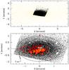 |
Fig. 1 Upper panel: stars detected in the ACS images (dark dots) are superposed to the stars from the LBT sample of Paper I (gray dots) in a projected coordinate system centered on the center of VV124 and rotated to have the X axis coincide with the major axis of the galaxy (see Paper I). Only stars brighter than I = 26.5 from the ACS sample have been plotted, for clarity. Lower panel: zoomed view of the central part of the ACS sample in the same coordinate system. Two concentric ellipses of semi-major axis a = 1.0′ and a = 1.5′, with the same orientation and ellipticity of the galaxy isophotes (see Paper I) are overplotted (in white and in black, respectively). The white circle has a radius Rp = 40″, enclosing the region studied by J11. Blue stars lying on the young main sequence (YMS; −0.4 ≤ V − I ≤ 0.0 and I < 25.5, see Fig. 3) are plotted as red filled circles, the brightest ones (having I ≤ 23.0) are encircled in orange. |
In the present contribution, we use the same observational material of J11 to address three issues raised in Paper I and not considered by J11. These are, in particular:
-
The tentative detection of an extended horizontal branch (HB),including stars in the color range of RR Lyrae variables and blueHB stars, in the CMD of the less-crowded outer regions of thegalaxy (see Fig. 9 of Paper I). WhileJ11 report that a population of HB stars reachingV − I ~ 0.4 is likely present in their CMD, its clean identification and quantification is hampered by the overlap with the young main sequence (MS) in the central region they consider. It would be interesting to search for the HB in the outer portion (Rp > 40″) of the ACS field, where young stars should be quite rare and the old component should be dominant.
-
A possible correlation was noted between the asymmetric distributions of the young stars and of the neutral hydrogen. Since the young population is concentrated in the innermost part of the galaxy, it can be traced in much deeper detail with the ACS data. This, in turn, prompts a more stringent comparison with the H i distribution.
-
We identified a candidate cluster located near the center of the galaxy and within the sheet of young stars (Cluster 1, C1 hereafter). The integrated spectrum of the source, shown in Paper I, shows strong Hβ in absorption, suggesting a young age. With the high spatial resolution ACS image, we can hope to ascertain the real nature of C1 and look for other conspicuous clusters, if any.
There is no reason to repeat the excellent analysis of J11, so we focus strictly on the scientific cases listed above. In the following, we adopt the parameters of VV124 derived in Paper I (see their Table 1), if not stated otherwise. In particular, we adopt D = 1.3 Mpc (in good agreement with J11) and E(B − V) = 0.015 (from Schlegel et al. 1998). At this distance 1″ corresponds to 6.3 pc, 1′ to 378 pc. We also adopt the deprojected coordinate system X,Y of Paper I, centered on the center of VV124 and rotated to let the X axis coincide with the major axis of the galaxy. Finally, we use the elliptical radial distance from the center of the galaxy rϵ. To give an example, stars fulfilling the condition rϵ ≤ 1′ are enclosed within an ellipse whose major axis coincides with the major axis of VV124 and has a = 1′ and ϵ = 0.44 (see Fig. 1, below). The normal (projected) radial distance from the center of the galaxy will be denoted by Rp. All theoretical models used for comparison with observed CMDs are from the (canonical, solar-scaled) BASTI set (Pietrinferni et al. 2004; Percival et al. 2009), in the native ACS- Wide Field Channel (WFC) VEGAMAG system1.
The plan of the paper is as follows. In Sect. 2 we describe the observational material and the data reduction process, and in Sect. 3 we present the clear detection of the extended HB in the external regions of the ACS field and discuss the radial distribution of the various stellar populations of VV124. Section 4 is devoted to a brief discussion of the correlation between the spatial distribution of the H i and of the young stars, and in Sect. 5 we study the candidate luminous star clusters identified here and in Paper I. Finally we briefly summarize and discuss our main results in Sect. 6.
2. Observations and data reduction
The observational material consists of two pairs of F606W and F814W ACS-WFC2 images obtained within the program GO-11584, which we retrieved from the HST archive. The total exposure time of the stacked drizzled images is 1140 s for the F606W and 1150 s for the F814W image. The WFC is a mosaic of two 4096 × 2048 px2 CCDs, with a pixel scale of 0.05 arcsec px-1. The center of VV124 is placed at the center of one of the mosaic chips (chip 1).
Positions and photometry of individual stars were obtained with the ACS module of the point spread function (PSF) – fitting package DOLPHOT v.1.13 (Dolphin 2000), as described, for example, in Galleti et al. (2006). The package identifies the sources on a reference image (in this case the drizzled F814W image, as in Mackey et al. 2006) and performs the photometry on individual frames, also considering all the information about image cosmetics and cosmic-ray hits that is attached to the observational material. We adopted a threshold of 3σ above the background for the source detection. DOLPHOT automatically provides magnitudes both in the WFC VEGAMAG system and in the Johnson-Kron-Cousins system (Dolphin 2000). As done in Galleti et al. (2006) and Perina et al. (2009, 2010), we selected the sources according to the quality parameters provided by DOLPHOT, to clean the sample from spurious or badly measured entries. In particular, we retained only stars having quality flag=1 in the final catalog (i.e. best-measured stars), chi <2.0, |sharp| <0.5, crowding parameter crowd <0.34, and photometric error <0.3 mag in both filters (see Dolphin 2000, for details on the meaning of the various parameters). In the following sections we always adopt this selected catalog that contains 44894 sources, in total5.
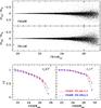 |
Fig. 2 Results of the artificial stars experiments. Upper panels: Difference between the output and input magnitudes of the artificial stars as a function of F814W magnitude. Lower panels: Completeness as a function of F606W magnitude in the inner (r ≤ 1.0′; left panel) and outer (r > 1.0′; right panel) regions of the galaxy. Red continuous curves shows the completeness for stars in the color range of the RGB and the RC, blue dashed curves refer to stars in the color range of the old HB and the YMS (see Fig. 3, below). The blue curves start at F606W = 25.0 because in that color range we produced only artificial stars fainter than this limit, focusing on the study of the completeness in the blue HB region. |
We transformed the star positions from this system into J2000 RA and Dec by fitting a fourth degree polynomial to 5038 stars in common between the ACS catalog and the LBT catalog of Paper I, using the CataPack suite of codes6. The rms of the residual was 0.07″ in both RA and Dec. The positions of the stars in the ACS field with respect to the LBT sample are shown in the upper panel of Fig. 1. In the lower panel of the same figure we zoom on the part of the ACS field containing the center of the galaxy. It is particularly interesting to note that a large number of stars are detected beyond the Rp ≤ 40″ limit of the sample used by J11 for their determination of the SFH. It is beyond that radius, and especially beyond rϵ = 1.5′ where we expect to detect the extended HB of VV124, an obvious tracer of very old (age ≳10 Gyr) and metal-poor populations.
2.1. Artificial stars experiments
To study the completeness of the sample and the photometric uncertainties, we performed a set of artificial star experiments, following the same procedure adopted by Perina et al. (2009, see that paper for a detailed description and references). We produced ≃200 000 artificial stars having 21.0 ≤ F606W ≤ 28.0, with colors in the range covered by the bulk of observed stars, i.e. −0.4 ≤ F606W − F814W ≤ 1.3.
The results of the experiments are presented in Fig. 2. The upper panels show that the photometric accuracy is better than 0.1 mag for F606W ≲ 25.0; a quantitative summary of the results displayed in these panels is presented in Table 1. The lower panels show the completeness factor (Cf) as a function of magnitude for two radial ranges and for two color ranges. At magnitudes fainter than F606W = 25.0, the completeness is slightly worse for blue stars than for red stars. However, even blue stars in the inner radial bin have Cf ≳50% for F606W ≲ 26.5. In the outer radial bin, the same level of completeness is reached at F606W ≃ 27.2.
 |
Fig. 3 Upper panels: CMD of VV124 from the ACS data within (left panel) and outside (right panel) a circle of radius Rp = 40″. The average photometric errors are reported as error bars in the left panel. Lower panels: CMDs in other regions of the ACS field delimited by the ellipses plotted in Fig. 1. The right panel regards a radial region similar to that considered in Paper I to tentatively detect the extended HB population (see their Fig. 9). In all the panels stars are plotted as black points in regions of the CMD with a few stars and as gray squares otherwise, with the scale of gray proportional to the local density of stars in the CMD (lighter tones of gray correspond to higher density). |
Photometric errors from artificial stars experiments.
3. The extended HB of VV124
In the upper lefthand panel of Fig. 3 we show the ACS CMD of VV124 in the same radial range as studied by J11 (Rp ≤ 40″). The two CMDs are very similar, as expected, since they are obtained from the same dataset and with the same photometry package.
The most obvious features are the broad RGB, with the RGB tip located at F814W ~ 21.5, and the red clump (RC) of intermediate/low mass core He burning stars around F814W ~ 25.3. A handful of asymptotic giant branch stars is present on the extension of the RGB above the tip. The obvious blue plume of young main sequence stars (YMS) runs over all the considered magnitude range around F606W − F814W ~ −0.2. The sparse plume protruding from the RGB at F814W ~ 23.5 toward the blue has been identified by J11 as composed of blue loop (BL) stars of metallicity [Fe/H] ~ −0.7; these are the evolved counterpart of the YMS.
J11 noted that the synthetic CMD best reproducing the observations included HB stars reaching colors as blue as V − I ~ F606W − F814W ≃ 0.4 that were not identified in the observed CMD. We note, on the other hand, that it seems possible to discern a blue extension of the HB in our CMD around F814W ~ 25.8 and 0.0 ≲ F606W − F814W ≲ 0.6. This impression is confirmed by the CMD of stars beyond the region studied by J11 displaying an obvious extended HB (upper righthand panel of Fig. 3), with an higher-density portion between F606W − F814W ≃ 0.6 and F606W − F814W ≃ 0.3, and a less populated part reaching F606W − F814W ≃ −0.4.
The extended HB becomes more evident when more external regions are considered, as shown in the lower panels of Fig. 3. This should be partially due to the decreased crowding, which allows to get more accurate photometry, thus decreasing the width of the other CMD sequences that may partially overlap with the HB. However, the most important effect is the decreasing impact of the young MS plume, which contributes to hiding the blue HB near the center of VV124. We show below that, in addition to these observational factors, there is also a genuine population gradient making the HB stars more abundant in the outer regions of the galaxy. The lower righthand panel of the figure shows the CMD in the same radial region where we tentatively detected the extended HB from the LBT data, thus providing a direct confirmation of that finding.
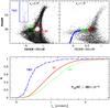 |
Fig. 4 Upper left panel: the adopted selection boxes are plotted on the CMD for rϵ > 0.5′ (the innermost region has been excluded to avoid confusion in the panel). Upper right panel: a synthetic HB population computed from BASTI models, reported to the same distance and reddening of VV124, is superposed to the observed CMD for rϵ > 1.5′. The radial selection is adopted to obtain the cleanest view of the HB. Red HB, RR Lyrae variables, and blue HB are plotted in red, green, and blue, respectively. Lower panel: radial distribution of the various populations selected with the CMD boxes, as indicated by the labels. |
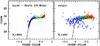 |
Fig. 5 Left panel: CMD of the synthetic stars from the BASTI model shown in Fig. 4 having 25.5 ≤ F606W ≤ 28.0. The meaning of the symbols is the same as in Fig. 4. The continuous line is the corresponding Zero Age HB model, plotted in both panels as a reference. Right panel: simulation of the observation process on the synthetic stars, obtained from the artificial stars experiments (sample with rϵ > 1.5′). Note that the output HB morphology is very similar to the observed one. |
In the upper righthand panel of Fig. 4, we superposed a synthetic HB population, produced from the BASTI theoretical models (Pietrinferni et al. 2004) with the dedicated web tool7, to the observed CMD of the outermost region of VV124 sampled by the ACS data. The synthetic population (1000 stars) have Z = 0.001 (appropriate for the old population of the galaxy, according to Kopylov et al. 2008, Paper I and J11), a mean mass of 0.494 M⊙, and a dispersion σ = 0.2 M⊙, and it has been shifted to the distance and reddening of VV124. This is not intended to reproduce the observed HB but only to provide a sanity check for interpreting of the sequence and to have a hint of the classification of stars within the HB (color-coded according to the classification provided by the model). In particular, it is evident that the galaxy very likely hosts a significant population of RR Lyrae variables, since there are many HB stars in the color range typical of these variables. Clearly their definitive classification as genuine RR Lyrae would need time series photometry, which is not available to us. The detection of such a rich population of candidate RR Lyrae and blue HB stars is fully compatible with the SFH derived by J11, who conclude that ≳90% of the stars were formed between 14 and 10 Gyr ago.
For F606W − F814W ≲ 0.0, the bluest portion of the observed HB seems to depart from the behavior predicted by the models, showing only a modest decline in the mean magnitude with color, while the synthetic population plunges towards much fainter luminosity. This may be from a combination of effects, including imperfect temperature-color transformations in this extreme color regime and photometric errors/ completeness/blending/selection effects due to the proximity of the limiting magnitude level, which becomes brighter for bluer colors. In Fig. 5 we simulate the observational effects on a subsample of the synthetic HB stars. The experiment demonstrates that the apparent mismatch can be fully accounted for by the effects of photometric errors and blending. As a result, most of the stars in the horizontal strip around F606W ~ 26.5 and bluer than F606W − F814W ~ 0.0 are genuine BHB stars (at least for rϵ > 1.5′, where the contamination by YMS stars is negligible), in spite of the apparent mismatch with the raw models8.
The upper lefthand panel of Fig. 4 shows the boxes we adopted for selecting stars on the YMS, in the RC and in the extended HB, to compare their spatial distributions. For the HB we adopted a box covering a relatively narrow color range, approximately matching the one of RR Lyrae variables. This choice was forced by the need to avoid contamination from RC stars on the red side and, above all, from faint YMS stars on the blue side. This would have been particularly problematic since (a) YMS are obviously much more centrally concentrated than older stars, and (b) the YMS blue plume becomes wider and reaches redder colors at faint magnitudes (V ≲ 25), clearly overlapping with the blue HB in the central region. We verified that the actual radial distribution of HB stars bluer than the adopted selection box is fully compatible with a population having the same radial distribution as the HB sample plus a strong contamination of YMS in the innermost ~0.5′. The selected HB sample can therefore be considered as a fair tracer of the old HB population as a whole, including BHB. The selected RC and HB samples should have similar completeness properties, since they have similar magnitudes and colors. To verify this hypothesis we compared the behavior of the completeness as a function of rϵ for the two samples, using our set of artificial stars. It turned out that the two completeness curves are indistinguishable, hence, any observed difference in the radial distribution of RC and HB stars cannot be accounted for by completeness effects.
The cumulative radial distributions of the three selected populations are compared in the lower panel of Fig. 4. In addition to the striking (and already noted) difference between the YMS and the older RC and HB populations, it is clearly revealed that the HB stars have a more extended distribution than do RC stars. A Kolmogorov-Smirnov test gives that the probability that the two samples are extracted from the same parent population is P < × 10-10, thus firmly establishing the significance of the difference. It must be concluded that VV124 displays the classical population gradient observed in all dwarf galaxies, with the older and/or more-metal-poor populations becoming increasingly more abundant at larger radii and younger and/or more-metal-rich being more concentrated toward the center (Harbeck et al. 2001; Bellazzini et al. 2002a, 2005; Tolstoy et al. 2009).
3.1. The color distribution of RGB stars
In Paper I, the comparison of the observed RGB with empirical templates from Galactic globular clusters revealed the possible presence of a small metallicity gradient in the same sense. The analogous comparison, performed with the much more accurate ACS photometry is presented in Fig. 6, to check the findings of Paper I and to verify that the distribution and mean color of RGB stars is compatible with the gradient found with the HB stars. It must be stressed that the following analysis is not intended to provide accurate metallicity estimates, since it is well known that photometric determinations of the metallicity can be affected by serious degeneracies when the underlying age distribution is not well constrained (see Cole et al. 2005; Lianou et al. 2011, and references therein). On the other hand we look for differences in the inner and outer samples of RGB stars that may or may not be in agreement with the observed HB gradient. In the analysis we adopt the global metallicity parameter [M/H] introduced by Salaris et al. (1993) to allow meaningful comparisons between the RGB colors of stellar populations having different α-element abundances (see also Ferraro et al. 1999; Bellazzini et al. 2002a; Salaris et al. 2002).
Figure 6 shows that the fraction of stars spilling to the red of the [M/H] = −1.21 template is indeed greater in the 0.5′ ≤ rϵ < 1.0′ range than at larger distances, even if the amplitude of the color spread is smaller than what is apparent in Paper I. Considering only stars in the range 21.7 ≤ F814W ≤ 23.0 (i.e. the least affected by photometric errors and crowding effects) and enclosed between the bluest and the reddest template, we computed the fraction of stars lying to the red of the [M/H] = −1.21 ridge line. This is 0.29 ± 0.03 in the range 0.5′ ≤ rϵ < 1.0′ and 0.20 ± 0.02 for rϵ ≥ 1.0′. The same result is obtained also if stars with rϵ < 0.5′ are included in the inner bin, and if stars down to F814W = 23.5 are considered. This is very similar to the results obtained in Paper I and in broad agreement with the gradient shown in Fig. 4.
We obtained metallicity estimates for individual stars with F814W ≤ 23.0, by linear interpolation within the templates grid, as in Paper I. The resulting metallicity distributions are quite broad, ranging from the blue limit of the grid, [M/H] = −1.95, to [M/H] ~ −1.0. The mean metallicity in the range 0.5′ ≤ rϵ < 1.0′ is ⟨ [M/H] ⟩ = −1.4, while it is ⟨ [M/H] ⟩ = −1.5 for rϵ ≥ 1.0′. The associated standard deviation, deconvolved from the observational effects, is σ [M/H] ≃ 0.25 dex in both radial bins, also in reasonable agreement with the results of Paper I.
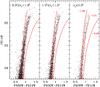 |
Fig. 6 Comparison of the CMDs of VV124 in different (elliptical) radial annuli with the RGB ridge lines for the Galactic globular clusters NGC 6341, NGC 6752 and NGC 104 (from left to right), from the set by Bedin et al. (2005), that provides the templates in the same ACS-WFC VEGAMAG system as our observations. The reddening, distance moduli and metallicities of the clusters are taken from Ferraro et al. (1999), as in Paper I. In the right panel the ridge lines are labeled with the [M/H] value of the corresponding cluster in the Carretta & Gratton (1997) scale (Col. 4 of Table 2 of Ferraro et al. 1999). The radial range of the left panel coincides with the innermost radial range considered in Paper I. |
4. The spatial distributions of H i and young stars
In Fig. 7 we compare the location of those stars identified as YMS with the H i distribution. This comparison clearly shows that, when considered on large scales, there is a very good spatial correspondence between the distribution of the YMS stars and that of the H i, and both show the same asymmetry. Such an overall correspondence is not entirely unexpected, because, after all, stars form from gas. On smaller scales (i.e. less than 100 pc), the spatial correspondence between YMS stars and the H i is not as good, with the peak of the H i somewhat displaced from the YMS stars. This situation is typical for small galaxies, because a good correlation between star formation and H i on large scales and the breakdown of it on smaller scales is observed in many small galaxies (Begum et al. 2006; Roychowdhury et al. 2009).
The close overall correspondence between the YMS and the H i also suggests that the observed kinematics of the H i is also connected to the formation of those stars we now observe on the YMS. As discussed in Paper I, if the H i tail is interpreted as an outflow, the energy output of roughly a dozen OB stars would be enough to drive it. However, an interesting alternative is that the tail corresponds to infall of gas and that VV124 is re-accreting part of the gas that was expelled by the formation of the stars we now see as an old population. That such re-accretion may occur is suggested by some recent simulations (e.g., Sawala et al. 2011), and would also be very consistent with the fact that VV124 has been dormant for a long period of time since the early phase of star formation and has only very recently started to form young stars again. The metallicity of the young stars in VV124 ([Fe/H] ~ −0.7, as estimated by J11 from the observed morphology of the BL) also suggest that, if they formed from the HI gas cloud, this cloud must contain enriched material and hence it consists of re-accreted material.
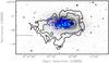 |
Fig. 7 Contours of the total HI image drawn on top of an optical g band image obtained with the LBT, both from Paper I. Contour levels are 5, 10 (black contours), 20 and 50 (white contours) × 1019 cm-2. Blue circles denote the stars with −0.4 < V − I < 0.0 and 23 < I < 25.5 while the cyan circles show the positions of the stars in the same color interval but with I < 23, as if Fig. 1). |
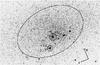 |
Fig. 8 The two candidate clusters (C1 and C2) are indicated on this image of the center of VV124 (from the drizzled F606W image). The circle around C1 has a radius of 2.5″, the one around C2 a radius of 2.0″. The ellipse has the same ellipticity and orientation of the VV124 isophotes and semi-major axis a = 25″. The center of the galaxy is indicated by a cross. |
5. Luminous star clusters in VV124
The zoomed view of the galaxy center shown in Fig. 8 shows that the candidate star cluster identified in Paper I (Cluster 1, C1 hereafter) is indeed largely resolved into stars in the ACS images, hence it is likely a genuine star cluster (see below). On the other hand, the two bright sources to the west of C1 are a background galaxy and a foreground star, respectively. There are several small groups of young stars in this regions that may be possibly classified as open clusters or associations. However, the only other group of size/luminosity comparable to C1 is the one indicated as Cluster 2 (C2) in the figure. C2 appears to coincide with the position of the H ii region identified by Kopylov et al. (2008, by means of a long slit optical spectrum). With the available data it is not possible to establish whether the H ii region is associated to the cluster or it is just a chance superposition.
 ratios for the candidate star clusters and their control fields.
In Sects. 5.1 and 5.2, below, we will study in deeper detail these two small stellar systems. The insight into the physical properties of the clusters is greatly hampered by stellar crowding which is maximized with respect to the surrounding field. Indeed, to reach F814W ~ 26.5 in the very small areas enclosing the clusters, we had to relax the selection on the crowding parameter, accepting stars up to crowd <1.0. In addition, the contamination by field stars provides additional problems to the interpretation of the CMDs. For these reasons, the best we can hope to obtain from the analysis of the clusters CMD are age estimates with uncertainties of order 20%−50%, also due to the uncertainty in the associated metallicity and the systematics associated with uncertainties in the theoretical models (Gallart et al. 2005). However such large age uncertainties translates into uncertainties of 10%−20% in the mass estimates obtained by converting total luminosity into mass (see Perina et al. 2009, 2010, and references therein).
In the following analysis we will try to estimate ages by fitting the cluster CMD with BASTI isochrones, following Perina et al. (2009). As a reference value for the cluster metallicity we assume Z = 0.004, i.e. the mean value estimated by J11 for the young population of VV124. Since the two clusters are clearly associated with this young component, this is by far the best guess on the metallicity of the clusters. While we will present only solutions with Z = 0.004, we have attempted to fit the observed CMDs also with isochrones with metallicity ranging from Z = 0.001 to Z = 0.02 and we found that the Z = 0.004 models always provide the best overall fit. Estimates obtained with the Girardi et al. (2000) isochrones, for comparison, gives age values larger by ~30% that those obtained with BASTI isochrones (hence slightly larger mass estimates), keeping fixed any other parameter. Finally, the good match in color between the MS of the models and of the clusters shows that the reddening value adopted for the whole galaxy is appropriate also for the clusters, indicating they are not affected by additional extinction.
5.1. Cluster 1
In Fig. 9 we compare the CMD in a small area (inner radius = 0.6″, outer radius = 2.5″) centered on C1 with those from identical areas centered on positions symmetric with respect to the center of VV124 and which are used as control fields (CF, see the upper right panel of the figure). It is quite clear that, even if the C1 region has a larger area devoid of measured stars because of the higher crowding associated to the cluster center, the C1 CMD show an excess of MS stars fainter than F814W ≃ 24.5 and, in particular, an obvious excess of BL stars, with respect to all the considered CFs. This is clearly observed even if the analysis is limited to stars with crowd <0.3. In particular in the C1 CMD there are 18 stars lying in the superposed BL selection box, while 3, 5, and 4 are found in the CFE, CFN, and CFW CMDs, respectively. The associated excess of BL stars in C1 with respect to the three CFs is at the 3.3σ, 2.7σ, and 3.0σ level. If we limit to the sample of stars with crowd <0.3, we find 11 stars in the BL box of the C1 CMD, while only 3 stars are found in the CMD of each CF.
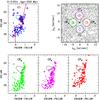 |
Fig. 9 Comparison of the CMDs of the circular annuli around Cluster 1 and three nearby control fields indicated in the upper right panel. In this map the × sign indicates the center of the galaxy. The plotted points correspond to sources having crowd <1.0. In the CMDs, sources with crowd <0.3 are marked by an empty circle concentric to the filled one. An isochrone providing a reasonable fit to the observed CMD is also over-plotted to the C1 CMD (thick red line). A selection box for the BL population is superimposed to each CMD. |
In Table 2 the ratio of stars bluer than F606W − F814W = 0.2 (NB) to the stars redder than F606W − F814W = 0.4 (NR) in the range 24.0 < F814W < 26.0 is shown to be significantly larger (at a >3σ level) in C1 than in any considered CF. Given the regular, compact and roundish appearance of C1 and the obvious excess of young stars found in the C1 area, we conclude that C1 is a genuine star cluster. It is worth noting that the BL and the MS fainter than F814W ~ 24.0 are the only features of the C1 CMD that can be unequivocally attributed to the cluster, as they are significantly over-abundant in the C1 field than in the CFs. On the other hand, one can be tempted to interpret the five stars of the C1 CMD lying in the region F606W − F814W < 0.2 and F814W < 24.0 as very young MS stars associated to the cluster. However this interpretation has no statistical basis, since in the same region there are 3, 1, and 3 stars in CFE,CFN, and CFW, respectively. Hence this handful of bright and blue stars in the C1 CMD is fully compatible with the expectations for the field population. Moreover, we did not find an isochrone that simultaneously matches these very blue stars and the BL population, that is unequivocally associated with C1.
In the upper left panel of Fig. 9 we show also the comparison of the observed CMD of C1 with the isochrone corresponding to our preferred solution. In the age range covered by the young population of VV124, the luminosity of the BL is a very sensitive age indicator (Dohm-Palmer et al. 1997): the BL of C1 is well matched by the adopted isochrone, of age = 250 Myr. Such a young age agrees with the integrated spectra of C1 we presented in Paper I. Following Perina et al. (2009), we associate an uncertainty of ± 50 Myr to our age estimate. All the age estimates we obtained by adopting isochrones of different metallicity (in the range Z = 0.001−0.02) lie within this errorbar.
Observed and derived parameters of cluster C1.
We obtained estimates of the integrated V and I magnitudes from aperture photometry within a circular radius r = 3.0″, corresponding to 15.7 pc9. These, as well as other relevant cluster parameters, are listed in Table 3. While the cluster may be slightly more extended than the adopted radius, this choice should be a reasonable compromise between including most of the cluster light and avoiding strong contamination from the dense field population. The sky level for aperture photometry was estimated in a nearby region to also subtract the contribution from field stars of VV124. From aperture photometry on concentric annuli, and assuming r = 3.0″ as the limiting radius of the cluster, we also obtained a rough estimate of the half-light radius. rh ≃ 1.5″ has been consistently obtained from both the F606W and the F814W images, corresponding to ≃9.5 pc. This is within the range of rh values measured by Barmby et al. (2009) in M31 clusters of similar ages and masses (see below).
The total V luminosity is LV = 6.5 ± 1.0 × 10⁴ L⊙. Assuming  , from a simple stellar population (SSP Renzini & Fusi Pecci 1988) model having Z = 0.004, age = 250 Myr, we obtain M ∗ = 1.2 ± 0.2 × 10⁴ M⊙10. This implies that C1 is significantly brighter than Galactic open clusters of similar ages and it is more massive than Galactic open clusters of any age (Bellazzini et al. 2008b; Perina et al. 2009), except for very few (and much younger) young massive clusters discussed in Figer (2008) and Messineo et al. (2009). On the other hand, it appears very similar in age, mass, and size to the young massive clusters found in relatively large numbers in many star-forming galaxies of any mass (see Larsen & Richtler 1999; Perina et al. 2010; Barmby et al. 2009; Vanzi & Sauvage 2006; Larsen et al. 2011, for references and discussion). In the cluster classification scheme adopted by Larsen & Richtler (2000) and Billett et al. (2002) C1 clearly belongs to the class of regular star clusters (MV < −8.5, see Annibali et al. 2009).
Observed and derived parameters of cluster C2.
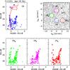 |
Fig. 10 The same as Fig. 9 for Cluster 2. In this case the CFW field is not symmetric with respect to the other CFs, to avoid including a significant portion of C1, whose position is also indicated in the map. |
5.2. Cluster 2
C2 appears more irregular in shape than C1, because it is clearly dominated by a few bright stars. This suggests a younger age than for C1. We performed the same kind of analysis as for C1. The ratio indicates an overdensity of young stars in C2 with respect to all the CFs, albeit at a lower level of significance than in the case of C1 (Table 2). We conclude that C2 is also a likely genuine cluster.
It is very hard to age-date this cluster. If the H ii region is indeed physically associated with C2, the age is constrained to be ≲ 10 Myr, and the three stars brighter than F814W = 21.0 are not cluster BL stars. This is clearly possible since, even if two of them are redder than F606W − F814W = 0.0 and do not have direct counterpart in the CMD of the CFs, this may merely be due to fluctuations inherent in such small numbers of stars.
On the other hand, if these stars are interpreted as genuine cluster BL stars, the age should be greater than the above value and the coincidence with the H ii region must be considered a chance superposition. Unfortunately, the accuracy of the positioning of the H ii region is not sufficient to check the degree of spatial coincidence with C2 on scales smaller than 1″−2″ (see Fig. 2 in Kopylov et al. 2008). Considering the three brightest stars as cluster members, the best fit is obtained with an isochrone of age 30 ± 10 Myr. Given the above discussion, we take this value as an upper limit to the age of C2.
The total V luminosity is LV = 5.4 ± 0.8 × 10⁴ L⊙, the half-light radius is rh ≃ 0.6″, corresponding to ~4 pc (all the estimates as been obtained in the same way as for C1, see above). Assuming  , from an SSP model having Z = 0.004, age = 30 Myr from the BASTI set, we obtain M ∗ ≤ 3.3 ± 0.7 × 10³ M⊙. This is on the high-mass side of the Galactic open cluster distribution, but not out of the range covered by those stellar systems. Also C2 should be included among regular star clusters (Larsen & Richtler 2000; Billett et al. 2002).
6. Summary and conclusions
We have presented a new reduction and analysis of archival HST-ACS images of the isolated dwarf galaxy VV124. A detailed study of the SFH in the innermost regions of the galaxy, from the same data, has been already presented by another group (J11). Here we focused our attention on a few specific issues that have been raised in Paper I and were not addressed in the J11 paper.
-
We provide a clear detection of an extended horizontal branchpopulation. It was shown that HB stars have a spatial distributionthat is less concentrated than the RC population. This stronglysupports the idea that very old and metal-poor stars become moreand more dominant farther from the center of VV124.
-
The near coincidence of the asymmetric sheet of young stars near the center of VV124 and the density peak of the (also asymmetric) associated H i cloud strongly support the idea that the complex kinematics and velocity gradients observed in the gas in Paper I are most likely associated with the dynamics of the star formation episode. It is interesting to note that some of the isolated dwarfs in the simulations by Sawala et al. (2011) lose all their H i at very early times and are able to re-accrete some of the expelled gas at later times. This scenario would be fully consistent with the observed properties of the H i in VV124 and would provide a natural explanation for the long period of quiescence between the early phase of star formation and the very recent sprout of activity that created the sparse population of young MS stars that are currently observed (see J11).
-
We confirm that the candidate cluster identified in Paper I (C1) is a genuine young massive star cluster (see Perina et al. 2010, and references therein). It has an age of ~250 Myr and a total mass of ≃1.2 × 10⁴ M⊙. The cases of such low-mass, early-type dwarf galaxies with massive clusters are quite rare in the Local Group (M98). We identified another likely cluster (C2), significantly younger (age ≤30 Myr) and less massive (M ≤ 3.3 × 10³ M⊙) than C1.
To simulate the observations we proceeded as follows. For each model star plotted in the left panel of Fig. 5, we isolated the subset of artificial stars having input F606W magnitude within ± 0.2 and input color within ± 0.05 of the considered synthetic star. Then we extracted at random one of the selected artificial stars. If the extracted artificial star is not recovered in the output we remove the corresponding synthetic star, thus mimicking the effect of incompleteness. If it is recovered, we compute its output-input difference in magnitude and color and we sum these quantities to the magnitude and color of the synthetic star, thus mimicking the effects of photometric errors and blending (see Bellazzini et al. 2002b, for a similar application). We repeated the experiment several times and verified that the HB morphology in output does not depend on the specific random realization. For an example of detailed modeling of an HB population in a similar context see Monelli et al. (2010, and references therein).
Integrated magnitudes have been transformed from F606W, F814W to V, I using the transformations by Sirianni et al. (2005).
All the BASTI SPSS models adopt a Kroupa (2001) initial mass function (IMF).
Acknowledgments
We warmly thank Andy Dolphin for his precious assistance in the data analysis. We are also grateful to M. Tosi, A. Sollima, and M. Cignoni for critical reading of a draft version of the manuscript. M.B. and S.P. acknowledge the partial financial support for this research by INAF through the PRIN-INAF 2009 grant CRA 1.06.12.10 (PI: R. Gratton). Partial financial support for this study was also provided by ASI through contracts COFIS ASI-INAF I/016/07/0 and ASI-INAF I/009/10/0.
References
- Annibali, F., Tosi, M., Monelli, M., et al. 2009, AJ, 138, 169 [NASA ADS] [CrossRef] [Google Scholar]
- Barmby, P., Perina, S., Bellazzini, M., et al. 2009, AJ, 138, 1667 [NASA ADS] [CrossRef] [Google Scholar]
- Bedin, L. R., Cassisi, S., Castelli, F., et al. 2005, MNRAS, 357 1038 [Google Scholar]
- Begum, A., Chengalur, J. N., Karachentsev, I. D., Kaisin, S. S., & Sharina, M. E. 2006, MNRAS, 365 1220 [Google Scholar]
- Bellazzini, M., Ferraro, F. R., Origlia, L., et al. 2002a, AJ, 124, 3222 [NASA ADS] [CrossRef] [Google Scholar]
- Bellazzini, M., Fusi Pecci, F., Messineo, M., Monaco, L., & Rood, R. T. 2002b, AJ, 123, 1509 [NASA ADS] [CrossRef] [Google Scholar]
- Bellazzini, M., Gennari, N., & Ferraro, F. 2005, MNRAS, 360, 185 [NASA ADS] [CrossRef] [Google Scholar]
- Bellazzini, M., Perina, S., Galleti, S., et al. 2008, Mem. Soc. Astron. Ital., 79, 663 [Google Scholar]
- Bellazzini, M., Beccari, G., Oosterloo, T. A., et al. 2011, A&A, 527, A58 (Paper I) [NASA ADS] [CrossRef] [EDP Sciences] [Google Scholar]
- Billett, O. H., Hunter, D. A., & Elmegreen, B. G. 2002, AJ, 123, 1454 [NASA ADS] [CrossRef] [Google Scholar]
- Carretta, E., & Gratton, R. G. 1997, A&AS, 121, 95 [NASA ADS] [CrossRef] [EDP Sciences] [Google Scholar]
- Cignoni, M., & Tosi, M. 2010, Adv. Astron., article id. 158568 [Google Scholar]
- Cole, A. A., Tolstoy, E., Gallagher, J. S. III, & Smecker-Hane, T. A. 2005, AJ, 129, 1465 [NASA ADS] [CrossRef] [Google Scholar]
- Dohm-Palmer, R., Skillman, E. D., Saha, A., et al. 1997, AJ, 114, 2527 [NASA ADS] [CrossRef] [Google Scholar]
- Dolphin, A. E. 2000, PASP, 112, 1383 [NASA ADS] [CrossRef] [Google Scholar]
- Ferraro, F. R., Messineo, M., Fusi Pecci, F., et al. 1999, AJ, 118, 1738 [NASA ADS] [CrossRef] [Google Scholar]
- Figer, D. F. 2008, in Massive stars as Cosmic Engines, ed. F. Bresolin, & P. A. Crowther, IAU Symp., 250, 247 [Google Scholar]
- Gallart, C., Zoccali, M., & Aparicio, A. 2005, ARA&A, 43, 378 [Google Scholar]
- Galleti, S., Federici, L., Bellazzini, M., Buzzoni, A., & Fusi Pecci, F. 2006, ApJ, 650, L107 [NASA ADS] [CrossRef] [Google Scholar]
- Girardi, L., Bressan, A., Bertelli, G., & Chiosi, C. 2000, A&AS, 141, 371 [Google Scholar]
- Jacobs, B. A., Tully, R. B., Rizzi, L., et al. 2011, AJ, 141, 106 (J11) [NASA ADS] [CrossRef] [Google Scholar]
- Harbeck, D., Harbeck, D., Grebel, E. K., et al. 2001, AJ, 122, 3092 [NASA ADS] [CrossRef] [Google Scholar]
- Kopylov, A. I., Tikhonov, N. A., Fabrika, S., Drozdovsky, I., & Valeev, A. F. 2008, MNRAS, 387, L45 [NASA ADS] [CrossRef] [Google Scholar]
- Kroupa, P. 2001, MNRAS, 322, 231 [NASA ADS] [CrossRef] [Google Scholar]
- Larsen, S. S., & Richtler, T. 1999, A&A, 345, 59 [NASA ADS] [Google Scholar]
- Larsen, S. S., & Richtler, T. 2000, A&A, 354, 836 [NASA ADS] [Google Scholar]
- Larsen, S. S., de Mink, S. E., Eldridge, J. J., et al. 2011, A&A, 532, A147 [NASA ADS] [CrossRef] [EDP Sciences] [Google Scholar]
- Lianou, S., Grebel, E. K., & Koch, A. 2011, A&A, 531, A152 [NASA ADS] [CrossRef] [EDP Sciences] [Google Scholar]
- Mackey, A. D., Huxor, A., Ferguson, A. M. N., et al. 2006, ApJ, 653, L105 [NASA ADS] [CrossRef] [Google Scholar]
- Messineo, M., Davies, B., Ivanov, V. D., et al. 2009, ApJ, 697, 701 [NASA ADS] [CrossRef] [Google Scholar]
- Monelli, M., Gallart, C., Hidalgo, S. L., et al. 2010, ApJ, 722, 1864 [NASA ADS] [CrossRef] [Google Scholar]
- Perina, S., Barmby, P., Beasley, M. A., et al. 2009, A&A, 494, 933 [NASA ADS] [CrossRef] [EDP Sciences] [Google Scholar]
- Perina, S., Cohen, J. G., Barmby, P., et al. 2010, A&A, 511, A23 [NASA ADS] [CrossRef] [EDP Sciences] [Google Scholar]
- Percival, S. M., Salaris, S., Cassisi, S., & Pietrinferni, A. 2009, ApJ, 690, 427 [NASA ADS] [CrossRef] [Google Scholar]
- Pietrinferni, A., Cassisi, S., Salaris, M., & Castelli, F. 2004, ApJ, 612, 168 [NASA ADS] [CrossRef] [Google Scholar]
- Renzini, A., & Fusi Pecci, F. 1988, ARA&A, 26, 199 [NASA ADS] [CrossRef] [Google Scholar]
- Rizzi, L., Held, E. V., Bertelli, G., et al. 2002, in Observed HR Diagrams and stellar evolution, ed. T. Lejeune, & J. Fernandes, ASPCS, 274, 490 [Google Scholar]
- Roychowdhury, S., Chengalur, J. N., Begum, A., & Karachentsev, I. D. 2009, MNRAS, 397, 1435 [NASA ADS] [CrossRef] [Google Scholar]
- Salaris, M., Chieffi, A., & Straniero, O. 1993, ApJ, 414, 580 [NASA ADS] [CrossRef] [Google Scholar]
- Salaris, M., Cassisi, S., & Weiss, A. 2002, PASP, 114, 794 [Google Scholar]
- Sawala, T., Scannapieco, C., Maio, U., & White, S. 2010, MNRAS, 402, 1599 [NASA ADS] [CrossRef] [Google Scholar]
- Sawala, T., Scannapieco, C., & White, S. 2011, MNRAS, in press [arXiv:1103.4562] [Google Scholar]
- Schlegel, D. J., Finkbeiner, D. P., & Davis, M. 1998, ApJ, 500, 525 [NASA ADS] [CrossRef] [Google Scholar]
- Sirianni, M., Jee, M. J., Benítez, N., et al. 2005, PASP, 117, 1049 [NASA ADS] [CrossRef] [Google Scholar]
- Tikhonov, N. A., Fabrika, S. N., Sholukhova, O. N., & Kopylov, A. I., 2010, Astron. Lett., 36, 309 [NASA ADS] [CrossRef] [Google Scholar]
- Tolstoy, E., Hill, V., & Tosi, M. 2009, ARA&A, 47, 371 [NASA ADS] [CrossRef] [Google Scholar]
- Vanzi, L., & Sauvage, M. 2006, A&A, 448, 471 [NASA ADS] [CrossRef] [EDP Sciences] [Google Scholar]
- Weisz, D. R., Dalcanton, J. J., Williams, B. F., et al. 2011, ApJ, in press [arXiv:1101.1093] [Google Scholar]
All Tables
All Figures
|
Fig. 1 Upper panel: stars detected in the ACS images (dark dots) are superposed to the stars from the LBT sample of Paper I (gray dots) in a projected coordinate system centered on the center of VV124 and rotated to have the X axis coincide with the major axis of the galaxy (see Paper I). Only stars brighter than I = 26.5 from the ACS sample have been plotted, for clarity. Lower panel: zoomed view of the central part of the ACS sample in the same coordinate system. Two concentric ellipses of semi-major axis a = 1.0′ and a = 1.5′, with the same orientation and ellipticity of the galaxy isophotes (see Paper I) are overplotted (in white and in black, respectively). The white circle has a radius Rp = 40″, enclosing the region studied by J11. Blue stars lying on the young main sequence (YMS; −0.4 ≤ V − I ≤ 0.0 and I < 25.5, see Fig. 3) are plotted as red filled circles, the brightest ones (having I ≤ 23.0) are encircled in orange. |
| In the text | |
|
Fig. 2 Results of the artificial stars experiments. Upper panels: Difference between the output and input magnitudes of the artificial stars as a function of F814W magnitude. Lower panels: Completeness as a function of F606W magnitude in the inner (r ≤ 1.0′; left panel) and outer (r > 1.0′; right panel) regions of the galaxy. Red continuous curves shows the completeness for stars in the color range of the RGB and the RC, blue dashed curves refer to stars in the color range of the old HB and the YMS (see Fig. 3, below). The blue curves start at F606W = 25.0 because in that color range we produced only artificial stars fainter than this limit, focusing on the study of the completeness in the blue HB region. |
| In the text | |
|
Fig. 3 Upper panels: CMD of VV124 from the ACS data within (left panel) and outside (right panel) a circle of radius Rp = 40″. The average photometric errors are reported as error bars in the left panel. Lower panels: CMDs in other regions of the ACS field delimited by the ellipses plotted in Fig. 1. The right panel regards a radial region similar to that considered in Paper I to tentatively detect the extended HB population (see their Fig. 9). In all the panels stars are plotted as black points in regions of the CMD with a few stars and as gray squares otherwise, with the scale of gray proportional to the local density of stars in the CMD (lighter tones of gray correspond to higher density). |
| In the text | |
|
Fig. 4 Upper left panel: the adopted selection boxes are plotted on the CMD for rϵ > 0.5′ (the innermost region has been excluded to avoid confusion in the panel). Upper right panel: a synthetic HB population computed from BASTI models, reported to the same distance and reddening of VV124, is superposed to the observed CMD for rϵ > 1.5′. The radial selection is adopted to obtain the cleanest view of the HB. Red HB, RR Lyrae variables, and blue HB are plotted in red, green, and blue, respectively. Lower panel: radial distribution of the various populations selected with the CMD boxes, as indicated by the labels. |
| In the text | |
|
Fig. 5 Left panel: CMD of the synthetic stars from the BASTI model shown in Fig. 4 having 25.5 ≤ F606W ≤ 28.0. The meaning of the symbols is the same as in Fig. 4. The continuous line is the corresponding Zero Age HB model, plotted in both panels as a reference. Right panel: simulation of the observation process on the synthetic stars, obtained from the artificial stars experiments (sample with rϵ > 1.5′). Note that the output HB morphology is very similar to the observed one. |
| In the text | |
|
Fig. 6 Comparison of the CMDs of VV124 in different (elliptical) radial annuli with the RGB ridge lines for the Galactic globular clusters NGC 6341, NGC 6752 and NGC 104 (from left to right), from the set by Bedin et al. (2005), that provides the templates in the same ACS-WFC VEGAMAG system as our observations. The reddening, distance moduli and metallicities of the clusters are taken from Ferraro et al. (1999), as in Paper I. In the right panel the ridge lines are labeled with the [M/H] value of the corresponding cluster in the Carretta & Gratton (1997) scale (Col. 4 of Table 2 of Ferraro et al. 1999). The radial range of the left panel coincides with the innermost radial range considered in Paper I. |
| In the text | |
|
Fig. 7 Contours of the total HI image drawn on top of an optical g band image obtained with the LBT, both from Paper I. Contour levels are 5, 10 (black contours), 20 and 50 (white contours) × 1019 cm-2. Blue circles denote the stars with −0.4 < V − I < 0.0 and 23 < I < 25.5 while the cyan circles show the positions of the stars in the same color interval but with I < 23, as if Fig. 1). |
| In the text | |
|
Fig. 8 The two candidate clusters (C1 and C2) are indicated on this image of the center of VV124 (from the drizzled F606W image). The circle around C1 has a radius of 2.5″, the one around C2 a radius of 2.0″. The ellipse has the same ellipticity and orientation of the VV124 isophotes and semi-major axis a = 25″. The center of the galaxy is indicated by a cross. |
| In the text | |
|
Fig. 9 Comparison of the CMDs of the circular annuli around Cluster 1 and three nearby control fields indicated in the upper right panel. In this map the × sign indicates the center of the galaxy. The plotted points correspond to sources having crowd <1.0. In the CMDs, sources with crowd <0.3 are marked by an empty circle concentric to the filled one. An isochrone providing a reasonable fit to the observed CMD is also over-plotted to the C1 CMD (thick red line). A selection box for the BL population is superimposed to each CMD. |
| In the text | |
|
Fig. 10 The same as Fig. 9 for Cluster 2. In this case the CFW field is not symmetric with respect to the other CFs, to avoid including a significant portion of C1, whose position is also indicated in the map. |
| In the text | |
Current usage metrics show cumulative count of Article Views (full-text article views including HTML views, PDF and ePub downloads, according to the available data) and Abstracts Views on Vision4Press platform.
Data correspond to usage on the plateform after 2015. The current usage metrics is available 48-96 hours after online publication and is updated daily on week days.
Initial download of the metrics may take a while.