| Issue |
A&A
Volume 532, August 2011
|
|
|---|---|---|
| Article Number | A29 | |
| Number of page(s) | 29 | |
| Section | Extragalactic astronomy | |
| DOI | https://doi.org/10.1051/0004-6361/201016136 | |
| Published online | 18 July 2011 | |
The discovery and classification of 16 supernovae at high redshifts in ELAIS-S1
The Stockholm VIMOS Supernova Survey II ⋆,⋆⋆
1
Department of Astronomy, Oskar Klein CentreStockholm University, AlbaNova
University Centre,
106 91
Stockholm,
Sweden
e-mail: This email address is being protected from spambots. You need JavaScript enabled to view it.
2
Space Telescope Science Institute, 3700 San Martin Drive, Baltimore, MD
21218,
USA
3
Tuorla Observatory, Department of Physics and Astronomy,
University of Turku, Väisäläntie
20, 21500
Piikkiö,
Finland
4
CNRS, Université de Toulouse, UPS-OMP, IRAP, Toulouse, France
5
Argelander-Institut für Astronomie, Universität Bonn,
Auf dem Hügel 71,
53121
Bonn,
Germany
Received:
12
November
2010
Accepted:
13
May
2011
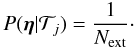
Abstract
Supernova surveys can be used to study a variety of subjects such as: (i) cosmology through type Ia supernovae (SNe), (ii) star-formation rates through core-collapse SNe, and (iii) supernova properties and their connection to host galaxy characteristics. The Stockholm VIMOS Supernova Survey (SVISS) is a multi-band imaging survey aiming to detect supernovae at redshift ~0.5 and derive thermonuclear and core-collapse supernova rates at high redshift. In this paper we present the supernovae discovered in the survey along with light curves and a photometric classification into thermonuclear and core-collapse types. To detect the supernovae in the VLT/VIMOS multi-epoch images, we used difference imaging and a combination of automatic and manual source detection to minimise the number of spurious detections. Photometry for the found variable sources was obtained and careful simulations were made to estimate correct errors. The light curves were typed using a Bayesian probability method and Monte Carlo simulations were used to study misclassification. We detected 16 supernovae, nine of which had a core-collapse origin and seven had a thermonuclear origin. The estimated misclassification errors are quite small, in the order of 5%, but vary with both redshift and type. The mean redshift of the supernovae is 0.58. Additionally, we found a variable source with a very extended light curve that could possibly be a pair instability supernova.
Key words: supernovae: general
Based on observations collected at the European Organisation for Astronomical Research in the Southern Hemisphere, Chile, under ESO programme ID 167.D-0492.
Figures 6–8, 10–12 and Appendix A are available in electronic form at http://www.aanda.org
© ESO, 2011
1. Introduction
During the last couple of decades supernovae have been shown to be powerful probes of both cosmology and star formation in high-redshift galaxies. A number of surveys with various scientific goals have been conducted and proposed. Most of them have in common that multiple imaging epochs are used to detect the supernovae. In some cases the surveys also contain spectroscopic follow-up observations of the detected candidates. The spectroscopic information makes it possible to easily characterise the detected supernovae and to measure redshifts, but this comes at the cost of added telescope time. Whole-sky supernova surveys have already started, e.g., Pan-STARRS1 (Young et al. 2008) and PTF (Rau et al. 2009), and several more are being planned, e.g., SkyMapper and LSST. With the large number of expected supernovae it will not be feasible to obtain spectra for all of them. Photometric techniques will thus be required to characterise the detected sources.
Core-collapse supernovae (CC SNe) are the result of a massive star ending its life in an energetic explosion (see, e.g., Smartt 2009). Because the lifetimes of these massive stars are short, their presence signals that active star-formation is taking place in the host galaxy. The star-formation rate density for a cosmic volume, defined by the redshift range and field size, can be derived from the core-collapse supernova rates by making an assumption on how many stars out of the current star forming population that explode. This method provides an independent tracer of the star-formation history of the universe and has been used by Dahlen et al. (2004b); Botticella et al. (2008); Bazin et al. (2009). While Li et al. (2011a) also provide a local supernova rate, their big sample of SNe is also used to study the host galaxy properties and connections to supernova subtype. Most of these surveys target low-redshift SNe (z ≲ 0.3), but with deep enough observations the technique also works at higher z (e.g. Dahlen et al. 2004b). For this kind of projects it is important that the observations are obtained as a “blind” survey to limit the selection effects.
The use of thermonuclear (Ia) supernovae as standardisable candles has been instrumental in measuring cosmological parameters for the ΛCDM concordance cosmology (e.g. Astier et al. 2006; Riess et al. 2007; Amanullah et al. 2010; Wood-Vasey et al. 2007; Kessler et al. 2009). The systematic errors resulting from the determination of the distance modulus for thermonuclear supernovae have been extensively studied and minimised. To achieve the precision needed to pinpoint cosmological parameters, it is necessary to obtain spectra for the supernovae. Despite the amount of work made on calibrating the distance modulus relation, the underlying physics of thermonuclear supernovae is still partly unknown. In particular, the type of progenitor system that gives rise to the supernovae is uncertain; see, e.g., Ruiter et al. (2009) for a discussion of the different possibilities. One way of putting constraints on progenitor models is to study the delay times of thermonuclear supernovae (i.e., the time between formation of the progenitor star and the supernova explosion). The rate of thermonuclear supernovae compared to either the global (Dahlen et al. 2004b) or the local (Sullivan et al. 2006; Totani et al. 2008; Maoz & Badenes 2010) star formation history can provide estimates on the delay time distribution even without observed spectra of the supernovae. A number of surveys targeting Ia SNe in galaxy clusters have also been undertaken (Sharon et al. 2010; Barbary et al. 2010). Recently, Dilday et al. (2010) presented an accurate measurement of the z ~ 0.1 thermonuclear SN rate from the Sloan Digital Sky Survey II Supernova Survey.
A major challenge to all intermediate- and high-redshift CC SN searches is how to take into account the effects of SNe missed owing to large host galaxy extinctions. Mattila et al. (2007) and Kankare et al. (2008) present supernovae found in the nuclear regions of luminous infrared galaxies (LIRGs) by using infrared adaptive optics imaging. These types of searches are important to constrain the numbers of supernovae lost in LIRGs, in which most of the massive stars are formed at intermediate and higher redshifts (Magnelli et al. 2009).
Typing of supernovae using broad band colours in multiple epochs has been demonstrated to work by several authors (e.g., Barris & Tonry 2004; Johnson & Crotts 2006; Kuznetsova & Connolly 2007; Poznanski et al. 2007a; Sako et al. 2008). The application of the codes vary, in some cases the codes are used mainly to reject core-collapse SNe from the follow-up target lists of cosmological Ia surveys, but in others the codes are used as the only way of typing SNe without spectra. Most of the codes use template-fitting methods where a number of k-corrected thermonuclear and core-collapse SN light curves are compared to the observed light curve and colour evolution. The simplest way of doing this fitting is through χ2 fitting. However, there are some problems with this approach because it does not allow prior information on, e.g., redshifts and peak luminosity to be used to full extent. Kuznetsova & Connolly (2007) introduced a Bayesian approach to supernova typing where probability distributions for the parameters could be used as priors. Lately, Bayesian methods have been further developed by Rodney & Tonry (2009), where “fuzzy” templates are used to improve classification of SNe with non-standard light curves. With this method the templates are assigned an uncertainty that enters into the likelihood calculations, which improves the classification quality of SNe with non-standard light curves. Recently, Kessler et al. (2010a) presented the results of a supernova classification challenge, where a common sample of supernova light curves was typed by different codes. Their results indicate that Bayesian typing codes are competitive and give reliable type determinations.
The Stockholm VIMOS Supernova Survey (SVISS) is a multi-band (R + I) imaging survey aiming to detect supernovae at redshift ~0.5 and derive thermonuclear and core-collapse supernova rates. The supernova survey data were obtained over a six-month period with VIMOS/VLT (LeFevre et al. 2003). Melinder et al. (2008) describe the supernova search method along with extensive testing of the image subtraction, supernova detection and photometry. In this paper we report the discovery of 16 supernovae in one of the search fields of the survey and provide light curves along with type classifications for them. We will present the supernova rates and conclusions to be drawn from them in a future paper (Melinder et al., in prep.).
The first part of the paper contains a description of the data set and the methods used to reduce it. In Sect. 3 we describe the supernova typing method and the template supernova light curves. Section 4 contains a description of how the simulations of supernovae have been set up and offers the results from extensive testing of the typing method. Finally, we present the results and possible implications in Sect. 5 and conclude by discussing and summarising the results in Sect. 6. The Vega magnitude system and a standard ΛCDM cosmology with {h0,ΩM,ΩΛ} = {70,0.3,0.7} have been used throughout the paper.
2. The data
2.1. Observations
The data were obtained with the VIMOS instrument (LeFevre et al. 2003) mounted on the ESO Very Large Telescope (UT3) at several epochs during 2003−2006. The VIMOS instrument has four CCDs, each 2k × 2.4k pixels with a pixel scale of 0.205″/pxl, covering a total area of 4 × 56 sq. arcmin. The SVISS observations were obtained in two fields, covering parts of the Chandra Deep Field-South (Giacconi et al. 2001) and the ELAIS-S1 field (La Franca et al. 2004). The observations in the ELAIS-S1 field were obtained in five broad band filters (U, B, V, R and I) centred at α = 00:32:13, δ = −44:36:27 (J2000). The data used in this paper are only from the ELAIS-S1 observations, the CDF-S observations will be presented in a subsequent paper.
The supernova search filters are R and I, with roughly twice the exposure time in I compared to R. Observations in these filters have been divided into one reference epoch (henceforth epoch 0), seven search epochs and one control epoch. The images used to construct the reference epoch were obtained in August 2003, the search epoch images were obtained from July 2004 to January 2005, while the control epoch was taken in January 2006. The search epochs were separated by roughly one month.
Overview of the ELAIS-S1 observations.
The UBV observations were obtained at several different epochs during the time period 2004−2006. Details on the data reduction and calibration of the UBV data along with a galaxy catalogue for the field will be presented in Mencía-Trinchant et al. (in prep.). In the present paper the UBV observations have only been used to calculate photometric redshifts for supernova host galaxies.
Table 1 contains the specifications of the different epochs and parts of the data. It is worth noting that the quality of data is very good overall with median seeing of 0.76″ and 0.68″ in R/I, respectively, and all search epochs have seeing below 0.9″. As can be seen in the table, the observations are also very deep, with mean 3σ limiting magnitudes of 26.8 and 26.3 in R and I, respectively. In Dahlen et al. (2008) the 50% detection efficiency magnitude of the survey in the F850LP filter is given, converting this to our magnitude system we obtain mI ~ 26.5. This magnitude can be compared to our 3σ limits, based on the findings in Paper I; the depth is thus quite similar. The search for variable objects in the Subaru/XMM-Newton Deep Survey (Morokuma et al. 2008; Totani et al. 2008) has a limiting magnitude of mI ~ 26.0, again converted to our magnitude system. Compared to other SN surveys, our data set is thus among the deepest ever obtained, although smaller in field size than others.
2.2. Data reduction of the R and I observations
The data were reduced using a data reduction pipeline written in MIDAS scripting language for SVISS developed by our team. Each image was bias-subtracted using an epoch master bias frame constructed by median-combining >10 bias frames. Flatfield calibration data were obtained for each night in both filters and all science data were flatfielded using high signal-to-noise stacked frames. Cosmic-ray rejection routines were used to detect possible cosmic rays, but no automatic corrections were applied. Parts of images with suspected cosmic rays were manually inspected and pixels with cosmic ray contamination were flagged. Atmospheric extinction corrections were applied to the images using tabulated extinction coefficients from the ESO quality control web pages. The images were also normalised to counts per second. A bad pixel mask was produced for each of the images, containing vignetted (<5% in most cases), saturated and cosmic ray flagged pixels.
The VIMOS I band suffers from quite severe effects of fringing (see Berta et al. 2008 for a detailed description of fringing for the VIMOS instrument), and care has to be taken to successfully remove these. We constructed a fringe map for each observation night by median-combining the non-aligned science frames and rejecting bright pixels by a standard sigma-rejection routine. To make this possible, the observations were made with a dithering scheme that was optimised to avoid having individual science frames target the same area on sky. For some nights it was necessary to make two fringe maps owing to sky-brightness variations during the night. We did not need to use any masking or smoothing on the resulting fringe maps, there were very few extremely bright sources in our field (causing optical ghosts, as mentioned by Berta et al. 2008) and the noise levels were insignificant compared to the individual frames. The fringe map was then subtracted from each of the flatfielded science frames. Finally, all of the science frames were manually inspected, some frames were removed because of vignetting and/or poor seeing (see Table 1 for the total exposure time used in each epoch).
The good quality frames for each epoch were registered to a common pixel coordinate system using a shift- and rotate-transform (yielding a typical rms of ~0.1 pixels or 0.02″). The registered frames were then median combined. The bad pixel maps for each individual image were also registered and summed, yielding an exposure time map for each epoch. Some pixels (<0.2% in the reference epoch) had an exposure time of zero, i.e., none of the individual frames contained useful data for that pixel. These pixels were flagged in the combined science frames.
Each of the combined epoch images were photometrically calibrated using ~50 secondary photometric standards in the field. The calibrated photometry for these stars was obtained from stacked one-night images from nights where standard-star observations were available. The secondary standard sources were selected by requiring a signal-to-noise ratio of at least 100 and a stellar-like point spread function (PSF). The sources were also required to be isolated in the single-night frame with no visible neighbours within a 10 × FWHM (full width at half maximum) radius. The photometry of the primary and secondary standards was obtained with IRAF/phot using an aperture size of 10 × FWHM (with aperture correction). The resulting zeropoint errors for each epoch are ≲0.02 mag, but it should be noted that all epoch images are scaled to the reference epoch zeropoint in the subtraction procedure.
2.3. Supernova detections and photometry
In Melinder et al. (2008), henceforth Paper I, we presented our supernova detection method, which is explained there in detail. We used IRAF/PYRAF scripts that were run in sequence and proceeded as follows: (i) accurate image alignment over the entire frame; (ii) convolving the better seeing image to the same PSF size and shape as the poorer seeing image, using a spatially varying kernel; (iii) subtracting the images; (iv) detection of sources in the subtracted frames, using both source detection software and naked-eye detection; (v) photometry and construction of light curves of the detected transients.
All search epochs were aligned to the pixel coordinate system of the reference epoch using the geomap/geotran tasks in IRAF/PyRAF. We found that the shift- and rotate-transform used when registering the individual frames was not good enough for registering the search images to the reference image. This is likely caused by changes in the geometry (e.g., differential refraction, changes in flexure of the telescope) of the frames over the time period our observations were obtained. To perform the registration at sub–pixel accuracy, we used a general transform that allows for shifts, rotations, shear, and pixel scale changes in the image being aligned. The reference sources for registration were bright, point-like objects in the field (approximately 100 sources were used). The resulting standard deviations for the geometrical transforms were smaller than 0.1 pixels for all epochs.
Convolution to a common PSF was made with the ISIS 2.2 code (Alard & Lupton 1998; Alard 2000). A convolution kernel was computed by comparing a number of reference sources in the two images. The better seeing image (i.e., the image with smaller PSF width) was then convolved and scaled to match the photometry of the unconvolved image; the convolved frame was either the reference or the search frame. A background variation between the frames was also computed and compensated for. The selection of suitable image subtraction parameters for our dataset was investigated in Melinder et al. (2008). Finally, the reference epoch was subtracted from the search epoch and exposure time maps for the images were combined to make a weight map for the subtracted frame.
2.3.1. Source detection
Source detection was made in the subtracted frames using SExtractor (SE, Bertin & Arnouts 1996) to obtain an initial source list. Separate detection was made in each epoch and filter, except in the very last epoch (sources discovered in the last epoch would only have one point on the light curve and thus automatically fail our selection criterion, see Sect. 2.3.2). The detection parameters for SE were set at a quite liberal level to make sure that no SN candidates were missed (i.e., this detection threshold accepts sources at a lower signal-to-noise level than the rejection criteria, see Sect. 2.3.2). Furthermore, the weight maps for the subtracted frames were used in source detection to lower the number of spurious detections. Using the weight maps reduced this number by about 20%, primarily close to the edges of the frames.
The number of detections in a single subtracted frame is typically in the order of 100 times the expected number of true varying sources. This is consistent with the findings of other supernova surveys using similar techniques (e.g. Miknaitis et al. 2007). Most of these spurious detections are spurious subtraction residuals. About 50% of the spurious sources were then rejected, most of these by requiring that true sources must be present in both the R and I filter at the given epoch. Spurious sources close to saturated stars and image defects were also removed; the total number of candidates for all the epochs remaining after this initial rejection procedure was ~1500. Most of them are spurious detections related to subtraction residuals of bright galaxies that are present in both filters. In Sect. 5 we show how constraints on the light curve and supernova typing can be used to safely reject the remaining spurious detections.
2.3.2. Photometry
Photometry on the detected sources was made using the IRAF daophot package. The PSF photometry was performed on all detected candidates using the task allstar. We also tried using aperture photometry with aperture corrections computed from the original worse seeing image, using the IRAF task phot. This does give fairly good results, but seems to be more susceptible to residual flux from the background galaxies than the PSF photometry, thus giving larger errors (both statistical and systematic) in general.
In Paper I we found that the photometric uncertainties estimated by daophot/phot were underestimating the true noise by a factor of two or more. The two main reasons for this are that (i) the pixels in the subtracted image will be positively correlated owing to the convolution made in the image matching step; (ii) the sky noise is estimated in a region outside of the host galaxy, thus not taking subtraction residuals properly into account. Therefore, we used simulations to obtain reliable error estimates. By simulating SNe at different brightness in each epoch and finding the scatter in their measured magnitudes, we obtained an estimate of the true photometric error for each point on the SN light curve.
The simulations also allowed us to check the photometry for possible systematic errors. In Paper I we discuss the discovery of a small systematic flux offset (~10% at the 3σ limiting magnitudes, lower for brighter sources) in subtracted frames. This offset is not present in all epochs/filters and changes between epochs. We can calculate this offset from the simulations and correct the photometry for this effect in the epochs where it is needed.
R and I light curves are then put together for the 1459 sources remaining after automated detection in the subtracted frames. We rejected spurious detections by requiring the candidates to be brighter than the 3σ limiting magnitudes (see Table 1) in (i) the detection epoch and the subsequent epoch and (ii) both the R and I filters. With this rejection criterion the number of supernova candidates decreased to 115. At this point we are reasonably certain that no true supernova candidates have been dropped (unless they were too faint to fulfil the rejection criterion), but there is likely still a number of spurious detections remaining. In some cases subtraction residuals will appear at the same location in both filters and in multiple epochs (e.g., very bright galaxies).
2.4. Host galaxy redshifts
Using the full set of UBVRI observations, we calculated photometric redshifts for the supernova host galaxies. We used a template-fitting method with the mean galaxy luminosity function as a Bayesian prior, see Dahlen et al. (2010) and Dahlén et al. (2004a). We used 16 SEDs (spectral energy distributions) that were constructed by interpolating between four empirical templates (E, Sbc, Scd and Im galaxy types) from Coleman et al. (1980) and two starburst-galaxy templates from Kinney et al. (1996). For the supernova host galaxies we used photometry from the stacked UBV images, but excluding frames obtained during the time period when the supernova is detectable. For the I and R images we used the reference epoch images. These considerations ensure that the supernova light does not affect the determination of the photometric redshifts.
In our observed subsection of the ELAIS-S1 field only two galaxies have known spectroscopic redshifts. This means that calibration and validating of the photometric redshifts is not straightforward. We obtained archive UBVRI data of the Hubble Deep Field-South (HDF-S) observed with the VIMOS instrument. The HDF-S has been observed extensively with spectroscopy and we found 280 sources with spectroscopic redshifts ranging from z ~ 0 to z ~ 3.5 that are also found in the VIMOS HDF-S observations (Vanzella et al. 2002; Rigopoulou et al. 2005; Glazebrook et al. 2006). We reduced and analysed the HDF-S photometric data in the same way as the ELAIS-S1 data set. The photometric calibration was also made in the same way (including corrections for galaxtic extinction) as for the ELAIS-S1 observations.
Comparing the spectroscopic redshifts to the photometric redshifts obtained from the imaging data, we find a redshift uncertainty of δz = 0.085 ∗ (1 + z) and a frequency of catastrophic failures (defined as |zphot − zspec| > 0.3) of 9%. Because the instrument and filters are the same, the analysis is made in exactly the same way and the depth of the imaging data is comparable, we assume that the uncertainties of the SVISS redshifts are the same as the uncertainties determined for this dataset. The uncertainty of the redshift determination was taken into account in the supernova typing, see Sect. 4.1. The photometric redshift technique and calibrations of it as applied to our data set will be presented in greater detail in Mencía-Trinchant et al. (in prep.).
At first, the host galaxies were identified as the closest galaxies to the SNe in terms of angular separation. But when the redshift information was also considered, it became clear that some of the identified hosts were at unrealistical redshifts, either making any SNe in them too faint to be detectable or too bright compared to our templates. Instead of angular separation we therefore used the photometric redshift information and chose the closest galaxy in terms of physical distance. With this method we were able to identify hosts for 13 of the SNe. For one of these (SN309) the chosen host was not the closest galaxy in angular distance. Identifying hosts for the SNe in this way is of course not unproblematic, there is a risk of selecting an incorrect host galaxy. We did not try to estimate the percentage of misidentifications, but we reran the typing for all 13 SNe using a flat redshift prior and, in relevant cases, also with redshift priors based on other closeby galaxies. The result of these tests is that none of these SNe change main type and that the changes in redshift are small. We conclude that host misidentification has only little effect on the main results of this paper.
For the remaining three supernovae (SN-14, SN-31 and SN-261) there are no nearby galaxies with redshifts that are consistent with hosting a SNe with the observed light curve. For these three SNe we ran the typing code without photometric redshifts supplied, thus using a flat prior on the redshift. This is also discussed in more detail in Sect. 5.2. More information on the host galaxy identification and properties of these galaxies will be presented in an upcoming paper (Mencía Trinchant et al., in prep.).
3. Supernova typing method
Our typing method relies on a Bayesian template-fitting algorithm. The use of prior
probabilities and Bayesian marginalisation makes it possible to include previously known
information on the different supernova types in the fitting technique while avoiding
over-fitting. The goal of the method is to find the most likely supernova type
( )
given an observed light curve ({F} ) of a supernova candidate. The
description of the Bayesian method follows Kuznetsova
& Connolly (2007), although the notation and scope is slightly different.
All calculations were made in a parallelised FORTRAN 90 code using double precision.
)
given an observed light curve ({F} ) of a supernova candidate. The
description of the Bayesian method follows Kuznetsova
& Connolly (2007), although the notation and scope is slightly different.
All calculations were made in a parallelised FORTRAN 90 code using double precision.
Formally we want to find the type that maximises the probability
 ,
where
,
where ![Mathematical equation: \hbox{$j=[1,...,N_{\mathcal{T}}]$}](/articles/aa/full_html/2011/08/aa16136-10/aa16136-10-eq47.png) refers to the different types and
i = [1,..., Ndp]
to the points on the observed light curve. Nine supernova types (Ia, Iafaint,
Ia91bg−like Ia91t−like, Ibcnormal, Ibcbright,
IIn, IIL and IIP) were considered. The total number of data points
(Ndp) is given by the product of the number of filters
(Nfilters) and the number of observation epochs
(Nep). The SVISS observations were made in two filters
(R and I) and in seven epochs, thus
Ndp = 14 in this work. The probability
cannot be calculated directly; using Bayes’ theorem we can rewrite the probability:
refers to the different types and
i = [1,..., Ndp]
to the points on the observed light curve. Nine supernova types (Ia, Iafaint,
Ia91bg−like Ia91t−like, Ibcnormal, Ibcbright,
IIn, IIL and IIP) were considered. The total number of data points
(Ndp) is given by the product of the number of filters
(Nfilters) and the number of observation epochs
(Nep). The SVISS observations were made in two filters
(R and I) and in seven epochs, thus
Ndp = 14 in this work. The probability
cannot be calculated directly; using Bayes’ theorem we can rewrite the probability:
 (1)
(1) is the probability of obtaining the light curve data
{Fi} for a given supernova type
is the probability of obtaining the light curve data
{Fi} for a given supernova type
 .
.
 contains all prior information on the supernova model light curve for the specific type.
When Bayes’ theorem is used in this fashion, we implicitly assume that the set of supernova
types is complete, i.e., all supernova candidates must be one of the considered types. For
sufficiently peculiar supernovae, and non-supernovae, Eq. (1) will not give valid probabilities. In Sect. 4.3 we describe how we use measures of goodness-of-fit to purge
candidates with light curves that are too dissimilar from the model curves.
contains all prior information on the supernova model light curve for the specific type.
When Bayes’ theorem is used in this fashion, we implicitly assume that the set of supernova
types is complete, i.e., all supernova candidates must be one of the considered types. For
sufficiently peculiar supernovae, and non-supernovae, Eq. (1) will not give valid probabilities. In Sect. 4.3 we describe how we use measures of goodness-of-fit to purge
candidates with light curves that are too dissimilar from the model curves.
For each of the nine supernova types we created template light curves using absolute
magnitude (MB) light curves and SEDs, which are
described in more detail in Sects. 3.3 and 3.3.6. We used four parameters that uniquely define the
light curve for a given type: (i) MB the
absolute rest-frame B band magnitude at peak; (ii) z, the
redshift of the supernova; (iii) t, the time difference between the
explosion date for the model and the first observational epoch; (iv)
{RV,E(B − V)} = η;
extinction in the host galaxy. We denote the template light curves by
{fi,j}
 (2)and because these
parameters uniquely define the light curve for a specific type, we may rewrite
as
P({Fi}|{fi,j(MB,z,t,η)})
and
as
(2)and because these
parameters uniquely define the light curve for a specific type, we may rewrite
as
P({Fi}|{fi,j(MB,z,t,η)})
and
as  .
.
We define the likelihood function for each supernova type:  (3)The
probability that a supernova with a template light curve
fi,j will have an observed light curve,
{Fi} , is
(3)The
probability that a supernova with a template light curve
fi,j will have an observed light curve,
{Fi} , is  (4)where each observational
data point is allowed to fluctuate according to Gaussian statistics (the widths of the
distributions are given by the observational errors,
δFi). It should be noted
that the photometric quantities in this expression are in units of flux (counts/sec).
Non-detections are included in the analysis as data points with zero flux and with an error
given by the 1σ limiting fluxes.
(4)where each observational
data point is allowed to fluctuate according to Gaussian statistics (the widths of the
distributions are given by the observational errors,
δFi). It should be noted
that the photometric quantities in this expression are in units of flux (counts/sec).
Non-detections are included in the analysis as data points with zero flux and with an error
given by the 1σ limiting fluxes.
The ,
or equivalently  ,
prior contains all prior information on the parameters for a given template. We assume that
the parameters are independent and can thus factorise the prior:
,
prior contains all prior information on the parameters for a given template. We assume that
the parameters are independent and can thus factorise the prior:  (5)The
individual parameter priors are described in the next section. The remaining prior,
contains information on whether a specific supernova subtype is more likely than others. The
relative rates of supernova subtypes are not well constrained at high redshifts. Therefore,
we assume that the prior probability for a supernova candidate to be of a certain subtype is
equal for all the types (i.e., a flat prior),
(5)The
individual parameter priors are described in the next section. The remaining prior,
contains information on whether a specific supernova subtype is more likely than others. The
relative rates of supernova subtypes are not well constrained at high redshifts. Therefore,
we assume that the prior probability for a supernova candidate to be of a certain subtype is
equal for all the types (i.e., a flat prior),
 (6)There are more
priors/parameters that could have been used to construct the template prior. Including more
prior information will of course affect the typing and can make it more accurate. For this
to work, the parameter in question needs to have a known probability distribution (or at
least a valid range of values). It should be noted that adding more priors will cause the
computation time of the typing to increase by a factor equal to the number of steps used for
the probability distribution. Our choice of four priors is thus based on a compromise
between limiting computing time and choosing parameters with well-known distribution on one
hand and typing accuracy on the other. Other authors have used additional or a different set
of priors. Kuznetsova & Connolly (2007)
include prior information on stretch in their typing code, using a Gaussian distribution
with mean and width from observations. In our code we use thermonuclear supernova templates
with different stretch to account for this variance. The inclusion of a colour uncertainty
to the templates can also be described in terms of an additional prior, this has been used
by, e.g., Poznanski et al. (2007a). We do not have
colour uncertainty in our typing, instead we choose to use more templates that have
different colour evolution.
(6)There are more
priors/parameters that could have been used to construct the template prior. Including more
prior information will of course affect the typing and can make it more accurate. For this
to work, the parameter in question needs to have a known probability distribution (or at
least a valid range of values). It should be noted that adding more priors will cause the
computation time of the typing to increase by a factor equal to the number of steps used for
the probability distribution. Our choice of four priors is thus based on a compromise
between limiting computing time and choosing parameters with well-known distribution on one
hand and typing accuracy on the other. Other authors have used additional or a different set
of priors. Kuznetsova & Connolly (2007)
include prior information on stretch in their typing code, using a Gaussian distribution
with mean and width from observations. In our code we use thermonuclear supernova templates
with different stretch to account for this variance. The inclusion of a colour uncertainty
to the templates can also be described in terms of an additional prior, this has been used
by, e.g., Poznanski et al. (2007a). We do not have
colour uncertainty in our typing, instead we choose to use more templates that have
different colour evolution.
3.1. The parameter prior distributions
Properties of the supernova photometric templates.
Each of the four parameters has an associated probability distribution function. The parameter priors on the right hand side of Eq. (5) are given by the respective probabilities.
The prior on the peak absolute B magnitude is given by  (7)where
⟨ MB ⟩ is the mean peak magnitude for a
given supernova type (see Table 2 and the
discussion in Sect. 3.3),
σM is the dispersion of the mean magnitude and
ΔM is the numerical step size. Assuming the peak magnitudes to be
normally distributed around the mean is consistent with observations, cf. Richardson et al. (2002) and Richardson et al. (2006). The range in peak absolute magnitudes
considered is given by
[⟨ MB ⟩ −2σM, ⟨ MB ⟩ + 2σM]
for each subtype and the numerical step size used is ~0.02−0.04.
(7)where
⟨ MB ⟩ is the mean peak magnitude for a
given supernova type (see Table 2 and the
discussion in Sect. 3.3),
σM is the dispersion of the mean magnitude and
ΔM is the numerical step size. Assuming the peak magnitudes to be
normally distributed around the mean is consistent with observations, cf. Richardson et al. (2002) and Richardson et al. (2006). The range in peak absolute magnitudes
considered is given by
[⟨ MB ⟩ −2σM, ⟨ MB ⟩ + 2σM]
for each subtype and the numerical step size used is ~0.02−0.04.
The redshift prior used is either a Gaussian or a flat distribution, depending on whether
the host galaxy has a valid photometric redshift available or not. The mean,
zp and width, δz of the Gaussian
distribution is given by the photometric redshift fitting of the host galaxy (see
Sect. 2.4 and Mencía-Trinchant et al., in prep.).
The redshift of the supernova is independent of the supernova type, thus we may write
 and obtain
  (8)Δz is
the numerical step size, similar to ΔM in Eq. (7). The flat redshift prior is given by
(8)Δz is
the numerical step size, similar to ΔM in Eq. (7). The flat redshift prior is given by
 (9)where
[zl,zu] is the
lower and upper limits of the redshift interval considered. For both distributions we used
a numerical step size of 0.02 in redshift and a redshift interval given by
[zl,zu] = [0.0,2.0].
(9)where
[zl,zu] is the
lower and upper limits of the redshift interval considered. For both distributions we used
a numerical step size of 0.02 in redshift and a redshift interval given by
[zl,zu] = [0.0,2.0].
The probability of a given time difference is assumed to be equal for all time
differences between t1 to t2. The
time difference probabilities do no depend on the type,
 ,
and the prior is
,
and the prior is  (10)where Δt
is the numerical step size and Nt the number
of steps. We used Δt = 1 day throughout this work. The time difference
interval considered is given by
[t1,t2] = [− 136,142],
this interval is chosen based on the time difference between our search epochs and that we
require supernova candidates to be observed in at least two subsequent epochs.
(10)where Δt
is the numerical step size and Nt the number
of steps. We used Δt = 1 day throughout this work. The time difference
interval considered is given by
[t1,t2] = [− 136,142],
this interval is chosen based on the time difference between our search epochs and that we
require supernova candidates to be observed in at least two subsequent epochs.
The extinction models considered are two Cardelli laws (Cardelli et al. 1989) with RV = 2.1
and 3.1 and the Calzetti law (Calzetti et al. 2000)
with RV = 4.05. Some authors have reported
indications of steep extinction laws for supernovae (e.g. Goobar 2008), this motivates the inclusion of the
RV = 2.1 law. The Calzetti law is
normally used in star-forming galaxies and is therefore a reasonable assumption for
core-collapse supernovae. However, all extinction laws are considered for any given type.
The second parameter for the extinction is the colour excess,
E(B − V), the range of excess
considered is 0.0 ≤ E(B − V) ≤ 0.6 with
step size of 0.1. The total number of combinations of the different extinction laws and
values of E(B − V)
(η) is Next = 21. We assume
a flat prior that does not depend on the type under consideration and arrive at
 (11)We performed tests on
simulated and real data that indicate that the typing is fairly insensitive to changes of
the extinction prior range. Using a higher maximum extinction or a different step size
does not change the type of any of the observed SNe (see Sect. 5).
(11)We performed tests on
simulated and real data that indicate that the typing is fairly insensitive to changes of
the extinction prior range. Using a higher maximum extinction or a different step size
does not change the type of any of the observed SNe (see Sect. 5).
3.2. Determining the most likely supernova type
When trying to find the most likely supernova type, the four parameters are all nuisance
parameters, we marginalize the likelihood function over the four parameters to get the
summed likelihood function, or in Bayesian terms, the evidence:  (12)Combining
this, we arrive at the following formula for the evidence (given that photometric redshift
for the host is available):
(12)Combining
this, we arrive at the following formula for the evidence (given that photometric redshift
for the host is available): 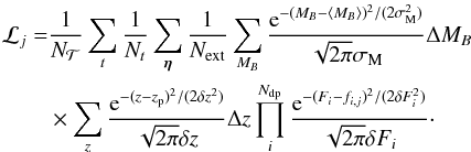 (13)The
probability
is then equal to the relative evidence for each supernova type,
(13)The
probability
is then equal to the relative evidence for each supernova type,
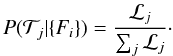 (14)The most likely type for
a given SN candidate is the one with the highest .
We co-add the probabilities for the subtypes belonging to either of the two main types
(thermonuclear and core collapse types) and obtain the probabilities
P(TN) and P(CC) for
each typed supernovae. Our tests of the typing using simulated data of the same quality
and type (see Sect. 4.1) indicate that the resulting
subtype classifications within these two main types are prone to quite large errors (in
the order of 10−20%), while the errors on the main type classifications are
significantly smaller (in the order of 5−10%).
(14)The most likely type for
a given SN candidate is the one with the highest .
We co-add the probabilities for the subtypes belonging to either of the two main types
(thermonuclear and core collapse types) and obtain the probabilities
P(TN) and P(CC) for
each typed supernovae. Our tests of the typing using simulated data of the same quality
and type (see Sect. 4.1) indicate that the resulting
subtype classifications within these two main types are prone to quite large errors (in
the order of 10−20%), while the errors on the main type classifications are
significantly smaller (in the order of 5−10%).
In Sect. 4 we discuss how to set constraints on the evidence and normalised probability to reliably reject both mis-classified and non-supernova objects.
We also constructed a “best-fit” light-curve for each supernova. This was made by fixing the supernova type and then finding the most likely value for each parameter one at a time, by marginalising over the remaining three parameters. As noted by Kuznetsova & Connolly (2007), Bayesian techniques do not always give the best estimate for the individual fitted parameters. To obtain trustworthy estimates of individual parameters, dedicated simulations have to be run, which is beyond the scope of this paper. We merely used the fitted light curves as a measure of the overall quality of fit (a method that is studied extensively by Monte-Carlo-simulated light curves, see Sect. 4.1).
3.3. Supernova subtype templates
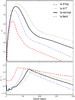 |
Fig. 1 Template light curves for the four thermonuclear supernova types at z = 0.5. The upper panel shows the R light curve for the Ia-normal subtype as solid (black), the Ia-faint subtype as dash-dotted (blue), the 91T-like subtype as dotted (green) and the 91bg-like subtype as dashed (cyan). In the lower panel the R−I colour evolution for the four subtypes is shown using the same line styles (this figure is available in colour in the electronic version of the article). |
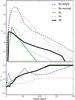 |
Fig. 2 Template light curves for the five core-collapse supernova types at z = 0.5. The upper panel shows the R light curve for the IIP subtype as thick solid (black), the IIn subtype as dash-dotted (red), the IIL subtype as solid (green), the Ibc-normal subtype as dotted (black) and the Ibc-bright subtype as dashed (blue). In the lower panel the R − I colour evolution for the five subtypes are shown using the same line styles (this figure is available in colour in the electronic version of the article). |
We used supernova spectra and absolute magnitude light curves to construct light curve templates for nine different supernova subtypes. The spectra and MB light curves for all these types were (with a few exceptions) obtained from Nugent (2007). The spectra we used extend from 1000 Å to 25 000 Å and cover epochs from day ~1−2 to ~100 after explosion. The light curves were scaled to the absolute peak magnitudes given in Table 2 and were obtained from Dahlen et al. (2004b and references therein) unless otherwise noted. The table contains a complete list of the references used in the construction of each template.
The output light curve template library consists of observer-frame light curves for the redshift range 0.01–2.0 (with a step size of 0.01 in z) in the VIMOS R and I filters for each of the nine supernova subtypes. As an example, Figs. 1 and 2 show the R band light curve and the R − I colour evolution for the nine templates at z = 0.5 (roughly corresponding to rest frame B and B − V). It should be noted that the similarities in colour between the Ibc-bright and Ibc-normal templates and for the IIP and IIL templates, respectively, arise because of the spectral templates used (see relevant sections below).
The subtype fractions listed in Table 2 are based on the measurements of Li et al. (2011b) and the compilation by Dahlen et al. (2004b) and were calculated for our magnitude limited sample using the limiting magnitudes from the light curve rejection step. These fractions were not used in the actual typing, but were only used to study the misclassification ratios, see Sect. 4.3.
3.3.1. Type Ia supernovae
We used four different light curve templates for the thermonuclear supernovae. The four templates (91bg-like, Ia-faint, Ia-normal, 91T-like, from fainter to brighter) have different absolute peak magnitudes and consequently different decline rates as well. The decline rates were parameterised using the stretch parameter, s, first introduced by Perlmutter et al. (1997). The range in stretch (s = 0.49–1.04) for the four templates provides a sparsely sampled grid that covers the observed stretch distribution of type Ia supernovae (e.g., Sullivan et al. 2006).
The spectra and rest-frame B light curve used to construct the Ia-normal and Ia-faint templates were first presented in Nugent et al. (2002). The absolute peak B magnitude used for the Ia-normal template, −19.34, was obtained from Tonry et al. (2003). The peak magnitude for the Ia-faint subtype was calculated by starting from the Ia-normal peak magnitude and scaling to a s = 0.8 peak magnitude using the luminosity-to-decline rate relationship from Phillips et al. (1999) and the decline-rate-to-stretch relation from Jha et al. (2006). The resulting absolute peak B magnitude is −18.96.
The light curve and spectra for the 91T–like template were first presented in Stern et al. (2004). These input data were corrected for extinction assuming {RV,E(B − V)} = {3.1/0.2} (Nugent 2007). The 91bg-like template is based on light curves and spectra of SN 1991bg and SN 1999by (Nugent et al. 2002). The peak absolute B magnitudes are, respectively, −19.64 and −17.84 (Tonry et al. 2003). The templates have stretch values according to their namesakes, 1.04 for the 91T-like template and 0.49 for the 91bg-like template.
3.3.2. Type Ib/c supernovae
We used two Ib/c supernova templates, the Ibc-bright and Ibc-normal templates. The spectral evolution is based on the work of Levan et al. (2005) and the light curve is based on observations of SN 1999ex from Hamuy et al. (2002). The observed data were corrected for extinction because the used SN have notable extinction, {RV,E(B − V)} = {3.1,0.4} is assumed (Nugent 2007). Richardson et al. (2006) find that the absolute peak magnitude distribution of Ib/c SNe can be described by using one bright and one normal population. We used the mean absolute peak magnitudes, −19.34 and −17.03, and scatter for the two populations from their paper; converting the magnitudes to our chosen cosmology and k-correcting to the B band. The data available in the SVISS do not allow a refinement of the Ibc typing into Ib and Ic subtypes, and it is not clear-cut that these two spectral types correspond to the two different photometric types (the bright and normal) considered in this work (Hamuy et al. 2002; Li et al. 2011b).
It should be noted that the red colour of the template in pre-peak epochs (the first 5−7 days in rest-frame) is the result of basing the template on SN 1999ex, which showed this effect at early epochs (Hamuy et al. 2002). There are not many Ib/c supernovae that have been observed before peak brightness, but observations of other Ib/c’s (e.g., SN 2008D from Modjaz et al. 2009) show that this effect may not be characteristic of the type. We performed tests using the typing code with a Ib/c template without the early red phase and found that the choice of template has very little influence on the resulting probabilities (less than 1%).
3.3.3. Type IIL supernovae
The IIL spectra and light curves were first used in Gilliland et al. (1999). The light curve is originally from Cappellaro et al. (1997). Richardson et al. (2002) presented the absolute B peak magnitude distribution of IIL SNe, and we adopt the mean peak magnitude and scatter for their normal IIL population. Converting the magnitude to our cosmology, we arrive at a B peak magnitude of −17.23.
3.3.4. Type IIn supernovae
The spectra and light curves are based on SN 1999el (Di Carlo et al. 2002), whereas the absolute B peak magnitude and scatter are obtained from Richardson et al. (2002). After compensating for the different cosmological parameters, the resulting peak magnitude is −18.82.
3.3.5. Type IIP supernovae
The spectra used to build the IIP supernova template come from different sources. For the early epochs (≤33 days after explosion) we used extinction-corrected spectral models from Dessart et al. (2008), which in turn are based on SWIFT UV-optical observations of SN 2005cs and SN 2006bp (Pastorello et al. 2006; Brown et al. 2007; Immler et al. 2007; Quimby et al. 2007). The late epoch spectra are based on SN 1999em from Baron et al. (2004) and obtained from Nugent (2007). The reason for not using the SN 1999em spectra for the early epochs is that the UV part of those spectra are modelled and extrapolated from optical observations, the more recent modelling based on early epoch UV/optical observations should therefore provide a more accurate spectral evolution.
The light curves were constructed using photometric data for SNe 1999em, 1999gi, 2003gd, 2004et, 2005cs and 2006bp (Elmhamdi et al. 2003; Leonard et al. 2002; Hendry et al. 2005; Sahu et al. 2006; Pastorello et al. 2006; Quimby et al. 2007). The light curve of each of these SNe was scaled to a common peak magnitude and corrected for extinction using the values given in the original references. Each curve was then re-sampled with a resolution of one day over the range of observed epochs (using spline interpolation). The final IIP light curve was then obtained by averaging over the six interpolated light curves. The adopted absolute B peak magnitude, −16.66, and scatter come from Richardson et al. (2002), again compensating for the cosmological parameter difference.
3.3.6. K-corrections of SN light curve templates
We then calculate VIMOS R and I apparent light curves
for the redshift range [0,2] using the following formula (similar
to Dahlen et al. 2004b): 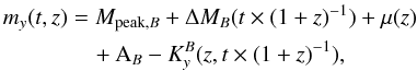 (15)where
y refers to the observed filter (R or
I), t is the observer frame epoch,
Mpeak,B is the peak absolute magnitude in
a rest-frame B filter, ΔMB
is the light curve decline relative to the peak, μ(z)
is the distance modulus and AB is the rest frame extinction
in the host galaxy. The K-correction
(15)where
y refers to the observed filter (R or
I), t is the observer frame epoch,
Mpeak,B is the peak absolute magnitude in
a rest-frame B filter, ΔMB
is the light curve decline relative to the peak, μ(z)
is the distance modulus and AB is the rest frame extinction
in the host galaxy. The K-correction  , following
the formalism of Kim et al. (1996), is given by
, following
the formalism of Kim et al. (1996), is given by
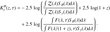 (16)In
this expression
(16)In
this expression  is the spectral energy distribution of Vega;
SB(λ),
Sy(λ) the Johnson
B and VIMOS R/I total filter
transmission curves and F(λ,τ) the spectral energy
distribution of the supernova at rest frame epoch τ.
is the spectral energy distribution of Vega;
SB(λ),
Sy(λ) the Johnson
B and VIMOS R/I total filter
transmission curves and F(λ,τ) the spectral energy
distribution of the supernova at rest frame epoch τ.
4. Testing the typing method
4.1. Simulated supernova light curves
To test the typing accuracy of the code applied to the observed SNe, we created a simulated mock detection catalogue. This catalogue was created to resemble the expected characteristics of the detected SN sample when it comes to peak magnitude distributions, light curve shapes, redshift distribution, and dust extinction. The catalogue also reflects the specifics of the SN search, including the cadence between observing epochs and the limiting magnitudes in the detection filters.
We first assumed a total SN rate by summing the thermonuclear (TN) and core-collapse (CC) rates from Dahlen et al. (2004b). We used this rate to assign a random redshift to each mock SN in the range 0 < z < 2. The SNe were thereafter given a main type, either TN or CC, from the relative strength of the rate of these types at the assigned redshift. The thermonuclear SNe were then subdivided into a faint, a normal, a 91bg-like and a 91t-like population, while the CC SNe were subdivided into IIL, IIP, IIn, Ibc-bright or Ibc-normal. It should be noted that the fractions of each simulated subtype are equal at this point. We did this to ensure that the number of simulated SNe for each subtype is sufficiently high for statistics, even for the rare subtypes. The fractions given for each subtype in Table 2 were used when analysing the typing results for the simulated light curves (see Sect. 4.3).
A peak B-band magnitude was assigned to each SN (Table 2). This was then perturbed using the peak magnitude dispersion values given in the table. Each SN was assigned an explosion date over the course of one year. We then used the actual cadence of the SN search and the B-band light curves for each specific type to calculate the absolute magnitude of the SN at the different observational epochs. Because the SN explosion dates are distributed over time, we will have some SNe that are observable in all epochs (i.e., those exploded before the first observation), and others that explode during the observational period and thus only observable in some of the epochs.
In the next step we used the type specific SEDs of the SNe to calculate the K-corrections that give us the apparent magnitudes in the observed R and I filters corresponding to the absolute B-band magnitudes (see Sect. 3.3.6). The apparent magnitudes were also corrected for extinction in the SN host galaxies using the extinction distributions from Riello & Patat (2005). In the final step, we added a photometric error to the apparent magnitudes. This consists of both a statistical part, derived from the expected S/N = 3 limits in R and I (see Sect. 2.3.2, and a “systematic” part, for which we assumed an extra 4% error in the flux. The simulated catalogue consists of apparent magnitudes and errors in R and I at each observational epoch. We treated objects with S/N < 1 as non-detections. This is also the case for epochs observed prior to the explosion of a particular SN.
Because we rely on photometric redshifts, we also assigned a simulated redshift to each SN, zsim. We calculated this by adding a random scatter, Δzrnd – drawn from a Gaussian distribution with σz = 0.06 – to the true redshift (ztrue) according to zsim = ztrue + (1 + ztrue) ∗ Δzrnd. The σz used here is the photometric redshift accuracy of our host galaxy catalogue, see Sect. 2.4.
When testing our code using the mock catalogue, we culled the sample by applying additional selection criteria. As our default set-up, we only included objects with a S/N > 3 in at least two consecutive epochs in both R and I (mimicking the set-up used for the observed supernovae). The total number of remaining simulated supernovae after the cull is ~18 000, which corresponds to roughly 2000 SNe per subtype (see Table 3).
Simulation results.
4.2. Rejection of non-supernovae
As mentioned in Sect. 3.2, the Bayesian typing
method only gives valid results when the input light curve can be modelled by one of the
templates. If the variability of a source has a non-SN origin (or, though less likely, is
a SN with a very irregular light curve), the resulting likelihoods will be very small.
Indeed, the evidence will be zero (within machine accuracy) in many cases where the
observed light curve is just too different from a template SN light curve. The evidence,
 (see Eq. (13)), can therefore be used to
reject possible anomalous sources (AGN, variable stars, complicated subtraction
residuals). We followed the suggestion of Kuznetsova
& Connolly (2007) and defined rejection limits for each template,
(see Eq. (13)), can therefore be used to
reject possible anomalous sources (AGN, variable stars, complicated subtraction
residuals). We followed the suggestion of Kuznetsova
& Connolly (2007) and defined rejection limits for each template,
 .
These were calculated by finding the evidence below which fall 99.9% of the evidences –
resulting from fitting of the Monte-Carlo-simulated light curves. The likelihood
thresholds are in the order of 10-100.
.
These were calculated by finding the evidence below which fall 99.9% of the evidences –
resulting from fitting of the Monte-Carlo-simulated light curves. The likelihood
thresholds are in the order of 10-100.
It should be noted that the likelihood threshold is only really efficient in removing sources with light curves that are sufficiently different from a supernova light curve. For example, an active galactic nuclei (AGN) with a light curve very similar to a supernova will of course not be removed by this cut. Using this rejection scheme allows us to perform an automatic cut that will only reject extreme outliers (0.1%) in the supernova population. Additional manual inspection is needed to safeguard against possible spurious candidates that have light curves similar enough to SNe to end up with likelihoods higher than the 99.9% threshold. This process is described, along with our final supernova candidates, in Sect. 5.
Some of the problems related to supernovae with non-standard light curves may be avoided by using the technique of “fuzzy” templates, pioneered by Rodney & Tonry (2009). This method enables the templates to cover more of the parameter space by giving the templates themselves an uncertainty (“fuzziness”). In this work we did not use this technique but it can be implemented into our code, and we will include it as an option in future versions of it. Another way to improve typing of these SNe is to use a more extended set of templates and to update the existing ones.
4.3. Systematic and statistical errors of typing
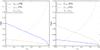 |
Fig. 3 Effect on the misclassification ratios of applying a rejection criterion on the type probability. The left/right panel shows the weighted misclassification ratios (floss,w and fgain,w) for the thermonuclear/core-collapse SNe along with the fraction of rejected candidates (Nrej/Napp) for a given limiting type probability (Plim). This information can be used to select an optimal Plim to avoid misclassifications without rejecting too many candidates. For details see the text and Table 3 (this figure is available in colour in the electronic version of the article). |
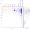 |
Fig. 4 Main panel: fit quality as measured by the absolute Bayesian likelihood for the best-fitting template (ℒmax), versus P, the probability of a given source being of the simulated type, for the ~18 000 Monte-Carlo-simulated supernovae. The upper panel shows the P distribution and the right panel the ℒmax distribution. For clarity, large (blue) dots and solid (blue) lines marks the correctly typed SNe (with P > 0.5); small (red) dots and dashed (red) lines the incorrectly typed SNe. The cross and star symbols in the main panel show ℒmax and P(TN)/P(CC), respectively, for the observed supernovae (see Sect. 5). Three of the thermonuclear SN candidates have ℒmax < 1 × 10-14, they are marked by a caret lower limit symbol at ℒmax < 1 × 10-14 (note that they have the same P(TN) values, thus the symbols are overlapping) (this figure is available in colour in the electronic version of the article). |
We used the Monte-Carlo-simulated supernova light curves to find the expected misclassification ratios for the two main supernova types at different redshifts. Typing of the simulated light curves was performed using the same code and assumptions as when typing the observed supernovae. This approach allows us to estimate the total errors on the supernova counts including both systematic errors, which arise from the assumed priors and possible systematic errors in the photometry; and statistical errors from the photometric statistical errors and the photometric redshift errors.
We investigated the errors by studying the misclassification ratios,
floss and fgain for the
simulated thermonuclear and core-collapse supernova light curves. The ratios are defined
as 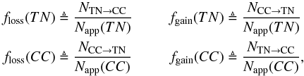 (17)where
NTN → CC and NCC → TN is the
number of SNe that were incorrectly classified (the true type on the left) and
Napp is the apparent number of SNe of the given type. For
example, floss(TN) gives the fraction of
thermonuclear SNe incorrectly classified as CC SNe. Note that using the ratios as measures
of misclassification errors is valid if the underlying core-collapse to thermonuclear SN
ratio in the survey is the same as the one we assume in Sect. 4.1.
(17)where
NTN → CC and NCC → TN is the
number of SNe that were incorrectly classified (the true type on the left) and
Napp is the apparent number of SNe of the given type. For
example, floss(TN) gives the fraction of
thermonuclear SNe incorrectly classified as CC SNe. Note that using the ratios as measures
of misclassification errors is valid if the underlying core-collapse to thermonuclear SN
ratio in the survey is the same as the one we assume in Sect. 4.1.
The different subtypes have quite different misclassification ratios. Because we assumed the SN frequency for the different subtypes to be equal, we also computed weighted misclassification ratios, floss,w(TN), fgain,w(TN), floss,w(CC), fgain,w(CC), where the number of misclassifications per subtype (e.g. NIIP → TN) are weighted by the relative frequency of that subtype. The subtype fractions are given in Table 2. The floss,w and fgain,w ratios were adopted as the final measure of misclassification errors in our survey.
Figure 3 shows how fgain,w(TN/CC) and floss,w(TN/CC) decrease when a limit on the type probabilities, Plim, for a source to be included in the analysis is introduced. The figure also shows that the use of a limiting probability will decrease the survey efficiency. Owing to the low-number statistics nature of our survey we elected not to use a limiting probability as a rejection criteria, but it should be noted that the misclassification errors can be somewhat decreased by only including objects with high probabilities. The ratios and total number of simulated supernovae for the different redshift bins can also be found in Table 3.
There is a caveat with using the misclassification results from the simulated sample. The errors are only really reliable when the observed supernova sample has light curves that are similar to the template light curves on average. If most of the observed supernovae have light curves different from the templates, the errors estimated by this method will not be representative. Figure 4 shows the distribution of Bayesian evidence for most likely type, ℒ, for the simulated SN sample together with the observed supernovae (see Sect. 5). Comparing the distribution in ℒ of the simulated SNe to the observed ones indicate that the samples seems to be fairly different.
A K − S test applied to the two samples is not conclusive, we cannot rule out that the two populations are the same with significance (the K − S p-value is 0.11). Interpreting this result is not trivial, there is a number of assumptions that go into simulating the SNe (the choice of specific templates and basically all of the priors) that can make the distribution different from what you would expect for a real sample. It is certainly possible that a discovered SNe may have a light curve that is simply different from any of the templates we use, which will cause a mismatch like the one we see in the ℒ distributions. This is also discussed in Sect. 4.2, where we provide some suggestions on how to solve the problem.
The assumption that the the supernovae will be evenly distributed into the subtypes (see Sect. 4.1) will influence the ℒ distribution and cause it to be slightly different from the observed distribution. In this particular case we cannot use the a priori subtype fractions to weight the results (as used in Sect. 4.3) because the numbers of observed SNe in the different types are too low for subtype K–S calculations.
There is consequently no reason to expect that the the samples would be perfectly matched (giving p-values close to 1). Nevertheless, we cannot rule out that the resulting p-values indicate that the assumption of the simulated light curves are representative of the sample of real supernovae (at a significance level of 10%). Note that the efficient number of data points for the two types are quite low (~7 for the thermonuclear and ~9 for the core-collapse SNe, see Sect. 5). A better accuracy for the p-values requires more real supernovae to compare with, which would also enable us to look at the subtype statistics.
4.4. Redshift determination with the typing code
By fixing the type to the most likely template found in the full Bayesian fitting run, we tried to find the most likely redshift of the supernovae (see Sect. 3.2 for a more detailed description). The prior on redshift is based on the probability distribution for photometric redshift of the host galaxies. By looking at the most likely redshifts obtained from the typing of the simulated supernovae, we investigated whether the prior information added through the supernova light curve changes the redshift accuracy.
For the SVISS host galaxies the normalised photometric redshift scatter is σz = rms((ztrue − zobs)/(1 + ztrue)) = 0.06, the simulated SN redshifts are scattered according to this (see Sect. 4.1). When comparing the most likely redshifts (zfit) from the typing code with the true ones (ztrue as defined in Sect. 4.1), we found a normalised redshift scatter of 0.067 for the thermonuclear supernovae and 0.072 for the core-collapse with a negligible offset for both types. Overall, a small number of objects (<0.1%) were assigned a catastrophic redshift, defined as objects with (| zfit − ztrue|/(1 + ztrue) > 0.2; these are all misclassified SNe. The resulting redshift accuracy is thus very similar to the input simulated error, the inclusion of prior information in the form of the supernova data did not improve the redshift determination. On the other hand, excluding the misclassified supernovae, no additional errors to the redshift estimates seem to have been introduced in the typing code.
Supernovae in the SVISS.
In Table 3 we also present the redshift scatter for the simulated supernovae in the redshift bins used to study misclassification. Note that the scatter values in the table are not normalised (i.e. dz = stdev(ztrue − zobs))), as opposed the the σz discussed in the previous section. The overall redshift accuracy is consistent with the simulated input accuracy. The 0.25 < z ≤ 0.5 redshift bin has a somewhat increased scatter, this is because of a higher contribution of catastrophic redshifts (or, equivalently, misclassified SNe) in this bin. The actual percentage of outliers in this bin is still quite low, 3% for the thermonuclear and 4% for the core-collapse SNe.
4.5. SDSSII supernovae
We also tested our typing code on a small sample of spectroscopically confirmed supernovae from the SDSS supernova survey (Frieman et al. 2008). The sample contains 55 Ia supernovae at z = 0.001−0.2 and 32 IIP supernovae at z = 0.001−0.2 (Frieman et al. 2008; Kessler et al. 2009, 2010b; D’Andrea et al. 2010). The observations were obtained with a cadence (1−10 days) and total survey length (~90 days). To be able to compare the typing results from this sample with the observations and simulations for the SVISS, we re-sampled the SDSS supernova light curves to a cadence of ~20 days (yielding 4−5 epochs). The resulting light curves (at z ~ 0.1) therefore sample approximately the same rest-frame epochs as the light curves from SVISS (with a mean redshift of 0.57). We used the SDSS g and r filters, which at z ~ 0.1 target similar rest-frame colours as the VIMOS R and I filters at z ~ 0.5. Using only these epochs and filters will of course render the typing less optimal, but will render the results comparable to the SVISS typing because the same rest-frame light curve information is used. Note that a maximum of five epochs can be fitted using this sampling, compared to the maximum of seven used in the SVISS observations and simulations.
The results of testing performed on the sample of SDSS supernovae do not show any significant differences with the Monte-Carlo-simulated sample in terms of misclassification. The total misclassification percentage for a sample of 55 Ia supernovae (i.e., Ia supernovae typed as any of the core-collapse subtypes) is 7.3%. The total misclassification percentage for a sample of 32 IIP supernovae is 9.3%. These ratios are of the same order of magnitude as the results obtained for the simulated sample, although slightly higher. The simulated Ia SNe are misclassified in ~3% of the cases in the relevant redshift bin, the corresponding percentage for IIP SNe is ~5%. The difference could be caused by the somewhat lower number of data-points available, on average, for the SDSSII SNe with resampled light curves. We conclude that the simulations provide valid estimates on the misclassification ratios for a real sample of supernova light curves.
5. Results
After applying the photometric rejection criterion described in Sect. 2.3.2, we ended up with 115 supernova candidates that are typed using our
code. The subtype probabilities for the two main types are co-added, yielding
P(TN) and P(CC), for
each candidate; the candidate was assigned the main type with the highest probability.
ℒmax for the candidate is the maximum evidence among the subtypes belonging to
the chosen main type. The evidence was then compared to the threshold evidence,
(see Sect. 4.2), and candidates with lower
ℒmax than the threshold were rejected. The remaining number of candidates at
this point was 54, the rejected objects were also manually checked to ensure that the
technique was working.
We then investigated each of the 54 possible supernovae manually, making an overall assessment – using both the images, light curve and classification – of whether the source is likely a supernova or something else. This investigation was performed by six of us (JM, TD, GÖ, LMT, JS, and SM), and we individually and separately rated each candidate. The manual rejection step allows us to remove spurious transient sources from imperfect image subtraction. These residuals can be present in both bands and in multiple epochs, which enabled them to get through the earlier rejection steps. During the manual inspection of both images and light curves, the residuals can be discovered. The choice of having several independent inspectors minimises the risk of errors being made. The rejected residuals have a number of properties in common: they all have a bright host galaxy, in general they tend to move (by 0.1−1 pixels) from epoch to epoch, most of them have low ℒmax and have erratic light curves combined with large errors, most of them also show a negative residual close to the source in at least one epoch/filter. Approximately 20 candidates are considered to be spurious subtraction residuals. A small number of candidates (<5) is found very close to the edge of the images and are related to the the higher noise level at the edges. A reanalysis of the photometric errors in these regions showed that the sources did not fulfil our photometric criteria, we consequently decided to reject these sources. This decision also means that the efficient field of view will be somewhat smaller, a trade-off we are willing to accept to make the detection efficiency of the survey constant over the full field. After this rejection step we were left with 31 transient sources that we believe are real. The world coordinates, RI light curves and errors for the 31 transient sources are given in the appendix.
At this point we also rejected possible AGN that contaminate our sample. To do this we used subtracted frames with a two-year difference in time (the reference epoch from August 2003 and the control epoch obtained in November 2005 to January 2006). If a candidate showed variability over this time span, it is very unlikely to be a supernova, and we rejected it (with the exception of one candidate, discussed in Sect. 5.2). Of the 31 candidates 15 were rejected because of this, but note that some of these are likely not AGN but rather some other non-SN transient object (at least one of them has a light curve and colour consistent with a variable star). It should be noted that the AGN rejection scheme will not allow us to get rid of AGN that show no variation over the two-year baseline and have a SN-like light curve during the search period; however, the number of AGN fulfilling this criterion is estimated to be small (also see Sect. 5.3).
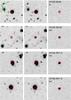 |
Fig. 5 R-band image cutouts, approximately 20 × 20″ large of the supernova candidates SVISS-SN43, SVISS-SN161, SVISS-SN115 and SVISS-SN116. The leftmost panels show the reference image, middle panels show the peak brightness (observed) epoch and the rightmost panels show the subtracted image at peak brightness. The (red) circle marks the location of the supernova as detected in the subtracted frame. The most likely redshifts (from the typing code) for these SNe are (starting at the top) 0.43, 0.50, 0.40 and 0.55, respectively. |
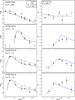 |
Fig. 9 Observed and fitted light curves for the supernova candidates SVISS-SN43, SVISS-SN161, SVISS-SN115, and SVISS-SN116. The left-hand panels show the observed R (solid hexagons) and I (squares) light curves along with the best-fit light curve of the most likely supernova subtype, solid (black) for R and dashed (blue) for I. The error bars given for the observations are based on the photometric accuracy simulations described in Sect. 2.3.2. If the source is non-detected (i.e., has an estimated magnitude error of more than 1), a magnitude lower limit is given. The right-hand panels show the R − I colour evolution. For the R − I plot, the limit symbols indicate that the source was only detected in one of the bands and a lower or upper limit is given (this figure is available in colour in the electronic version of the article). |
The final sample of 16 supernovae is presented in Table 4, cutout images for each SN are available in Figs. 5 through 8. Figures 9 through 12 show the observed and best-fit light curves for all of them. The best-fit light curves are here obtained as described in Sect. 3.2, it should be noted that the typing method is not based on finding the best-fitting (in the χ2 sense) parameter set but rather on finding the type with the closest matching parameter space given the priors. Nevertheless, the fitted light curves provide a quick estimate on how good the evidence for the most probable type is, a fitted light curve far from the observed curve usually also means that the evidence is low. The probability (P) might be close to one even for low ℒmax, this reflects that the chosen type might be improbable in the absolute sense but that the type is the best among the available alternatives.
The redshift distribution, based on the fitted redshifts from the typing, of the supernovae is shown in Fig. 13. The joint distribution (the filled bars in the plot) has a mean of 0.58. The thermonuclear supernovae are on average found at lower redshifts compared to those of the core-collapse (with a mean of 0.51 compared to 0.64). The requirement that the supernovae should be detected in both filters makes this expected because thermonuclear SNe become very faint at redshifts ≳0.8 in the R-band owing to k-corrections.
5.1. Thermonuclear supernovae
Seven of the 16 supernovae in the survey are found to have a thermonuclear origin. Based on the simulation results, approximately 0.7 (10% of the total number) could be misclassified core-collapse supernovae. Inspecting the light curves and looking at the fit quality (P(TN) and ℒbest) we can see that one of the seven supernovae (SVISS-SN43) has a somewhat insecure typing. The probability, P(TN), is well below 1.0, which means that it has a significant chance of being a core-collapse supernova.
Three of the supernovae (SVISS-SN161, SVISS-SN115, and SVISS-SN309) have low evidences (ℒbest). They all have probabilities close to 1.0, however, indicating that they, while not being perfectly matched by the available templates and priors, are optimally fit by the thermonuclear templates. The addition of a more general stretch prior as described in Sect. 3 would most probably allow the templates to match the observed light curves better.
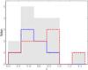 |
Fig. 13 Redshift distribution of the supernovae detected in the SVISS ELAIS-S1 field using a z bin size of 0.25. The redshifts used are the resulting best-fit redshifts from the supernova typing code. The grey, filled bars show the total supernova counts, the blue (dotted) lines show the distribution of thermonuclear SNe and the red (dashed) lines the distribution of core-collapse SNe (this figure is available in colour in the electronic version of the article). |
5.2. Core-collapse supernovae
Nine of the supernovae are found to be best matched by a core-collapse template light curve. The simulation results indicate that none of these are likely to be misclassified thermonuclear supernovae (2.4% of the total number). A look at the actual fit qualities for the supernovae show that three of them (SVISS-SN14, SVISS-SN261, and SVISS-SN24) have probability values lower than 0.8 and accordingly have a definite probability of being misclassified thermonuclear SNe. It is worth noting that for two of them the most likely subtype is Ibc, the CC subtypes with light curves most similar to the thermonuclear subtypes. They are also all quite faint and detected only in 2−3 epochs. However, we have no reason to mistrust the likelihoods computed for these SNe and thus conclude that they are likely of core-collapse origin.
One of the CC supernovae, SVISS-SN56, has a low evidence (also visible in the light curve fit, see Fig. 12), indicating that none of the supernova templates fitted the data well. Including more core-collapse supernova templates, improving the ones used or adding a colour prior could make it possible to get a better typing result for this supernova.
As discussed in Sect. 2.4, for three CC SNe no photometric redshift prior was used. In the case of SVISS-SN14 this is because the most likely redshift (0.36) for the found subtype, IIn, is significantly different from the photometric redshift of the host galaxy (0.76). This type and redshift is found to be the best fit even when the photometric redshift is used as a prior. The reason for this mismatch could be either that the host redshift is incorrect (approximately 10% of the photometric redshifts are so called catastrophic redshifts, off by more than 0.3, again see Sect. 2.4), or that there is another very faint and undetected galaxy that is the real host of the SN. A third possibility is that the supernova is of a peculiar type that is not well-modelled by the template light curves.
For SVISS-SN261, the closest galaxy is quite far away in angular distance and it has a redshift of 1.64. Using this as a redshift prior results in the SNe being placed at a redshift of 0.37 as a Ibc-bright subtype. There is just no possible SN type that can give the observed light curve at such a high redshift. Also, using a flat prior on the redshift results in the same type and redshift. We believe that the true host of this SN is undetected, it could possibly be a low-surface brightness, but star-forming galaxy at intermediate redshift.
The third of the three “hostless” SNe is a complicated case. SVISS-SN31 is located very close to a very faint galaxy with a photometric redshift of 2.97. At that redshift all of the supernova types under consideration would be undetectable (owing to distance dimming and k-corrections). Using a flat prior on the redshift results in a type IIL SN at z = 0.12. Other nearby galaxies (in angular distance) have been considered as hosts, but none of them has a redshift lower than ~0.6. The second-closest galaxy has a photometric redshift of 1.04 (highly uncertain, the 68% confidence interval for this measurement is 0.96–1.58), and if this is used as a prior for the supernova typing the resulting type is a IIn SN at z = 1.92. However, the evidence for this type is lower than the IIL solution found with a flat prior. Redshift priors from the other nearby galaxies result in even worse evidence for the most likely types. It should also be noted that the main type (CC) of the supernova is the same for all the tested redshift priors. Based on the evidence comparisons, host galaxy properties, and angular distance we conclude that the typing without a redshift prior provides the most believable solution. The mismatch with the host redshift could be explained by, as for SVISS-SN14 above, the host galaxy redshift being catastrophically wrong, a faint undetected host galaxy, or a peculiar SN type.
5.3. A peculiar SN candidate
In Sect. 5 we described how the AGN that likely contaminate the sample are dealt with. One of the variable sources showing variability over a two year period, SVISS-T167 has an intriguing light curve that could possibly come from a supernova with a very extended light curve. However, the supernova would in that case have to be of a peculiar type; our typing code was unable to find the most likely type (i.e. ℒbest < ℒ99.9, as defined in Sect. 4.2). The light curve of this candidate is shown in Fig. 14 and an image cutout is shown in Fig. 15. For it to be even remotely similar to a normal supernova light curve, it needs to be situated at high redshift where cosmological time dilation will stretch the light curve by a factor of 2 (or more).
Comparing this to the light curves of bright peculiar supernovae we find that the light curve is marginally consistent with that of a pair instability (PI) supernovae at high redshift, something that has also been suggested by Gal-Yam et al. (2009) for SN 2007bi and by Woosley et al. (2007) for SN 2006gy. PI SNe have slowly evolving light curves, sometimes with a secondary peak; the slow light curve decline of our candidate indicates that it could be similar to such SNe. The PI light curve in Fig. 14 was derived by taking a model rest frame B band light curves for a 110 M⊙ progenitor from the supplemental information available for Woosley et al. (2007) and shifting it to z = 1.0, applying time dilation and distance modulus. We did not attempt any detailed k-correction, but it should be noted that the correction term should be fairly small because the rest frame B central wavelength at z = 1.0 is close to the central wavelength of the I filter. We also compared the light curve to that of SN 2010gx (Pastorello et al. 2010), an extremely luminous type Ic-like supernova. We found that the very extended light curve and colour evolution of our transient is impossible to match with the 2010gx light curve, even when shifting it to higher redshift.
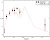 |
Fig. 14 I-band light curve of SVISS-T167. Also shown is a B-band light curve for a pair instability SNe shifted to z = 1 (line). Details of how the comparison light curve is constructed can be found in the text (this figure is available in colour in the electronic version of the article). |
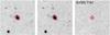 |
Fig. 15 I-band image cutouts, approximately 20 × 20″ large of the transient of unknown type, SVISS-T167. The leftmost panel shows the reference image, middle panel shows the peak brightness (observed) epoch and the rightmost panel shows the subtracted image at peak brightness. The (red) circle marks the location of the transient as detected in the subtracted frame. |
There is no strong evidence for our candidate being a supernova of this type, it is still a distinct possibility that the source is actually an AGN because the position of the source is right in the centre of its host galaxy. The photometric redshift for the host galaxy is not constrained, which might point towards it being an AGN (our photometric redshift code does not include AGN SED templates), but could also mean that it is a high-redshift galaxy (z ≳ 1) where the lack of near infrared data renders the photometric redshift technique unreliable. We excluded the source from the SN sample presented in Table 4. To discover the true identity of the object, follow-up observations of its host galaxy are needed.
6. Summary and discussion
We have presented light curves and typing of the 16 supernovae discovered by SVISS. Using photometric redshifts estimated from host galaxy photometry, we typed the SNe into thermonuclear or core-collapse events. The typing uses spectral and light curve templates for nine different subtypes and is based on a Bayesian fitting method. From studying Monte-Carlo-simulated SN light curves and a small sample of SDSS SN light curves, we conclude that the typing code yields reliable results considering that we only have photometric redshifts with accuracies in the order of 0.1, only one colour, and a limited number of epochs. We find that probably not more than 5–10% of the supernovae are misclassified. The misclassification ratios are not symmetric with respect to the two main types, a CC SN is more likely to be misclassified into a TN SN than the other way around.
Comparing our typing quality with that of other typing codes is not straight-forward because the input data and tests of the codes vary considerably. Kessler et al. (2010a) try to remedy this by offering a test sample of SN light curves and a framework in which different typing codes can be compared. Currently, our code is written specifically to deal with the data from SVISS, trying the code out on the test sample is thus outside the scope of this paper. Nevertheless, we can compare the typing quality estimated from our Monte-Carlo-simulated light curves with the typing qualities reported in Kessler et al. (2010a). The Ia efficiency, which in our paper is equal to (Napp(TN) − NTN → CC)/Ntot(TN), and Ia pureness, (Napp(TN) − NTN → CC)/(Napp(TN) − NTN → CC + NCC → TN) in our notation, are two of the concepts used to describe the quality in Kessler et al. (2010a). Our overall efficiency and pureness values for the thermonuclear SNe, 0.97 and 0.75, respectively, are comparable to the results obtained by the other typing codes, but with the caveat that we did not use the same test sample of supernovae as these authors.
Out of the 16 SNe,  are
core-collapse supernovae, and
are
core-collapse supernovae, and  are
thermonuclear; only the systematic typing errors derived from the misclassification ratios
are given here. The mean redshift for the entire sample is 0.58 with the core-collapse SNe
being at slightly higher redshifts than the thermonuclear ones. In a supernova survey of
this type a large number of spurious sources will be detected and methods must be devised to
safely reject interlopers without compromising the SN detection efficiency. We used a
combination of automatic (SExtractor, signal-to-noise rejection, SN typing rejection) and
manual (by-eye inspection of image frames by multiple independent observers, by-eye
inspection of light curves by multiple independent observers) rejection methods to ensure
that the final SN sample is as pure as possible.
are
thermonuclear; only the systematic typing errors derived from the misclassification ratios
are given here. The mean redshift for the entire sample is 0.58 with the core-collapse SNe
being at slightly higher redshifts than the thermonuclear ones. In a supernova survey of
this type a large number of spurious sources will be detected and methods must be devised to
safely reject interlopers without compromising the SN detection efficiency. We used a
combination of automatic (SExtractor, signal-to-noise rejection, SN typing rejection) and
manual (by-eye inspection of image frames by multiple independent observers, by-eye
inspection of light curves by multiple independent observers) rejection methods to ensure
that the final SN sample is as pure as possible.
In the specific case of AGN interlopers we find that the use of an additional observing epoch displaced from the search/reference epochs by at least one year makes it possible to limit the amount of contamination further. We also find that most of the AGN will also be rejected in the supernova typing step, because the fitting code is simply not able to fit the SN templates to their colour and evolution. At least one of the rejected candidates could possibly be a supernova of an extremely rare type. This particular source was still detectable, albeit barely, one year after our search period ended. The extremely extended light curve is comparable to that of pair instability SNe (Woosley et al. 2007) at high redshifts.
The SVISS results show that SN imaging searches combined with photometric typing can be used to find and characterise SNe at high redshifts. While the basic strategy used in this project does work, there are a few improvements that could be considered. One of the main uncertainties in the SN typing is the use of photometric redshifts. Securing more precise redshifts for the host galaxies would make the typing considerably more accurate. These redshifts could be in the form of well-calibrated photometric or spectroscopic redshifts. Future pencil beam surveys targeting high-redshift SNe should thus be aimed at regions with good spectral and multiwavelength coverage. We found the cadence of the search to be more or less optimal, given the constraint on total observational time, but with more frequent observations it should be possible to detect the UV breakout phase of core collapse SNe as well (e.g., Tominaga et al. 2011). Observations in more than one filter is mandatory to be able to do photometric typing, but we also found it to be quite important for rejecting spurious objects in the detection step. Adding more filters will break some of the degeneracies in the typing, but the typing accuracy is also limited by the quality of the templates.
A full analysis of supernova and star-formation rates based on our observations will be presented in a forthcoming paper (Melinder et al., in prep.). The work presented in this paper will help us estimate the uncertainties of the found rates. To calculate proper rates, information about the detection efficiency and the enforced photometric limits has to be taken into account. Nevertheless, a quick look at the raw numbers of discovered SNe of the two types compared to Monte-Carlo-simulations of detectable SNe using supernova rates based on local observations and star-formation rates (Dahlén & Fransson 1999) shows that our numbers are consistent with the expected rates. We can also compare the range and distribution in redshift of our supernovae to that of other surveys. Our sample of thermonuclear SNe are not really unique in this respect (see, e.g., Neill et al. 2006; Poznanski et al. 2007b; Dahlen et al. 2008), but it should be noted that the survey methodology we used is different from most other surveys where the requirement of spectra means that some of the fainter events may be missed. For the core-collapse SNe our sample is similar to the observations presented in Dahlen et al. (2004b) with 17 CC SNe at z < 0.7. We detect 9 CC SNe out to z = 1.4, with most of them at z ~ 0.8, and this is therefore one of the deepest survey to date for CC SNe.
Online material
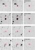 |
Fig. 6 R-band image cutouts for the supernova candidates SVISS-SN309, SVISS-SN402, SVISS-SN135 and SVISS-SN14. See Fig. 5 for descriptions on the different panels and marks. The most likely redshifts (from the typing code) for these SNe are (starting at the top) 0.47, 0.22, 0.98 and 0.36, respectively. |
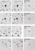 |
Fig. 7 R-band image cutouts for the supernova candidates SVISS-SN51, SVISS-SN54, SVISS-SN261 and SVISS-SN55. See Fig. 5 for descriptions on the different panels and marks. The most likely redshifts (from the typing code) for these SNe are (starting at the top) 0.51, 0.77, 0.37 and 0.83, respectively. |
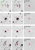 |
Fig. 8 R-band image cutouts for the supernova candidates SVISS-SN31, SVISS-SN56, SVISS-SN357 and SVISS-SN24. See Fig. 5 for descriptions on the different panels and marks. The most likely redshifts (from the typing code) for these SNe are (starting at the top) 0.12, 0.57, 1.4 and 0.81, respectively. Note that the host galaxy for SN357 is blended with a foreground galaxy, the selected host is the lowermost of the two galaxies. |
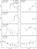 |
Fig. 10 Observed and fitted light curves for the supernova candidates SVISS-SN309, SVISS-SN402, SVISS-SN135, and SVISS-SN14. See Fig. 9 for descriptions on the different panels and marks. |
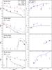 |
Fig. 11 Observed and fitted light curves for the supernova candidates SVISS-SN51, SVISS-SN54, SVISS-SN261, and SVISS-SN55. See Fig. 5 for descriptions on the different panels and marks. |
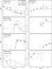 |
Fig. 12 Observed and fitted light curves for the supernova candidates SVISS-SN31, SVISS-SN56, SVISS-SN357, and SVISS-SN24. See Fig. 5 for descriptions on the different panels and marks. |
Appendix A: Observational data for the 31 transient objects
This appendix contains a table with extended information for the 31 transient objects detected in the SVISS ELAIS-S1 field. The astrometry is accurate to within 0.4″ (for details on the astrometry see Mencía-Trinchant et al., in prep.). The photometrical errors are obtained as described in Sect. 2.3.2. For non-detections the magnitude is given as a lower limit and the limit is also given as the error. The limiting magnitudes given in the table are 1σ limiting magnitudes derived from the photometric accuracy investigation. The host galaxy redshifts given in the table are photometric redshifts derived from the UBVRI galaxy photometry. Objects that were assumed to be hostless are given a redshift of N/A in the table.
Extended information on the transient objects.
Acknowledgments
We thank A. Pastorello for comments on the peculiar SN candidate and the SDSS supernova team for the use of the unpublished SN Ia data. We also thank A. Jerkstrand for helpful discussions regarding parallelisation of the typing code. We thank the anonymous referee for some helpful comments that helped us improve the paper. The observations were made in service mode at the VLT/VIMOS instrument at Paranal Observatories. We are grateful for financial support from the Swedish Research Council. S.M. and J.M. acknowledge financial support from the Academy of Finland (project:8120503).
References
- Alard, C. 2000, A&AS, 144, 363, (A00) [NASA ADS] [CrossRef] [EDP Sciences] [Google Scholar]
- Alard, C., & Lupton, R. H. 1998, ApJ, 503, 325 [NASA ADS] [CrossRef] [Google Scholar]
- Amanullah, R., Lidman, C., Rubin, D., et al. 2010, ApJ, 716, 712 [NASA ADS] [CrossRef] [Google Scholar]
- Astier, P., Guy, J., Regnault, N., et al. 2006, A&A, 447, 31 [NASA ADS] [CrossRef] [EDP Sciences] [Google Scholar]
- Barbary, K., Aldering, G., Amanullah, R., et al. 2010 [arXiv:1010.5786] [Google Scholar]
- Baron, E., Nugent, P. E., Branch, D., & Hauschildt, P. H. 2004, ApJ, 616, L91 [NASA ADS] [CrossRef] [Google Scholar]
- Barris, B. J., & Tonry, J. L. 2004, ApJ, 613, L21 [NASA ADS] [CrossRef] [Google Scholar]
- Bazin, G., Palanque-Delabrouille, N., Rich, J., et al. 2009, A&A, 499, 653 [NASA ADS] [CrossRef] [EDP Sciences] [Google Scholar]
- Berta, S., Rubele, S., Franceschini, A., et al. 2008, A&A, 488, 533 [NASA ADS] [CrossRef] [EDP Sciences] [Google Scholar]
- Bertin, E., & Arnouts, S. 1996, A&AS, 117, 393 [NASA ADS] [CrossRef] [EDP Sciences] [Google Scholar]
- Botticella, M. T., Riello, M., Cappellaro, E., et al. 2008, A&A, 479, 49 [NASA ADS] [CrossRef] [EDP Sciences] [Google Scholar]
- Brown, P. J., Dessart, L., Holland, S. T., et al. 2007, ApJ, 659, 1488 [NASA ADS] [CrossRef] [Google Scholar]
- Calzetti, D., Armus, L., Bohlin, R. C., et al. 2000, ApJ, 533, 682 [NASA ADS] [CrossRef] [Google Scholar]
- Cappellaro, E., Turatto, M., Tsvetkov, D. Y., et al. 1997, A&A, 322, 431 [NASA ADS] [Google Scholar]
- Cardelli, J. A., Clayton, G. C., & Mathis, J. S. 1989, ApJ, 345, 245 [NASA ADS] [CrossRef] [Google Scholar]
- Coleman, G. D., Wu, C., & Weedman, D. W. 1980, ApJS, 43, 393 [NASA ADS] [CrossRef] [Google Scholar]
- Dahlén, T., & Fransson, C. 1999, A&A, 350, 349 [NASA ADS] [Google Scholar]
- Dahlén, T., Fransson, C., Östlin, G., & Näslund, M. 2004a, MNRAS, 350, 253 [NASA ADS] [CrossRef] [Google Scholar]
- Dahlen, T., Strolger, L.-G., Riess, A. G., et al. 2004b, ApJ, 613, 189 [NASA ADS] [CrossRef] [Google Scholar]
- Dahlen, T., Strolger, L.-G., & Riess, A. G. 2008, ApJ, 681, 462 [NASA ADS] [CrossRef] [Google Scholar]
- Dahlen, T., Mobasher, B., Dickinson, M., et al. 2010, ApJ, 724, 425 [NASA ADS] [CrossRef] [Google Scholar]
- D’Andrea, C. B., Sako, M., Dilday, B., et al. 2010, ApJ, 708, 661 [NASA ADS] [CrossRef] [Google Scholar]
- Dessart, L., Blondin, S., Brown, P. J., et al. 2008, ApJ, 675, 644 [NASA ADS] [CrossRef] [Google Scholar]
- Di Carlo, E., Massi, F., Valentini, G., et al. 2002, ApJ, 573, 144 [NASA ADS] [CrossRef] [Google Scholar]
- Dilday, B., Smith, M., Bassett, B., et al. 2010, ApJ, 713, 1026 [NASA ADS] [CrossRef] [Google Scholar]
- Elmhamdi, A., Danziger, I. J., Chugai, N., et al. 2003, MNRAS, 338, 939 [NASA ADS] [CrossRef] [Google Scholar]
- Frieman, J. A., Bassett, B., Becker, A., et al. 2008, AJ, 135, 338 [Google Scholar]
- Gal-Yam, A., Mazzali, P., Ofek, E. O., et al. 2009, Nature, 462, 624 [NASA ADS] [CrossRef] [PubMed] [Google Scholar]
- Giacconi, R., Rosati, P., Tozzi, P., et al. 2001, ApJ, 551, 624 [NASA ADS] [CrossRef] [Google Scholar]
- Gilliland, R. L., Nugent, P. E., & Phillips, M. M. 1999, ApJ, 521, 30 [NASA ADS] [CrossRef] [Google Scholar]
- Glazebrook, K., Verma, A., Boyle, B., et al. 2006, AJ, 131, 2383 [NASA ADS] [CrossRef] [Google Scholar]
- Goobar, A. 2008, ApJ, 686, L103 [NASA ADS] [CrossRef] [Google Scholar]
- Hamuy, M., Maza, J., Pinto, P. A., et al. 2002, AJ, 124, 417 [NASA ADS] [CrossRef] [Google Scholar]
- Hendry, M. A., Smartt, S. J., Maund, J. R., et al. 2005, MNRAS, 359, 906 [NASA ADS] [CrossRef] [Google Scholar]
- Immler, S., Brown, P. J., Milne, P., et al. 2007, ApJ, 664, 435 [NASA ADS] [CrossRef] [Google Scholar]
- Jha, S., Kirshner, R. P., Challis, P., et al. 2006, AJ, 131, 527 [NASA ADS] [CrossRef] [Google Scholar]
- Johnson, B. D., & Crotts, A. P. S. 2006, AJ, 132, 756 [NASA ADS] [CrossRef] [Google Scholar]
- Kankare, E., Mattila, S., Ryder, S., et al. 2008, ApJ, 689, L97 [NASA ADS] [CrossRef] [Google Scholar]
- Kessler, R., Becker, A. C., Cinabro, D., et al. 2009, ApJS, 185, 32 [NASA ADS] [CrossRef] [Google Scholar]
- Kessler, R., Bassett, B., Belov, P., et al. 2010a, PASP, 122, 1415 [NASA ADS] [CrossRef] [Google Scholar]
- Kessler, R., Cinabro, D., Bassett, B., et al. 2010b, ApJ, 717, 40 [NASA ADS] [CrossRef] [Google Scholar]
- Kim, A., Goobar, A., & Perlmutter, S. 1996, PASP, 108, 190 [NASA ADS] [CrossRef] [Google Scholar]
- Kinney, A. L., Calzetti, D., Bohlin, R. C., et al. 1996, ApJ, 467, 38 [NASA ADS] [CrossRef] [Google Scholar]
- Kuznetsova, N. V., & Connolly, B. M. 2007, ApJ, 659, 530 [NASA ADS] [CrossRef] [Google Scholar]
- La Franca, F., Gruppioni, C., Matute, I., et al. 2004, AJ, 127, 3075 [NASA ADS] [CrossRef] [Google Scholar]
- LeFevre, O., Saisse, M., Mancini, D., et al. 2003, in Instrument Design and Performance for Optical/Infrared Ground-based Telescopes, ed. M. Iye, & A. F. M. Moorwood, SPIE Conf., 4841, 1670 [Google Scholar]
- Leonard, D. C., Filippenko, A. V., Li, W., et al. 2002, AJ, 124, 2490 [NASA ADS] [CrossRef] [Google Scholar]
- Levan, A., Nugent, P., Fruchter, A., et al. 2005, ApJ, 624, 880 [NASA ADS] [CrossRef] [Google Scholar]
- Li, W., Chornock, R., Leaman, J., et al. 2011a, MNRAS, 412, 1473 [NASA ADS] [CrossRef] [Google Scholar]
- Li, W., Leaman, J., Chornock, R., et al. 2011b, MNRAS, 412, 1441 [NASA ADS] [CrossRef] [Google Scholar]
- Magnelli, B., Elbaz, D., Chary, R. R., et al. 2009, A&A, 496, 57 [NASA ADS] [CrossRef] [EDP Sciences] [Google Scholar]
- Maoz, D., & Badenes, C. 2010, MNRAS, 407, 1314 [NASA ADS] [CrossRef] [Google Scholar]
- Mattila, S., Väisänen, P., Farrah, D., et al. 2007, ApJ, 659, L9 [NASA ADS] [CrossRef] [Google Scholar]
- Melinder, J., Mattila, S., Östlin, G., Mencía Trinchant, L., & Fransson, C. 2008, A&A, 490, 419 [NASA ADS] [CrossRef] [EDP Sciences] [Google Scholar]
- Miknaitis, G., Pignata, G., Rest, A., et al. 2007, ApJ, 666, 674 [NASA ADS] [CrossRef] [Google Scholar]
- Modjaz, M., Li, W., Butler, N., et al. 2009, ApJ, 702, 226 [NASA ADS] [CrossRef] [Google Scholar]
- Morokuma, T., Doi, M., Yasuda, N., et al. 2008, ApJ, 676, 163 [NASA ADS] [CrossRef] [Google Scholar]
- Neill, J. D., Sullivan, M., Balam, D., et al. 2006, AJ, 132, 1126 [NASA ADS] [CrossRef] [Google Scholar]
- Nugent, P. 2007, Peter Nugent’s Spectral Templates, http://supernova.lbl.gov/~nugent/nugent_templates.html [Google Scholar]
- Nugent, P., Kim, A., & Perlmutter, S. 2002, PASP, 114, 803 [NASA ADS] [CrossRef] [Google Scholar]
- Pastorello, A., Sauer, D., Taubenberger, S., et al. 2006, MNRAS, 370, 1752 [NASA ADS] [CrossRef] [Google Scholar]
- Pastorello, A., Smartt, S. J., Botticella, M. T., et al. 2010, ApJ, 724, L16 [NASA ADS] [CrossRef] [Google Scholar]
- Perlmutter, S., Gabi, S., Goldhaber, G., et al. 1997, ApJ, 483, 565 [NASA ADS] [CrossRef] [Google Scholar]
- Phillips, M. M., Lira, P., Suntzeff, N. B., et al. 1999, AJ, 118, 1766 [NASA ADS] [CrossRef] [Google Scholar]
- Poznanski, D., Maoz, D., & Gal-Yam, A. 2007a, AJ, 134, 1285 [NASA ADS] [CrossRef] [Google Scholar]
- Poznanski, D., Maoz, D., Yasuda, N., et al. 2007b, MNRAS, 382, 1169 [NASA ADS] [CrossRef] [Google Scholar]
- Quimby, R. M., Wheeler, J. C., Höflich, P., et al. 2007, ApJ, 666, 1093 [NASA ADS] [CrossRef] [Google Scholar]
- Rau, A., Kulkarni, S. R., Law, N. M., et al. 2009, PASP, 121, 1334 [NASA ADS] [CrossRef] [Google Scholar]
- Richardson, D., Branch, D., Casebeer, D., et al. 2002, AJ, 123, 745 [NASA ADS] [CrossRef] [Google Scholar]
- Richardson, D., Branch, D., & Baron, E. 2006, AJ, 131, 2233 [NASA ADS] [CrossRef] [Google Scholar]
- Riello, M., & Patat, F. 2005, MNRAS, 362, 671 [NASA ADS] [CrossRef] [Google Scholar]
- Riess, A. G., Strolger, L., Casertano, S., et al. 2007, ApJ, 659, 98 [NASA ADS] [CrossRef] [Google Scholar]
- Rigopoulou, D., Vacca, W. D., Berta, S., Franceschini, A., & Aussel, H. 2005, A&A, 440, 61 [NASA ADS] [CrossRef] [EDP Sciences] [Google Scholar]
- Rodney, S. A., & Tonry, J. L. 2009, ApJ, 707, 1064 [NASA ADS] [CrossRef] [Google Scholar]
- Ruiter, A. J., Belczynski, K., & Fryer, C. 2009, ApJ, 699, 2026 [NASA ADS] [CrossRef] [Google Scholar]
- Sahu, D. K., Anupama, G. C., Srividya, S., & Muneer, S. 2006, MNRAS, 372, 1315 [NASA ADS] [CrossRef] [Google Scholar]
- Sako, M., Bassett, B., Becker, A., et al. 2008, AJ, 135, 348 [NASA ADS] [CrossRef] [Google Scholar]
- Sharon, K., Gal-Yam, A., Maoz, D., et al. 2010, ApJ, 718, 876 [NASA ADS] [CrossRef] [Google Scholar]
- Smartt, S. J. 2009, ARA&A, 47, 63 [NASA ADS] [CrossRef] [Google Scholar]
- Stern, D., van Dokkum, P. G., Nugent, P., et al. 2004, ApJ, 612, 690 [NASA ADS] [CrossRef] [Google Scholar]
- Sullivan, M., Le Borgne, D., Pritchet, C. J., et al. 2006, ApJ, 648, 868 [NASA ADS] [CrossRef] [Google Scholar]
- Tominaga, N., Morokuma, T., Blinnikov, S. I., et al. 2011, ApJS, 193, 20 [NASA ADS] [CrossRef] [Google Scholar]
- Tonry, J. L., Schmidt, B. P., Barris, B., et al. 2003, ApJ, 594, 1 [NASA ADS] [CrossRef] [Google Scholar]
- Totani, T., Morokuma, T., Oda, T., Doi, M., & Yasuda, N. 2008, PASJ, 60, 1327 [NASA ADS] [CrossRef] [Google Scholar]
- Vanzella, E., Cristiani, S., Arnouts, S., et al. 2002, A&A, 396, 847 [NASA ADS] [CrossRef] [EDP Sciences] [Google Scholar]
- Wood-Vasey, W. M., Miknaitis, G., Stubbs, C. W., et al. 2007, ApJ, 666, 694 [NASA ADS] [CrossRef] [Google Scholar]
- Woosley, S. E., Blinnikov, S., & Heger, A. 2007, Nature, 450, 390 [NASA ADS] [CrossRef] [PubMed] [Google Scholar]
- Young, D. R., Smartt, S. J., Mattila, S., et al. 2008, A&A, 489, 359 [NASA ADS] [CrossRef] [EDP Sciences] [Google Scholar]
All Tables
All Figures
|
Fig. 1 Template light curves for the four thermonuclear supernova types at z = 0.5. The upper panel shows the R light curve for the Ia-normal subtype as solid (black), the Ia-faint subtype as dash-dotted (blue), the 91T-like subtype as dotted (green) and the 91bg-like subtype as dashed (cyan). In the lower panel the R−I colour evolution for the four subtypes is shown using the same line styles (this figure is available in colour in the electronic version of the article). |
| In the text | |
|
Fig. 2 Template light curves for the five core-collapse supernova types at z = 0.5. The upper panel shows the R light curve for the IIP subtype as thick solid (black), the IIn subtype as dash-dotted (red), the IIL subtype as solid (green), the Ibc-normal subtype as dotted (black) and the Ibc-bright subtype as dashed (blue). In the lower panel the R − I colour evolution for the five subtypes are shown using the same line styles (this figure is available in colour in the electronic version of the article). |
| In the text | |
|
Fig. 3 Effect on the misclassification ratios of applying a rejection criterion on the type probability. The left/right panel shows the weighted misclassification ratios (floss,w and fgain,w) for the thermonuclear/core-collapse SNe along with the fraction of rejected candidates (Nrej/Napp) for a given limiting type probability (Plim). This information can be used to select an optimal Plim to avoid misclassifications without rejecting too many candidates. For details see the text and Table 3 (this figure is available in colour in the electronic version of the article). |
| In the text | |
|
Fig. 4 Main panel: fit quality as measured by the absolute Bayesian likelihood for the best-fitting template (ℒmax), versus P, the probability of a given source being of the simulated type, for the ~18 000 Monte-Carlo-simulated supernovae. The upper panel shows the P distribution and the right panel the ℒmax distribution. For clarity, large (blue) dots and solid (blue) lines marks the correctly typed SNe (with P > 0.5); small (red) dots and dashed (red) lines the incorrectly typed SNe. The cross and star symbols in the main panel show ℒmax and P(TN)/P(CC), respectively, for the observed supernovae (see Sect. 5). Three of the thermonuclear SN candidates have ℒmax < 1 × 10-14, they are marked by a caret lower limit symbol at ℒmax < 1 × 10-14 (note that they have the same P(TN) values, thus the symbols are overlapping) (this figure is available in colour in the electronic version of the article). |
| In the text | |
|
Fig. 5 R-band image cutouts, approximately 20 × 20″ large of the supernova candidates SVISS-SN43, SVISS-SN161, SVISS-SN115 and SVISS-SN116. The leftmost panels show the reference image, middle panels show the peak brightness (observed) epoch and the rightmost panels show the subtracted image at peak brightness. The (red) circle marks the location of the supernova as detected in the subtracted frame. The most likely redshifts (from the typing code) for these SNe are (starting at the top) 0.43, 0.50, 0.40 and 0.55, respectively. |
| In the text | |
|
Fig. 9 Observed and fitted light curves for the supernova candidates SVISS-SN43, SVISS-SN161, SVISS-SN115, and SVISS-SN116. The left-hand panels show the observed R (solid hexagons) and I (squares) light curves along with the best-fit light curve of the most likely supernova subtype, solid (black) for R and dashed (blue) for I. The error bars given for the observations are based on the photometric accuracy simulations described in Sect. 2.3.2. If the source is non-detected (i.e., has an estimated magnitude error of more than 1), a magnitude lower limit is given. The right-hand panels show the R − I colour evolution. For the R − I plot, the limit symbols indicate that the source was only detected in one of the bands and a lower or upper limit is given (this figure is available in colour in the electronic version of the article). |
| In the text | |
|
Fig. 13 Redshift distribution of the supernovae detected in the SVISS ELAIS-S1 field using a z bin size of 0.25. The redshifts used are the resulting best-fit redshifts from the supernova typing code. The grey, filled bars show the total supernova counts, the blue (dotted) lines show the distribution of thermonuclear SNe and the red (dashed) lines the distribution of core-collapse SNe (this figure is available in colour in the electronic version of the article). |
| In the text | |
|
Fig. 14 I-band light curve of SVISS-T167. Also shown is a B-band light curve for a pair instability SNe shifted to z = 1 (line). Details of how the comparison light curve is constructed can be found in the text (this figure is available in colour in the electronic version of the article). |
| In the text | |
|
Fig. 15 I-band image cutouts, approximately 20 × 20″ large of the transient of unknown type, SVISS-T167. The leftmost panel shows the reference image, middle panel shows the peak brightness (observed) epoch and the rightmost panel shows the subtracted image at peak brightness. The (red) circle marks the location of the transient as detected in the subtracted frame. |
| In the text | |
|
Fig. 6 R-band image cutouts for the supernova candidates SVISS-SN309, SVISS-SN402, SVISS-SN135 and SVISS-SN14. See Fig. 5 for descriptions on the different panels and marks. The most likely redshifts (from the typing code) for these SNe are (starting at the top) 0.47, 0.22, 0.98 and 0.36, respectively. |
| In the text | |
|
Fig. 7 R-band image cutouts for the supernova candidates SVISS-SN51, SVISS-SN54, SVISS-SN261 and SVISS-SN55. See Fig. 5 for descriptions on the different panels and marks. The most likely redshifts (from the typing code) for these SNe are (starting at the top) 0.51, 0.77, 0.37 and 0.83, respectively. |
| In the text | |
|
Fig. 8 R-band image cutouts for the supernova candidates SVISS-SN31, SVISS-SN56, SVISS-SN357 and SVISS-SN24. See Fig. 5 for descriptions on the different panels and marks. The most likely redshifts (from the typing code) for these SNe are (starting at the top) 0.12, 0.57, 1.4 and 0.81, respectively. Note that the host galaxy for SN357 is blended with a foreground galaxy, the selected host is the lowermost of the two galaxies. |
| In the text | |
|
Fig. 10 Observed and fitted light curves for the supernova candidates SVISS-SN309, SVISS-SN402, SVISS-SN135, and SVISS-SN14. See Fig. 9 for descriptions on the different panels and marks. |
| In the text | |
|
Fig. 11 Observed and fitted light curves for the supernova candidates SVISS-SN51, SVISS-SN54, SVISS-SN261, and SVISS-SN55. See Fig. 5 for descriptions on the different panels and marks. |
| In the text | |
|
Fig. 12 Observed and fitted light curves for the supernova candidates SVISS-SN31, SVISS-SN56, SVISS-SN357, and SVISS-SN24. See Fig. 5 for descriptions on the different panels and marks. |
| In the text | |
Current usage metrics show cumulative count of Article Views (full-text article views including HTML views, PDF and ePub downloads, according to the available data) and Abstracts Views on Vision4Press platform.
Data correspond to usage on the plateform after 2015. The current usage metrics is available 48-96 hours after online publication and is updated daily on week days.
Initial download of the metrics may take a while.