| Issue |
A&A
Volume 531, July 2011
|
|
|---|---|---|
| Article Number | A5 | |
| Number of page(s) | 12 | |
| Section | Planets and planetary systems | |
| DOI | https://doi.org/10.1051/0004-6361/201116611 | |
| Published online | 30 May 2011 | |
On the dynamics of resonant super-Earths in disks with turbulence driven by stochastic forcing
1
Université de Bordeaux, Observatoire Aquitain des Sciences de l’Univers, BP 89, 33271 Floirac Cedex, France
2
Laboratoire d’Astrophysique de Bordeaux, BP 89, 33271 Floirac Cedex, France
e-mail: arnaud.pierens@obs.u-bordeaux1.fr
3 Department of Astronomy and Astrophysics, University of Santa Cruz, CA 95064, USA
4
DAMTP, University of Cambridge, Wilberforce Road, Cambridge , CB30WA UK
Received: 31 January 2011
Accepted: 21 March 2011
Context. A number of sytems of multiple super-Earths have recently been discovered. Although the observed period ratios are generally far from strict commensurability, the radio pulsar PSRB1257 + 12 exhibits two near equal-mass planets of ~4 M⊕ close to being in a 3:2 mean motion resonance (MMR).
Aims. We investigate the evolution of a system of two super-Earths with masses ≤ 4 M⊕ embedded in a turbulent protoplanetary disk. The aim is to examine whether resonant trapping can occur and be maintained in the presence of turbulence and how this depends on the amplitude of the stochastic density fluctuations in the disk.
Methods. We performed 2D numerical simulations using a grid-based hydrodynamical code in which turbulence is modelled as stochastic forcing. We assumed that the outermost planet is initially located just outside the position of the 3:2 mean motion resonance with the inner one, and we studied the dependence of the resonance stability on the amplitude of the stochastic forcing.
Results. For systems of two equal-mass planets we find that in disk models with an effective viscous stress parameter α ~ 10-3, damping effects due to type I migration can counteract the effects of diffusion of the resonant angles, in such a way that the 3:2 resonance can possibly remain stable over the disk lifetime. For systems of super-Earths with mass ratio q = mi/mo ≤ 1/2, where mi(mo) is the mass of the innermost (outermost) planet, the 3:2 resonance is broken in turbulent disks with effective viscous stresses 2 × 10⁻⁴ ≲ α ≲ 1 × 10⁻³, but the planets become locked in stronger p + 1:p resonances, with p increasing as the value for α increases. For α ≳ 2 × 10⁻³, the evolution can eventually involve temporary capture in a 8:7 commensurability but no stable MMR is formed.
Conclusions. Our results suggest that, for values of the viscous stress parameter typical to those generated by MHD turbulence, MMRs between two super-Earths are likely to be disrupted by stochastic density fluctuations. For lower levels of turbulence, however, as is the case in presence of a dead-zone, resonant trapping can be maintained in systems with moderate values of the planet mass ratio.
Key words: accretion, accretion disks / planets and satellites: formation / hydrodynamics / methods: numerical
© ESO, 2011
1. Introduction
To date, about 25 extrasolar planets with masses less than 10M⊕ and commonly referred to as super-Earths have been discovered (e.g. http://exoplanet.eu). Although two of them, CoRoT-7b (Léger et al. 2009; Queloz et al. 2009) and GJ 1214b (Charbonneau et al. 2009), were detected via the transit method, most of them were found by high-precision radial velocity surveys. It is expected that the number of observed super-Earths will considerably increase in the near future with the advent of the space observatories CoRoT and Kepler.
Interestingly, the Kepler team has recently announced the discovery of ~170 multi-planet systems candidates (Lissauer et al. 2011), although these need to be confirmed by follow-up programmes. Previous to Kepler results, four multi-planet systems containing at least two super-Earths had been detected around PSR B1257+12, HD 69830, GJ 581 and HD 40307. For the sytems around main-sequence stars (HD 69830, GJ 581, HD 40307), the observed period ratios between two adjacent low-mass planets are quite far from strict commensurability. However, the planetary system that is orbiting the radio pulsar PSR B1257+12 exhibits two planets with masses 3.9 M⊕ and 4.3 M⊕ in a 3:2 mean motion resonance (Konacki & Wolszczan 2003). Papaloizou & Szuszkiewicz (2005) showed that, for this system, the existence of such a resonance can be understood by a model in which two low-mass planets with a mass ratio close to unity undergo convergent type I migration (e.g. Ward 1997; Tanaka et al. 2002) while still embedded in a gaseous laminar disk until capture in that resonance occurs. More generally, these authors found that, for more disparate mass ratios and provided that convergent migration occurs, the evolution of a system of two planets in the 1 − 4 M⊕ mass range is likely to result in the formation of high first-order commensurabilities p + 1:p with p ≥ 3. Studies aimed at examining the interaction of many embryos within protoplanetary disks also suggest that capture in resonance between adjacent cores through type I migration appears as a natural outcome of such a system (McNeil et al. 2005; Cresswell & Nelson 2006). This, combined with the fact that the majority of super-Earths are found in multi-planetary systems (Mayor et al. 2009), would suggest that systems of resonant super-Earths are common. That most of the multiple systems of super-Earths observed so far do not exhibit mean motion resonances may be explained by a scenario in which strict commensurability is lost by circularization through tidal interaction with the central star as the planets migrate inward and pass through the disk inner edge (Terquem & Papaloizou 2007).
Moreover, it is expected that in the presence of strong disk turbulence, effects arising from stochastic density flucuations will prevent super-Earths from staying in a resonant configuration. It is indeed now widely accepted that a source of anomalous viscosity due to turbulence is required to account for the estimated accretion rates for Class II T Tauri stars, which are typically ~ 10-8 M⊙ yr-1 (Sicilia-Aguilar et al. 2004). The origin of turbulence is believed to be related to the magneto-rotational instability (MRI, Balbus & Hawley 1991) for which several studies (Hawley et al. 1996; Brandenburg et al. 1996) have shown that the non-linear outcome of this instability is MHD turbulence with an effective viscous stress parameter α ranging between ~5 × 10⁻³ and ~0.1, depending on the magnetic field amplitude and topology.
So far, the effects of stochastic density fluctuations in the disk on the evolution of two-planet systems has received little attention. Rein & Papaloizou (2009) have developed an analytical model and performed N-body simulations of two-planet systems subject to external stochastic forcing and showed that turbulence can produce systems in mean motion resonance with broken apsidal corotation, thereby explaining the resonant configuration of the HD 128311 system. Adams et al. (2008) examined the effects of turbulent torques on the survival of resonances using a pendulum model with an additional stochastic forcing term. They found that mean motion resonances are generally disrupted by turbulence within disk lifetimes. Lecoanet et al. (2009) extended this work by considering disk-induced damping effects and planet-planet interactions. They found that systems with sufficiently large damping can maintain resonances and suggested that two-planet systems composed of both a Jovian outer planet and a smaller inner planet are likely to remain bound in resonance.
In this paper we present the results of hydrodynamical simulations of systems composed of two planets in the 1−4 M⊕ mass range embedded in a protoplanetary disk in which turbulence is driven by stochastic forcing. Planets undergo convergent migration as a result of the underlying type I migration, and we consider a scenario in which the initial separation between the planets is slightly larger than the one corresponding to the 3:2 resonance. The aim of this work is to investigate whether resonant trapping can occur and be maintained in turbulent disks and how the stability of the 3:2 resonance depends on the amplitude of the turbulence-induced density fluctuations. We find that for systems of equal-mass planets the 3:2 resonance can be maintained provided that the level of turbulence is relatively weak, corresponding to a value for the effective viscous stress parameter of α ≲ 10-3. In models with mass ratios q = mi/mo ≤ 1/2 however, where mi (mo) is the mass of the inner (outer) planet, the 3:2 resonance is disrupted in the presence of weak turbulence but the planets can eventually become locked in higher first-order commensurabilities. For a level of turbulence corresponding to α ~ 5 × 10⁻³ however, MMRs are likely to be disrupted by stochastic density fluctuations.
This paper is organized as follows. In Sect. 2, we describe the hydrodynamical model and the numerical setup. In Sect. 3, we use a simple model to estimate the critical level of turbulence above which the 3:2 resonance would be unstable. In Sect. 4 we present the results of our simulations. We finally summarize and draw our conclusions in Sect. 5.
2. The hydrodynamical model
2.1. Numerical method
In this paper, we adopt a 2D disk model for which all the physical quantities are vertically averaged. We work in a non-rotating frame, and adopt cylindrical polar coordinates (R,φ) with the origin located at the position of the central star. Indirect terms resulting from the fact that this frame is non-inertial are incorporated in the equations governing the disk evolution (Nelson et al. 2000). Simulations were performed with the FARGO and GENESIS numerical codes. Both codes employ an advection scheme based on the monotonic transport algorithm (Van Leer 1977) and include the FARGO algorithm (Masset 2000) to avoid time step limitation due to the Keplerian orbital velocity at the inner edge of the grid. The evolution of each planetary orbit is computed using a fifth-order Runge-Kutta integrator (Press et al. 1992) and by calculating the torques exerted by the disk on each planet. We note that a softening parameter b = 0.6H, where H is the disk scale height, is employed when calculating the planet potentials.
The computational units that we adopt are such that the unit of mass is the central mass M ∗ , the unit of distance is the initial semi-major axis ai of the innermost planet and the unit of time is  . In the simulations presented here, we use NR = 256 radial grid cells uniformly distributed between Rin = 0.4 and Rout = 2.5, and Nφ = 768 azimuthal grid cells. Wave-killing zones are employed for R < 0.5 and R > 2.1 to avoid wave reflections at the disk edges (de Val-Borro et al. 2006).
In this work, turbulence is modelled by applying at each time-step a turbulent potential Φturb to the disk (Laughlin et al. 2004; Baruteau & Lin 2010) and corresponding to the superposition of 50 wave-like modes. This reads as: 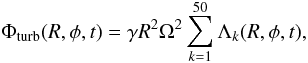 (1)with
 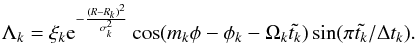 (2)In Eq. (2), ξk is a dimensionless constant parameter randomly sorted with a Gaussian distribution of unit width. Rk and φk are, respectively, the radial and azimuthal initial coordinates of the mode with wavenumber mk, σk = πRk/4mk is the radial extent of that mode, and Ωk denotes the Keplerian angular velocity at R = Rk. Both Rk and φk are randomly sorted with a uniform distribution, whereas mk is randomly sorted with a logarithmic distribution between mk = 1 and mk = 96. Following Ogihara et al. (2007), we set Λk = 0 if mk > 6 to save computing time. Each mode of wavenumber mk starts at time t = t0,k and terminates when
  , where Δtk = 0.2πRk/mkcs, cs being the sound speed, denotes the lifetime of mode with wavenumber mk. Such a value for Δtk yields a turbulence with autocorrelation timescale τc ~ Torb, where Torb is the orbital period at R = 1 (Baruteau & Lin 2010).
In Eq. (1), γ denotes the value of the turbulent forcing parameter, which controls the amplitude of the stochastic density perturbations. In the simulations presented here, we used four different values for γ, namely, γ = 6 × 10⁻⁵, 1.3 × 10⁻⁴, 1.9 × 10⁻⁴, 3 × 10⁻⁴. Given that γ is related to the effective viscous stress parameter α and the disk aspect ratio h = H/R by the relation α = 1.4 × 10²(γ/h)2 (Baruteau & Lin 2010), the last values for γ correspond to α ≅ 2 × 10⁻⁴, 10-3, 2 × 10⁻³, 5 × 10⁻³, respectively. Inviscid simulations with α = 0 were also performed for comparison.
In calculations with high values of γ, viscous stresses arising from turbulence can eventually lead to a significant change in the disk surface density profile over a few thousand orbits. This is also observed in 3D MHD simulations in which turbulence is generated by the MRI (Papaloizou & Nelson 2003). For lower values of γ, such an effect also occurs but on a much longer time scale. To examine how this affects the results of the simulations, we performed additional simulations in which the initial surface density profile is restored on a characteristic timescale τm. We followed Nelson & Gressel (2010) and solve the following equation at each time step: 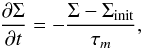 (3)where Σinit is the initial disk surface density and where τm is set to τm = 20 orbits. Such a value is lower than the viscous time scale but longer than both the dynamical time scale at the outer edge of the disk and the lifetime of the mode with wavenumber m = 1. The results of these simulations are discussed in Sect. 4.1.4.
2.2. Initial conditions
In this paper, we adopt a locally isothermal equation of state with a fixed temperature profile given by T = T0R − β where β = 1 and where T0 is the temperature at R = 1. This corresponds to a disk with constant aspect ratio h, and for most of the simulations, we chose T0 so that h = 0.05. The initial surface density profile was chosen to be Σinit(R) = Σ0R − σ with σ = 0.5 and we performed simulations with Σ0 = 2 × 10⁻⁴ and Σ0 = 4 × 10⁻⁴. Assuming that the radius R = 1 in the computational domain correponds to 5.2 AU, such values for Σ0 correspond to disks containing 0.02 M ⋆ and 0.04 M ⋆ , respectively, of gas material inside to 40 AU. No kinematic viscosity is employed in all the runs presented here.
Parameters used in the simulations.
The inner and outer planets initially evolve on circular orbits at ai = 1 and ao = 1.33, respectively, which corresponds to a configuration for which the outermost planet is initially located just outside the 3:2 MMR with the inner one. For most models, we focus on equal-mass planets with mi = mo ≤ 3.3 M⊕, where mi (mo) is the mass of innermost (outermost) planet. However, we also considered one case in which the planet mass ratio q = mi/mo is q = 1/2. The parameters for all models we conducted are summarized in Table 1. Given that the type I migration time scale τmig,p of a planet with mass mp, semimajor axis ap, and on a circular orbit with angular frequency Ωp can be estimated in the locally isothermal limit by (Paardekooper et al. 2010) 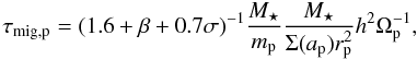 (4)we expect that equal low-mass planets embedded in our disk model will undergo convergent migration and eventually become trapped in the 3:2 resonance. For a larger initial separation between the two planets, capture in 2:1 resonance may also occur. However, test simulations have shown that, unless the disk mass is very low, differential migration is not slow enough for the planets to become trapped in that resonance. This justifies our assumption that the planets are initially located just outside the 3:2 resonance. We also notice that equal-mass planets migrating in the type I regime will undergo convergent migration provided that σ < 3/2 whereas σ > 3/2 will lead to divergent migration.
3. Theoretical expectations
In this section, we consider two low-mass planets embedded in a turbulent disk and locked in a p + 1:p mean motion resonance, and we derive the critical amplitude of the turbulent forcing γc below which the resonance would remain stable. Following Adams et al. (2008) and Rein & Papaloizou (2009), we assume that only the outermost planet experiences the torques arising from the disk. We also assume that the planets have near equal mass, in order to avoid the chaotic regime that comes into play for disparate masses (Papaloizou & Szuszkiewicz 2005). In the limit of a high damping rate for the resonance and neglecting effects from planet-planet interaction, the asymptotic value P of the probability for the resonance to be maintained is given by (Lecoanet et al. 2009) 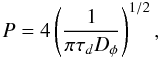 (5)where Dφ is the diffusion coefficient associated with the resonant angle diffusion, and τd is the damping timescale for the resonance angle. This equation is valid at late times
  where ω0 is the libration frequency of the resonant angles, as long as
  and
and  . From the previous equation, we can estimate the maximum value of the diffusion coefficient for the sytem to remain bound in resonance with probability P = 1. This reads as
 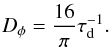 (6)As shown in Adams et al. (2008), Dφ can be related to the diffusion coefficient DH,o associated with the diffusion of the outer planet’s angular momentum as
 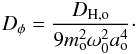 (7)For moderate eccentricities, ω0 is given by
  (8)where ei is the eccentricity of the inner planet, q0 = m0/M ⋆ , and Ωi the angular frequency of the innermost planet. In the previous equation, α = ai/ao, (j2,j4) are integers that depend on the resonance being considered, and fd(α) results from the expansion of the disturbing function. In the case of the 3:2 resonance, we have j2 = −2, j4 = −1 and αfd(α) ~ −1.54 (Murray & Dermott 1999).
In Eq. (7), DH,o can be expressed in terms of both the correlation timescale τc associated with the stochastic torques exerted on the outer planet and the standard deviation of the turbulent torque distribution σt as: 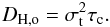 (9)As discussed in Baruteau & Lin (2010), σt takes the following form when applied to the outermost planet:
 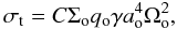 (10)where qo = mo/M ⋆ , Σo is the value of the surface density at the position of the outer planet, Ωo the angular frequency of this planet, and C is a constant. For a simulation using the same disk parameters as for model G1 and with γ = 6 × 10⁻⁵, we find C ~ 1.6 × 10², which is close to the value found by Baruteau & Lin (2010). Combining Eqs. (7), (9), and (10) gives an expression for the diffusion coefficient associated with the diffusion of the resonant angle DΦ, in terms of the value for the turbulent forcing γ. This reads as
 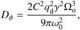 (11)with
  . Setting δω = ω0/Ωo, we can rewrite the previous expression as:
 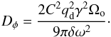 (12)We notice that, in the case where p = 1, δω is comparable to the dimensionless width of the libration zone. Using the previous equation with Eq. (6), we find that the critical value for the turbulent forcing above which the 3:2 resonance is disrupted is given by
 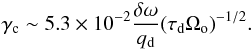 (13)In the absence of turbulent forcing, we expect the amplitude of the resonant angles to scale as
  (Peale 1976). According to Rein & Papaloizou (2009), this implies that the damping timescale of the libration amplitude τd is twice the migration timescale τmig of the whole system, namely the one composed of the two planets locked in resonance and migrating inward together. In that case, the previous equation becomes
 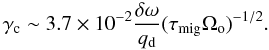 (14)In the limit where mi ~ 0, we would have τmig = τmig,o where τmig,o is the migration timescale of the outer planet, which is given by Eq. (4) with h = 0.05, σ = 0.5, and β = 1. In that case the expression for γc becomes for our disk model
 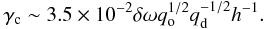 (15)To check the validity of the previous expression for γc, we performed a few N-body runs using a fifth-order Runge Kutta method. In these calculations, the forces arising from type I migration are not determined self-consistently but modelled using prescriptions for both the migration rate τap and eccentricity damping rate τep of the planets. For τap, we used
 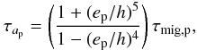 (16)where ep is the planet eccentricity and where τmig,p is given by Eq. (4) and where the numerical factor accounts for the modification of the migration rate at high eccentricities (Papaloizou & Larwood 2000). For τep we used (Tanaka & Ward 2004)
 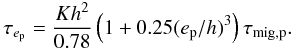 (17)In the last equation, K ~ 1.7 is a constant that was chosen in such a way that the eccentricity damping rate obtained in N-boby runs gives good agreement with what results from hydrodynamical simulations. Following Rein et al. (2010), we model the effects of turbulence as an uncorrelated noise by perturbing at each time step Δt the velocity components vi,p of each planet by
  where ξ is a random variable with a Gaussian distribution of unit width, D is the diffusion coefficient that should vary as the planets migrate, but which was fixed here to a constant value of
  .
.
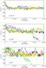 |
Fig. 1 Time evolution of the period ratio resulting from N-body runs for model G1 and for six different realizations with γ = 1.3 × 10⁻⁴, γ = 1.9 × 10⁻⁴, and γ = 3 × 10⁻⁴. |
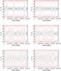 |
Fig. 2 Upper panel: time evolution of the resonant angles φ1 = 3λo − 2λi − ωi (black) and φ2 = 3λo − 2λi − ωo (red) resulting from N-body runs for model G1 and for two different realizations with γ = 1.3 × 10⁻⁴. Middle panel: same but for γ = 1.9 × 10⁻⁴. Lower panel: same but for γ = 3 × 10⁻⁴. |
In Fig. 1 we show the time evolution of the orbital period ratio for N-body simulations with parameters corresponding to model G1 and for six different realizations with γ = 1.3 × 10-4,1.9 × 10-4,3 × 10⁻⁴. For this model, we estimate δω ~ 1.9 × 10⁻³ (see Sect. 4.1.4), which leads to γc ~ 2.5 × 10⁻⁴ using Eq. (15). From Fig. 1, it appears that capture in the 3:2 MMR occurs for most of the realizations with γ ≤ 1.9 × 10⁻⁴. For two specific realizations of each value for γ we considered, the time evolution of the resonant angles φ1 = 3λo − 2λi − ωi and φ2 = 3λo − 2λi − ωo associated with the 3:2 resonance, where λi (λo) and ωi (ωo) are, respectively, the mean longitude and longitude of pericentre of the innermost (outermost) planet, is displayed in Fig. 2. Although the angles can eventually circulate for short periods of time, it is clear that the 3:2 MMR remains stable on average for γ ≤ 1.9 × 10⁻⁴. For γ = 3 × 10⁻⁴, we find that the planets pass through the 3:2 resonance in two of the six realizations performed, while the four others can eventually involve temporary capture in the 3:2 MMR. In these cases, however, the lifetime of the resonance does not exceed a few hundred orbits, as can be seen in the lower panel of Fig. 2, which displays, for γ = 3 × 10⁻⁴, the time evolution of φ1 and φ2 for two realizations in which the period ratio remains close to that corresponding to the 3:2 MMR. Therefore, the results of these N-body calculations suggest that the 3:2 MMR is only marginally stable for this value of γ, which is consistent with the aforementioned analytical estimation of γc ~ 2.5 × 10⁻⁴.
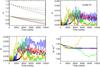 |
Fig. 3 Upper left (first) panel: time evolution of planet semi-major axes for model G1 and for γ = 0 (black line), γ = 6 × 10⁻⁵ (red line), γ = 1.3 × 10⁻⁴ (blue), γ = 1.9 × 10⁻⁴ (green), and γ = 3 × 10⁻⁴ (orange). Upper right (second) panel: time evolution of the inner planet eccentricity. Third panel: time evolution of the outer planet eccentricity. Fourth panel: time evolution of the period ratio. Simulations were performed with GENESIS. |
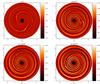 |
Fig. 4 This figure shows, for model G1, snapshots of the perturbed surface density of the disk for γ = 0 (first panel), γ = 6 × 10⁻⁵ (second panel), γ = 1.3 × 10⁻⁴ (third panel), and γ = 1.9 × 10⁻⁴ (fourth panel). |
4. Results of hydrodynamical simulations
For equal-mass planets (q = 1), results of hydrodynamical simulations suggest that capture in 3:2 resonance can occur in turbulent disks for which the level of turbulence is relatively weak. For systems with q ≤ 1/2, however, it appears that trapping in the 3:2 resonance is only maintained when the disk is close to being inviscid.
4.1. Models with q = 1
For inviscid simulations with equal low-mass planets, the ability for the two planets to become trapped in the 3:2 resonance depends mainly on the planets’ relative migration rate which scales as h-2. For model G3 (h = 0.04), we find that capture in 3:2 resonance does not occur in that case because the relative migration timescale is shorter than the libration period corresponding to that resonance. For other models with h = 0.05, however, it appears that the system can enter into a 3:2 commensurability that remains stable for the duration of the simulation, which generally covers ~104 orbits at R = 1. This occurs not only for laminar disks, but also for turbulent disks provided that the value for the turbulent forcing is not too large. For example, we find that the 3:2 commensurability is maintained in most of the turbulent runs with γ ≤ 1.3 × 10⁻⁴ in models G1 and G2, whereas this occurs in model G4 provided that γ ≤ 6 × 10⁻⁵. Below we describe the results of the simulations with q = 1 in more detail and use model G1 to illustrate how the evolution depends on the value for the forcing parameter γ.
4.1.1. Orbital evolution
The time evolution of the planets’ semi-major axes, eccentricities, and period ratio corresponding to model G1 and for one realization of the different values of γ we considered are depicted in Fig. 3. In each case, the period ratio is observed to decrease initially, suggesting that early evolution involves convergent migration of the two planets. Not surprisingly, a tendency for the planets to undergo a monotonic inward migration is observed at the beginning of the simulations with the lowest values of γ whereas these are more influenced by stochastic forcing for γ ≥ 1.9 × 10⁻⁴. This is because the amplitude of the turbulent density fluctuations is typically stronger than that of the planet’s wake for simulations with γ ≥ 1.9 × 10⁻⁴, as shown in Fig. 4, which displays snapshots of the perturbed surface density of the disk for different values of γ.
The semimajor axis evolution also reveals a clear tendency for lower migration rates with increasing γ, which is an effect arising from the desaturation of the horseshoe drag by turbulence (Baruteau & Lin 2010). As γ increases, the disk torques are indeed expected to increase from the differential Lindblad torque, obtained for γ = 0, up to the fully unsaturated torque, which is maintained for α ~ 0.16(mi/M ∗ )3/2h-4 (Baruteau & Lin 2010). For h = 0.05, such a value for α corresponds to γ ~ 1.2 × 10⁻⁴. For higher values of γ, however, we expect the torques to slightly decrease with increasing γ owing to a cut-off of the horseshoe drag arising when the diffusion timescale across the horseshoe region is smaller than the horseshoe U-turn time (Baruteau & Lin 2010).
This can be confirmed by inspecting the evolution of the running-time averaged torques exerted on both planets. They are presented in Fig. 5. Up to a time of approximately ~103 orbits and for γ ≤ 1.3 × 10⁻⁴, the torques are observed to increase with increasing γ, while they decrease for higher values of γ. This agrees very well with the expectation that the fully unsaturated torque is reached for γ = 1.2 × 10⁻⁴. At later times, however, the torques obtained in simulations with γ ≥ 1.9 × 10⁻⁴ can eventually exceed those computed in runs with γ ≤ 1.3 × 10⁻⁴. We suggest that this is related to the fact that the disk surface density tends to be significantly modified at the planet positions at high turbulence level. This is illustrated in Fig. 6, which shows the disk surface density profile at t = 2000 orbits for the different values of γ we considered. Here the inner and outer planets are located at ai ~ 0.98 and ao ~ 1.25, respectively. It is interesting to note that, for γ = 3 × 10⁻⁴, the outer planet tends to evolve in a region of positive surface density gradient where the corotation torque is positive, in such a way that the torque exerted on that planet can become higher than that exerted on the inner one. This effect is responsible for the increase of period ratio observed at late times in simulations with γ ≥ 1.9 × 10⁻⁴.
4.1.2. Eccentricity evolution
For model G1, examination of the early planets’ eccentricities evolution displayed in Fig. 3 shows a clear tendency for higher eccentricities with increasing the value for γ, which agrees with the expectation that turbulence is a source of eccentricity driving (Nelson 2005). This can be confirmed by inspecting the theoretical change of the inner planet eccentricity dei/dt, which can be computed using the following expression (Burns 1976):  (18)where E = −G(M ⋆ + mi)/2ai is the specific energy of the inner planet,
  its specific angular momentum, Ḣ the torque exerted by the disk, and Ė the power of the force exerted by the disk on the planet. The early time evolution of dei/dt is displayed for this model and for the different values of γ we considered in the upper panel of Fig. 7. It clearly demonstrates that, compared with the laminar run, the theoretical rate of change of ei is higher in turbulent runs and that it increases with increasing the value for γ.
Also, inspection of the lower panel of Fig. 7 reveals that, compared with model G1 in which mi = mo = 3.3M⊕ and Σ0 = 2 × 10⁻⁴, the disk induced eccentricity damping is weaker in model G4 for which mi = mo = 1.6M⊕. This is due to the damping of eccentricity at coorbital Lindblad resonances scaling linearly with planet mass (Nelson 2005). Given that this damping also scales with disk mass, this explains why the disk induced eccentricity damping is stronger in model G2 in which Σ0 = 4 × 10⁻⁴.
4.1.3. Time evolution of the resonant angles
As mentioned above, we find that a stable 3:2 commensurability generally forms for model G1 and for γ ≤ 1.3 × 10⁻⁴, which can be confirmed by inspecting the upper panel of Fig. 8, which displays the time evolution of the period ratio for four different realizations with this value of γ. However, as one can see in the lower panel of Fig. 8, such a resonance is observed to break at late times for all the realizations performed with γ ≥ 1.9 × 10⁻⁴. Comparing Fig. 8 and the two upper panels in Fig. 1, we see that the results of these hydrodynamical simulations are at first glance in good agreement with those of N-body runs. Moreover, it is interesting to note that, in some runs, planets that leave the 3:2 resonance can eventually pass through that resonance again at later times or other commensurabilities like the 2:1 resonance.
 |
Fig. 5 Upper panel: time evolution of the running-time averaged torques exerted on the inner planet for model G1 and for γ = 0 (black line), γ = 6 × 10⁻⁵ (red line), γ = 1.3 × 10⁻⁴ (blue), γ = 1.9 × 10⁻⁴ (green), and γ = 3 × 10⁻⁴ (orange). Lower panel: same but for the outer planet. |
A similar outcome is observed in model G2, which had a value of Σ0 = 4 × 10⁻⁴. This arises because both the turbulent torque and the damping rate of the libration amplitude scale linearly with Σ0. For model G4 however, which had Σ0 = 2 × 10⁻⁴ and mi = mo = 1.6M⊕, the 3:2 resonance is disrupted in the run with γ = 1.3 × 10⁻⁴ because the damping rate is smaller for this model. For a single realization for each value of γ, the evolution of the period ratio for models G2 and G4 is displayed in Fig. 9.
In the two upper panels of Fig. 10 we show the time evolution of the resonant angles associated with the 3:2 resonance for model G1 and for two realizations with γ = 6 × 10⁻⁵ and γ = 1.3 × 10⁻⁴. For γ = 6 × 10⁻⁵, the 3:2 resonance is established at t ~ 1800 orbits, while it forms at t ~ 2000 orbits for the calculation with γ = 1.3 × 10⁻⁴. This is consistent with the tendency, for moderate values of γ, of migration rates to decrease with increasing γ. As illustrated in the second and third panels of Fig. 3, resonant capture makes the eccentricities of both planets grow rapidly before they saturate at values of ei ~ eo ~ 0.01 in the run with γ = 6 × 10⁻⁵. As discussed in Sect. 4.1.2, these tend to be larger when γ = 1.3 × 10⁻⁴, with the eccentricities reaching peak values of ei ~ 0.02 and eo ~ 0.015.
 |
Fig. 6 Disk surface density profile at t = 2000 orbits for model G1 and for γ = 0 (black line), γ = 6 × 10⁻⁵ (red line), γ = 1.3 × 10⁻⁴ (blue), γ = 1.9 × 10⁻⁴ (green), and γ = 3 × 10⁻⁴ (orange). |
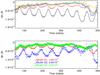 |
Fig. 7 Upper panel: time evolution of the theoretical change of the inner planet eccentricity dei/dt given by Eq. (18) for model G1 and for γ = 0 (black line), γ = 6 × 10⁻⁵ (red line), γ = 1.3 × 10⁻⁴ (blue), γ = 1.9 × 10⁻⁴ (green), and γ = 3 × 10⁻⁴ (orange). Lower panel: same but for γ = 6 × 10⁻⁵, and models G1 (red), G2 (blue), and G4 (green). |
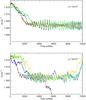 |
Fig. 8 Upper panel: time evolution of the period ratio for model G1 and for four different realizations with γ = 1.3 × 10⁻⁴. Lower panel: same but for γ = 1.9 × 10⁻⁴. Simulations were performed with GENESIS. |
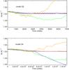 |
Fig. 9 Upper panel: time evolution of the period ratio for model G2 and for γ = 0 (black line), γ = 6 × 10⁻⁵ (red), γ = 1.3 × 10⁻⁴ (blue), γ = 1.9 × 10⁻⁴ (green) and γ = 3 × 10⁻⁴ (orange). Lower panel: same but for model G4. Simulations were performed with GENESIS. |
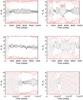 |
Fig. 10 Upper panel: time evolution of the resonant angles φ1 = 3λo − 2λi − ωi (black) and φ2 = 3λo − 2λi − ωo (red) for model G1 with γ = 6 × 10⁻⁵ (left) and γ = 1.3 × 10⁻⁴ (right). Middle panel: same but for model G2. Lower panel: same but for model G4. |
Not surprisingly, there is a clear trend for the amplitude of the resonant angles to increase with increasing the value of γ in model G1. For the run with γ = 6 × 10⁻⁵, the angles spread slightly until t ~ 5 × 10³ orbits before their amplitude continuously decreases with time. This indicates that on long timescales damping of the resonant angles through migration tends to overcome diffusion effects. When γ = 1.3 × 10⁻⁴, however, periods of cyclic variations in the resonant angles can be seen with the angles librating with high amplitude before being subsequently damped. Given that in the absence of turbulent forcing, the libration amplitude should decrease as  (Peale 1976), we would expect the 3:2 resonance to be maintained for γ ≤ 1.3 × 10⁻⁴, on much longer timescales than those covered by the simulations.
For two realizations with γ = 6 × 10⁻⁵ and γ = 1.3 × 10⁻⁴, the evolution of both φ1 and φ2 for models G2 and G4 is displayed in the middle and lower panels of Fig. 10, respectively. In comparison with model G1, the resonant angles librate with slightly higher amplitudes in model G2 and can eventually start oscillations between periods of circulation and libration in the run with γ = 1.3 × 10⁻⁴. Again this arises because the turbulent density fluctuations are stronger in this model than in model G1. In model G4 however, the 3:2 resonance is maintained for only ~ 3 × 10³ orbits when γ = 1.3 × 10⁻⁴, which indicates that for this model the damping rate is too weak for this resonance to remain stable.
4.1.4. Comparison with analytics
We now examine how the results of the simulations described above compare with the expectations discussed in Sect. 3. For model G1, we can estimate the libration frequency ω0 using Eq. (8) in conjunction with the results from this model shown in Fig. 3. Adopting the inviscid simulation as a fiducial case, we have ai = 0.9, ao = 1.17, and ei = 0.01 at t ~ 4000 orbits, which leads to δω = ω0/Ωo ~ 1.9 × 10⁻³. Moreover, the migration timescale of the system was estimated to τmig ~ 3.3 × 10⁴ orbits from the results of this simulation. Using Eq. (14) which gives the value for γc as a function of τmig, we can then provide an analytical estimate  of the critical amplitude for the turbulent forcing above which the 3:2 resonance should be disrupted. For this model, this critical value is estimated to be
  , while Eq. (15) predicts
  . Returning to Fig. 8, we see that the results of the simulations performed with GENESIS suggest that 1.3 × 10⁻⁴ ≤ γc < 1.9 × 10⁻⁴ for this model, which is clearly in broad agreement with the previous analytical estimate. We note, however, that both simulations performed with FARGO and additional runs in which a roughly constant surface density profile is maintained (see Sect. 2.1) produced slightly different results since we find 6 × 10⁻⁵ ≤ γc < 1.3 × 10⁻⁴ in these cases. The small difference exhibited by our two codes is apparently because turbulence induces changes in the surface density profile that are slightly different. In FARGO, the disk density at the position of the inner planet is slightly higher than with GENESIS, while it is slightly lower at the position of the outer planet.
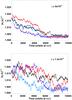 |
Fig. 11 Upper panel: time evolution of the period ratio for model G1 and for four runs with γ = 6 × 10⁻⁵ and in which Eq. (3) is solved at each time step . Lower panel: same but for γ = 1.3 × 10⁻⁴. Simulations were performed with FARGO. |
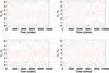 |
Fig. 12 Time evolution for model G1 and for four different realizations of the resonant angles φ1 = 3λo − 2λi − ωi (black) and φ2 = 3λo − 2λi − ωo (red) for γ = 1.3 × 10⁻⁴ and when Eq. (3) is solved at each time step. |
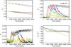 |
Fig. 13 Upper left (first) panel: time evolution of planet semi-major axes for model G5 and for γ = 0 (black line), γ = 6 × 10⁻⁵ (red line), γ = 1.3 × 10⁻⁴ (blue), γ = 1.9 × 10⁻⁴ (green), and γ = 3 × 10⁻⁴ (orange). Upper right (second) panel: time evolution of the inner planet ecentricity. Third panel: time evolution of the outer planet eccentricity. Fourth panel: time evolution of the period ratio (ao/ai)1.5. Simulations were performed with GENESIS. |
For calculations in which Eq. (3) is solved at each time step, the time evolution of the period ratio for four realizations with γ = 6 × 10⁻⁵ and γ = 1.3 × 10⁻⁴ is displayed in Fig. 11. In that case, all the realizations performed with γ = 6 × 10⁻⁵ result in the formation of the 3:2 resonance, whereas for γ = 1.3 × 10⁻⁴, two of the four realizations resulted in capture in that resonance by the end of the run. For γ = 1.3 × 10⁻⁴, the time evolution of the resonant angles associated with the 3:2 resonance is displayed in Fig. 12. Compared with previous runs in which the surface density profile was altered by turbulence, we see that capture in resonance tends to occur later in runs where a roughly constant surface density profile is maintained. This occurs because the disk density at the position of the inner planet tends to be higher in runs where the initial disk surface density profile is restored, leading to a slower differential migration between the two planets.
For other models, repeating the previously described procedure leads to analytical estimates of  for model G2 and
  for model G4. Given that the simulations performed with GENESIS indicate that 1.3 × 10⁻⁴ ≤ γc < 1.9 × 10⁻⁴ and 6 × 10⁻⁵ ≤ γc < 1.3 × 10⁻⁴ for models G2 and G4, respectively, we see that again the previous analytical estimates compare reasonably well with the results of our simulations.
4.2. Model with q = 1/2
For systems with q = 1/2, the results of the simulations indicate that the 3:2 resonance can only be maintained in cases where the disk is close to being inviscid. Figure 13 shows the results for model G5 in which mi = 1.6 M⊕ and mo = 3.3 M⊕ and for a single realization of the different values of γ we considered. From left to right and from top to bottom, the panels display the time evolution of the planets’ semi-major axes, eccentricity of the inner planet, eccentricity of the outer one, and period ratio. The evolution of semi-major axes shows strong similarities with that of model G1, with the migration rates of the planets observed to decrease with increasing the value for γ, as discussed in Sect. 4.1.1.
Because of stochastic density fluctuations, the planets’ eccentricities are highly variable quantities, and a clear trend of higher eccentricities for higher values of γ is again observed at the beginning of the simulations. For γ = 0, the time evolution of the period ratio shows that trapping in the 3:2 resonance occurs at t ~ 103 orbits. This resonant interaction causes eccentricity growth for both planets with the eccentricities of the inner and outer planets reaching peak values of ei ~ 0.035 and eo ~ 0.02, respectively, although convergence is not fully established at the end of the simulation. Comparing Figs. 3 and 13, we see that the period ratio oscillates with greater amplitude in model G5, thereby indicating that resonant locking is weaker. This arises because, compared with model G1, the relative migration rate is higher for that model. Here, it is worthwhile noticing that on timescales longer that those covered by the simulations, it is not clear whether the planets will remain bound in the 3:2 resonance since for disparate planet masses as is the case for model G5, we expect the dynamics of the system to be close to the chaotic regime even for γ = 0 (Papaloizou & Szuszkiewicz 2005).
For turbulent runs, we find that the planets become temporarily trapped in the 3:2 resonance but in each case, the final outcome appears to be disruption of that resonance. Not surprisingly, the survival time of the 3:2 resonance tends to increase with decreasing the value of γ. For these realizations, the lifetimes of the resonance are estimated to be ~1500 orbits for γ = 6 × 10⁻⁵, ~ 2 × 10³ orbits for γ = 1.3 × 10⁻⁴, and ~103 orbits for γ = 1.9 × 10⁻⁴. The slightly longer lifetime of the resonance obtained in the run with γ = 1.3 × 10⁻⁴ arises because of the stochastic nature of the problem.
In Fig. 14 is displayed for two runs with γ = 6 × 10⁻⁵ and γ = 1.3 × 10⁻⁴, the evolution of the resonant angles associated with the 3:2 resonance. In comparison with models in which q = 1, there is a clear tendency for them to librate with higher amplitude.Therefore, for models with disparate planet masses, the origin of the disruption of the 3:2 resonance in turbulent runs is likely to be related to the combined effect of diffusion of the resonant angles plus high libration amplitudes because the resonance is weaker.
For γ ≥ 6 × 10⁻⁵, we cannot rule out the possibility that the planets would become locked in stronger p + 1:p resonances with p ≥ 3. To investigate this issue in more detail, we performed an additional set of simulations in which, for each value of γ we considered, the outer planet was initially located just outside the 4:3 resonance with the inner one. When the 4:3 resonance was found to be unstable, we performed an additional run but with an initial separation between the two planets slightly larger than the one corresponding to the 5:4 resonance. If the 5:4 resonance is not maintained, we repeated the procedure described above until a stable p + 1:p commensurability eventually formed. Because performing several realizations for each value of γ would require a large suite of simulations, we considered only one single realization for each value of γ.
Figure 15 illustrates how the established resonance depends on the value for the turbulent forcing. Not surprisingly, a clear trend toward forming stronger p + 1:p resonances with increasing γ is observed. For γ = 6 × 10⁻⁵, the system enters in a stable 4:3 resonance, while for γ = 1.3 × 10⁻⁴, the planets instead become locked in the 5:4 resonance. For the runs with γ = 1.9 × 10⁻⁴ and γ = 3 × 10⁻⁴, however, the planets become temporarily trapped in the 8:7 resonance, but in each case this commensurability is subsequently lost with the planets undergoing divergent migration. In that case, it is interesting to note that the system is close to the stability limit since for planets in the Earth mass range, as is the case here, we expect resonance overlap to occur for p ≥ 8 (Papaloizou & Szuszkiewicz 2005). Therefore, we can reasonably suggest that, for such values of γ, super-Earths with mass ratio q = mi/mo < 1/2 may not be able to become trapped in a stable mean motion resonance and may eventually suffer close encouters.
5. Discussion and conclusion
In this paper we have presented the results of hydrodynamic simulations aimed at studying the evolution of a system composed of two planets in the Earth mass range and embedded in a turbulent protoplanetary disk. We employed the turbulence model of Laughlin et al. (2004), modified by Baruteau & Lin (2010), in which a turbulent potential corresponding to the superposition of multiple wave-like modes is applied to the disk. We focused on a scenario in which the outermost planet is initially located just outside the 3:2 resonance and investigated how the evolution depends on both the planet mass ratio q and the value for the turbulent forcing parameter γ.
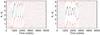 |
Fig. 14 Time evolution of the resonant angles φ1 = 3λo − 2λi − ωi (black), φ2 = 3λo − 2λi − ωo (red) for model G1 with γ = 6 × 10⁻⁵ (left panel), and γ = 1.3 × 10⁻⁴ (right panel). |
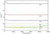 |
Fig. 15 Period ratio between the two planets for model G5 with γ = 0 (black line), γ = 6 × 10⁻⁵ (red), γ = 1.3 × 10⁻⁴ (blue), γ = 1.9 × 10⁻⁴ (green), and γ = 3 × 10⁻⁴ (orange). Simulations were performed with GENESIS. |
The results of the simulations indicate that, for systems with equal mass planets, a 3:2 resonance can be maintained in the presence of weak turbulence. For instance, for two planets with equal mass 3.3 M⊕, we found that the 3:2 resonance is stable in runs with γ ≤ 1.9 × 10⁻⁴, which corresponds to values for the effective viscous stress parameter of α ≲ 2 × 10⁻³. Such a value was found to compare fairly well with what results from both analytical estimations and preliminary N-body runs. For systems with a planet mass ratio q ≤ 1/2, however, it appears that a 3:2 resonance can remain stable only when the disk is close to being inviscid. In turbulent disks, however, the outcome depends strongly on the value for γ:
i): For 6 × 10⁻⁵ ≤ γ ≤ 1.3 × 10⁻⁴ (equivalent to 2 × 10⁻⁴ ≲ α ≲ 10-3), the planets tend to become locked in stronger p + 1:p resonances, with p increasing as the value for γ increases.
ii): When γ ≥ 1.9 × 10⁻⁴ (equivalent to α ≥ 2 × 10⁻³), we found that the planets can become temporarily trapped in a 8:7 commensurability, but this resonance is disrupted at later times, and no stable resonance is formed.
Given that the volume-averaged stress parameter deduced from MHD simulations is typically α ~ 5 × 10⁻³ (Papaloizou & Nelson 2003; Nelson 2005), these results suggest that mean motion resonances between planets in the Earth’s mass range are likely to be disrupted in the active zones of protoplanetary disks. For relatively low levels of turbulence, however, as is the case for a dead-zone (Gammie 1996), a resonance can be maintained for moderate values of the planet mass ratio.Such a scenario is broadly consistent with the preliminary analysis of ~170 multi-planetary systems candidates recently detected by Kepler (Lissauer et al. 2011) and which suggests that only a few of the observed adjacent pairings are either in or near a MMR. However, examination of the slope of the cumulative distribution of period ratios (Fig. 7 of Lissauer et al. 2011) also reveals an excess of planets with period ratios corresponding to the 2:1 or 3:2 commensurabilities. In that case, it appears that the neighbouring planet candidates have masses within 20% of each other. This clearly supports our findings that, in disks with moderate levels of turbulence, MMRS are stable provided the mass ratio between the neighbouring planets is close to unity.
Since turbulence has a significant impact on the capture of two planets in the Earth mass range, it will be of interest to examine this issue using 3D MHD simulations, which eventually include the presence of a dead-zone. We will address this issue in a future paper.
References
- Adams, F. C., Laughlin, G., & Bloch, A. M. 2008, ApJ, 683, 1117 [NASA ADS] [CrossRef] [Google Scholar]
- Balbus, S. A., & Hawley, J. F. 1991, ApJ, 376, 214 [NASA ADS] [CrossRef] [Google Scholar]
- Baruteau, C., & Lin, D. N. C. 2010, ApJ, 709, 759 [NASA ADS] [CrossRef] [Google Scholar]
- Brandenburg, A., Nordlund, A., Stein, R. F., & Torkelsson, U. 1996, ApJ, 458, L45 [NASA ADS] [CrossRef] [Google Scholar]
- Burns, J. A. 1976, Am. J. Phys., 44, 944 [NASA ADS] [CrossRef] [Google Scholar]
- Charbonneau, D., Berta, Z. K., Irwin, J., et al. 2009, Nature, 462, 891 [NASA ADS] [CrossRef] [PubMed] [Google Scholar]
- Cresswell, P., & Nelson, R. P. 2006, A&A, 450, 833 [NASA ADS] [CrossRef] [EDP Sciences] [Google Scholar]
- De Val-Borro, M., Edgar, R. G., Artymowicz, P., et al. 2006, MNRAS, 370, 529 [NASA ADS] [CrossRef] [Google Scholar]
- Fromang, S., & Nelson, R. P. 2009, A&A, 496, 597 [NASA ADS] [CrossRef] [EDP Sciences] [Google Scholar]
- Fromang, S., & Papaloizou, J. 2006, A&A, 452, 751 [NASA ADS] [CrossRef] [EDP Sciences] [Google Scholar]
- Gammie, C. F. 1996, ApJ, 457, 355 [NASA ADS] [CrossRef] [Google Scholar]
- Hawley, J. F., Gammie, C. F., & Balbus, S. A. 1996, ApJ, 464, 690 [NASA ADS] [CrossRef] [Google Scholar]
- Konacki, M., & Wolszczan, A. 2003, ApJ, 591, L147 [NASA ADS] [CrossRef] [Google Scholar]
- Ketchum, J. A., Adams, F. C., & Bloch, A. M. 2011, ApJ, 726, 53 [NASA ADS] [CrossRef] [Google Scholar]
- Laughlin, G., Steinacker, A., & Adams, F. C. 2004, ApJ, 608, 489 [NASA ADS] [CrossRef] [Google Scholar]
- Lecoanet, D., Adams, F. C., & Bloch, A. M. 2009, ApJ, 692, 659 [NASA ADS] [CrossRef] [Google Scholar]
- Léger, A., Rouan, D., Schneider, J., et al. 2009, A&A, 506, 287 [NASA ADS] [CrossRef] [EDP Sciences] [MathSciNet] [Google Scholar]
- Lissauer, J. J., Ragozzine, D., Fabrycky, D. C., et al. 2011 [arXiv:1102.0543] [Google Scholar]
- Masset, F. 2000, A&AS, 141, 165 [NASA ADS] [CrossRef] [EDP Sciences] [Google Scholar]
- Mayor, M., Udry, S., Lovis, C., et al. 2009, A&A, 493, 639 [NASA ADS] [CrossRef] [EDP Sciences] [Google Scholar]
- McNeil, D., Duncan, M., & Levison, H. F. 2005, AJ, 130, 2884 [NASA ADS] [CrossRef] [Google Scholar]
- Murray, C. D., & Dermott, S. F. 1999, Solar system dynamics, ed. C. D. Murray [Google Scholar]
- Nelson, R. P. 2005, A&A, 443, 1067 [NASA ADS] [CrossRef] [EDP Sciences] [Google Scholar]
- Nelson, R. P., & Gressel, O. 2010, MNRAS, 409, 639 [NASA ADS] [CrossRef] [Google Scholar]
- Nelson, R. P., Papaloizou, J. C. B., Masset, F., & Kley, W. 2000, MNRAS, 318, 18 [NASA ADS] [CrossRef] [Google Scholar]
- Ogihara, M., Ida, S., & Morbidelli, A. 2007, Icarus, 188, 522 [NASA ADS] [CrossRef] [Google Scholar]
- Paardekooper, S.-J., Baruteau, C., Crida, A., & Kley, W. 2010, MNRAS, 401, 1950 [NASA ADS] [CrossRef] [Google Scholar]
- Papaloizou, J. C. B., & Larwood, J. D. 2000, MNRAS, 315, 823 [NASA ADS] [CrossRef] [Google Scholar]
- Papaloizou, J. C. B., & Nelson, R. P. 2003, MNRAS, 339, 983 [NASA ADS] [CrossRef] [Google Scholar]
- Papaloizou, J. C. B., & Szuszkiewicz, E. 2005, MNRAS, 363, 153 [NASA ADS] [CrossRef] [MathSciNet] [Google Scholar]
- Peale, S. J. 1976, ARA&A, 14, 215 [NASA ADS] [CrossRef] [Google Scholar]
- Press, W. H., Teukolsky, S. A., Vetterling, W. T., & Flannery, B. P. 1992, 2nd edn. (Cambridge: University Press) [Google Scholar]
- Queloz, D., Bouchy, F., Moutou, C., et al. 2009, A&A, 506, 303 [NASA ADS] [CrossRef] [EDP Sciences] [Google Scholar]
- Rein, H., & Papaloizou, J. C. B. 2009, A&A, 497, 595 [NASA ADS] [CrossRef] [EDP Sciences] [Google Scholar]
- Rein, H., Lesur, G., & Leinhardt, Z. M. 2010, A&A, 511, A69 [NASA ADS] [CrossRef] [EDP Sciences] [Google Scholar]
- Sicilia-Aguilar, A., Hartmann, L. W., Briceño, C., Muzerolle, J., & Calvet, N. 2004, AJ, 128, 805 [NASA ADS] [CrossRef] [Google Scholar]
- Tanaka, H., & Ward, W. R. 2004, ApJ, 602, 388 [NASA ADS] [CrossRef] [Google Scholar]
- Tanaka, H., Takeuchi, T., & Ward, W. R. 2002, ApJ, 565, 1257 [NASA ADS] [CrossRef] [Google Scholar]
- Terquem, C., & Papaloizou, J. C. B. 2007, ApJ, 654, 1110 [NASA ADS] [CrossRef] [Google Scholar]
- van Leer, B. 1977, J. Comp. Phys., 23, 276 [Google Scholar]
- Ward, W. R. 1997, Icarus, 126, 261 [NASA ADS] [CrossRef] [Google Scholar]
All Tables
All Figures
|
Fig. 1 Time evolution of the period ratio resulting from N-body runs for model G1 and for six different realizations with γ = 1.3 × 10⁻⁴, γ = 1.9 × 10⁻⁴, and γ = 3 × 10⁻⁴. |
| In the text | |
|
Fig. 2 Upper panel: time evolution of the resonant angles φ1 = 3λo − 2λi − ωi (black) and φ2 = 3λo − 2λi − ωo (red) resulting from N-body runs for model G1 and for two different realizations with γ = 1.3 × 10⁻⁴. Middle panel: same but for γ = 1.9 × 10⁻⁴. Lower panel: same but for γ = 3 × 10⁻⁴. |
| In the text | |
|
Fig. 3 Upper left (first) panel: time evolution of planet semi-major axes for model G1 and for γ = 0 (black line), γ = 6 × 10⁻⁵ (red line), γ = 1.3 × 10⁻⁴ (blue), γ = 1.9 × 10⁻⁴ (green), and γ = 3 × 10⁻⁴ (orange). Upper right (second) panel: time evolution of the inner planet eccentricity. Third panel: time evolution of the outer planet eccentricity. Fourth panel: time evolution of the period ratio. Simulations were performed with GENESIS. |
| In the text | |
|
Fig. 4 This figure shows, for model G1, snapshots of the perturbed surface density of the disk for γ = 0 (first panel), γ = 6 × 10⁻⁵ (second panel), γ = 1.3 × 10⁻⁴ (third panel), and γ = 1.9 × 10⁻⁴ (fourth panel). |
| In the text | |
|
Fig. 5 Upper panel: time evolution of the running-time averaged torques exerted on the inner planet for model G1 and for γ = 0 (black line), γ = 6 × 10⁻⁵ (red line), γ = 1.3 × 10⁻⁴ (blue), γ = 1.9 × 10⁻⁴ (green), and γ = 3 × 10⁻⁴ (orange). Lower panel: same but for the outer planet. |
| In the text | |
|
Fig. 6 Disk surface density profile at t = 2000 orbits for model G1 and for γ = 0 (black line), γ = 6 × 10⁻⁵ (red line), γ = 1.3 × 10⁻⁴ (blue), γ = 1.9 × 10⁻⁴ (green), and γ = 3 × 10⁻⁴ (orange). |
| In the text | |
|
Fig. 7 Upper panel: time evolution of the theoretical change of the inner planet eccentricity dei/dt given by Eq. (18) for model G1 and for γ = 0 (black line), γ = 6 × 10⁻⁵ (red line), γ = 1.3 × 10⁻⁴ (blue), γ = 1.9 × 10⁻⁴ (green), and γ = 3 × 10⁻⁴ (orange). Lower panel: same but for γ = 6 × 10⁻⁵, and models G1 (red), G2 (blue), and G4 (green). |
| In the text | |
|
Fig. 8 Upper panel: time evolution of the period ratio for model G1 and for four different realizations with γ = 1.3 × 10⁻⁴. Lower panel: same but for γ = 1.9 × 10⁻⁴. Simulations were performed with GENESIS. |
| In the text | |
|
Fig. 9 Upper panel: time evolution of the period ratio for model G2 and for γ = 0 (black line), γ = 6 × 10⁻⁵ (red), γ = 1.3 × 10⁻⁴ (blue), γ = 1.9 × 10⁻⁴ (green) and γ = 3 × 10⁻⁴ (orange). Lower panel: same but for model G4. Simulations were performed with GENESIS. |
| In the text | |
|
Fig. 10 Upper panel: time evolution of the resonant angles φ1 = 3λo − 2λi − ωi (black) and φ2 = 3λo − 2λi − ωo (red) for model G1 with γ = 6 × 10⁻⁵ (left) and γ = 1.3 × 10⁻⁴ (right). Middle panel: same but for model G2. Lower panel: same but for model G4. |
| In the text | |
|
Fig. 11 Upper panel: time evolution of the period ratio for model G1 and for four runs with γ = 6 × 10⁻⁵ and in which Eq. (3) is solved at each time step . Lower panel: same but for γ = 1.3 × 10⁻⁴. Simulations were performed with FARGO. |
| In the text | |
|
Fig. 12 Time evolution for model G1 and for four different realizations of the resonant angles φ1 = 3λo − 2λi − ωi (black) and φ2 = 3λo − 2λi − ωo (red) for γ = 1.3 × 10⁻⁴ and when Eq. (3) is solved at each time step. |
| In the text | |
|
Fig. 13 Upper left (first) panel: time evolution of planet semi-major axes for model G5 and for γ = 0 (black line), γ = 6 × 10⁻⁵ (red line), γ = 1.3 × 10⁻⁴ (blue), γ = 1.9 × 10⁻⁴ (green), and γ = 3 × 10⁻⁴ (orange). Upper right (second) panel: time evolution of the inner planet ecentricity. Third panel: time evolution of the outer planet eccentricity. Fourth panel: time evolution of the period ratio (ao/ai)1.5. Simulations were performed with GENESIS. |
| In the text | |
|
Fig. 14 Time evolution of the resonant angles φ1 = 3λo − 2λi − ωi (black), φ2 = 3λo − 2λi − ωo (red) for model G1 with γ = 6 × 10⁻⁵ (left panel), and γ = 1.3 × 10⁻⁴ (right panel). |
| In the text | |
|
Fig. 15 Period ratio between the two planets for model G5 with γ = 0 (black line), γ = 6 × 10⁻⁵ (red), γ = 1.3 × 10⁻⁴ (blue), γ = 1.9 × 10⁻⁴ (green), and γ = 3 × 10⁻⁴ (orange). Simulations were performed with GENESIS. |
| In the text | |
Current usage metrics show cumulative count of Article Views (full-text article views including HTML views, PDF and ePub downloads, according to the available data) and Abstracts Views on Vision4Press platform.
Data correspond to usage on the plateform after 2015. The current usage metrics is available 48-96 hours after online publication and is updated daily on week days.
Initial download of the metrics may take a while.