| Issue |
A&A
Volume 531, July 2011
|
|
|---|---|---|
| Article Number | A168 | |
| Number of page(s) | 11 | |
| Section | Planets and planetary systems | |
| DOI | https://doi.org/10.1051/0004-6361/201116529 | |
| Published online | 08 July 2011 | |
Thermal properties of the asteroid (2867) Steins as observed by VIRTIS/Rosetta
1
LESIA, Observatoire de Paris, CNRS, UPMC, Université Paris-Diderot, 5 place Jules Janssen, 92195 Meudon, France
e-mail: This email address is being protected from spambots. You need JavaScript enabled to view it.
2
INAF-IFSI Istituto di Fisica dello Spazio Interplanetario, via del Fosso del Cavaliere 100, 00133 Roma, Italy
3
INAF-IASF Istituto di Astrofisica Spaziale e Fisica Cosmica, via del Fosso del Cavaliere 100, 00133 Roma, Italy
Received: 17 January 2011
Accepted: 1 May 2011
Abstract
Context. To investigate thermal properties of the small asteroid (2867) Steins, we analyzed its surface thermal emission measured by the VIRTIS instrument during the Rosetta spacecraft (ESA) flyby that occurred in September 2008. VIRTIS performed the first thermal mapping of an asteroid surface.
Aims. We determine the thermal properties of different locations at the surface of Steins and the thermal inertia is constrained by measuring the variations of the surface temperature for different local times.
Methods. The surface temperature on the morning side of Steins is measured by inverting IR spectra between 4 and 5 microns acquired by the VIRTIS-M instrument onboard the Rosetta spacecraft. It is then compared to the theoretical temperatures obtained with a thermophysical model assuming either a smooth or rough surface. The heat conduction is computed radially into the first millimeters below the surface assuming a non-zero thermal inertia. The shape of the asteroid is reproduced by a 3D shape model composed of thousands of independent facets. We then compare both observed and computed temperatures within the footprint at different local times.
Results. The observed temperatures are reproduced by a thermal inertia Γ = 110 ± 13 J m-2 K-1 s−1/2 for a smooth surface but some discrepancies remain between data and the thermal model at high incidence angles on the morning side near the terminator. This suggests that roughness that creates self-heating especially at low incidence angles is needed to reproduce all data. Surface roughness is modeled statistically. We assumed an infrared emissivity of 0.9 which corresponds to an effective emissivity ϵIReff = 0.73 ± 0.02 when combined with a small scale self heating parameter ξ = 0.2 derived from OSIRIS Hapke parameters. This is consistent with the emissivity of 0.6−0.7 measured by the microwave instrument MIRO at 0.53 mm. Surface temperature variations are then well reproduced with a thermal inertia of Γ = 210 ± 30 J m-2 K-1 s − 1/2. This value is higher than the one found for main-belt asteroids, but is consistent with kilometer-sized objects such as the near-Earth objects. It suggests a thin regolith layer and a low porosity.
Key words: minor planets / asteroids: general / methods: data analysis / methods: numerical / techniques: imaging spectroscopy / conduction
© ESO, 2011
1. Introduction
After a successful launch in March 2004 and on its way to comet 67/P Churyumov-Gerasimenko, the trajectory of the ESA Rosetta spacecraft was designed to fly by two main-belt asteroids (MBAs): (2867) Steins and (21) Lutetia. Steins was flown by on 5 September 2008 at a minimum distance of about 803 km. During the encounter, several remote sensing and in-situ instruments onboard Rosetta were switched on to analyze the surface and physical properties of this body. This successful flyby contributed to increase significantly our previously poor knowledge of this asteroid.
Steins is a small asteroid of the inner main belt with few known properties at the time it was chosen as a target. The almost unique nature of Steins was first underlined by Barucci et al. (2005), who presented the first spectroscopic observations of this asteroid, finding a spectral behavior similar to the E-type asteroid (64) Angelina. This spectrum was characterized by a strong 0.49 μm absorption band of uncertain origin, which was tentatively attributed to the presence of sulfides at the surface of the asteroid (Gaffey & Kelley 2004; Clark et al. 2004). E-type asteroids seem to be dominated by iron-free to iron-poor silicates such as enstatite, forsterite, or feldspar (Gaffey et al. 1992). They are supposed to have experienced considerable thermal evolution along their history, which could be the outcome of a disruptive collision of a larger body (Fornasier et al. 2007). Owing to its absorbtion band near 0.49 μm, Steins belongs to the E(II) sub-taxonomic class (Barucci et al. 2008; Fornasier et al. 2008, 2007; Dotto et al. 2009; Weissman et al. 2007). Barucci et al. (2007) present an overview of our knowledge on both Steins and Lutetia before the Rosetta encounters. We refer the reader to this paper for a complete description of our pre-flyby knowledge.
Steins dimensions and rotation period have been accurately measured using respectively disk resolved data and light curves obtained with OSIRIS (Optical, Spectroscopic, and Infrared Remote Imaging System) cameras onboard Rosetta. Its retrograde rotation period is P = 6.04679 ± 0.00002 h (Jorda et al. 2008), and its diamond-like shape can be approximated by a spheroid with a mean equatorial radius of 3.1 km and a mean polar radius of 2.2 km. During the flyby, 60% of the total surface have been observed on the north and south hemispheres. The surface is covered by several craters (Keller et al. 2010; Marchi et al. 2010), with a large crater (2 km) near the south pole. A rubble pile internal structure has been proposed (Jutzi et al. 2010) and the equatorial bulge may have been created by the YORP effect in the past. Statistical analysis of the surface in visible wavelengths has proved that the reflectivity is very homogeneous (Leyrat et al. 2010), as also expected by Dotto et al. (2009).
During the Rosetta flyby, multi wavelength data have been obtained in infrared and sub-millimeter wavelengths, with the VIRTIS (Visible and Infrared Thermal Imager Spectrometer) instrument (Coradini et al. 2007) and with MIRO (Microwave Instrument for the Rosetta Orbiter) (Gulkis et al. 2007) respectively. Thermal observations of asteroids provide important clues for their physical characteristics such as size, shape, surface roughness, and regolith properties (Lagerros 1997). Steins was first observed in the infrared by Carvano et al. (2008). These ground-based data suggested a high thermal inertia or a significant surface roughness. Steins was also observed with the Spitzer Space Telescope by Lamy et al. (2008). The main outcome was a determination of the thermal inertia, which controls the rate of heating and cooling of the surface. They found Γ = 150 ± 60 J m-2 K-1 s − 1/2 for a beaming factor η between 0.8 to 1.0. This value is comparable with average values of 200 J m-2 K-1 s − 1/2 found for near-Earth asteroids (NEA, Delbo’ et al. 2007) but is much higher than typical values found for large MBAs or the lunar regolith. More recently, the bolometric albedo (i.e., the fraction of energy reflected from the surface to that received from the Sun, which plays a major role in the thermal balance of energy) was determined by Keller et al. (2010); they found a relatively high value (Ab = 0.22 ± 0.01) for an asteroid. Thermal properties of Steins were recently analyzed with the MIRO instrument onboard Rosetta. An unexpected variation of the emissivity in the microwave domain was detected, from 0.6 − 0.7 at 0.53 mm to 0.85 − 0.90 at 1.6 mm (Gulkis et al. 2010).
During the flyby, VIRTIS observed the asteroid in the overall spectral range between 0.25 and 5.1 microns (near infrared) both during a full rotational period a few hours before the closest approach (C/A), and in the C/A phase itself, allowing a detailed analysis of the surface in a broad range of wavelengths. A very preliminary analysis of data using a basic thermal model (Gulkis et al. 2010) favored a large thermal inertia (Γ ≥ 450 J m-2 K-1 s − 1/2). The authors highlight the discrepancy between the measured surface temperatures and the model, the model giving lower temperatures than the data. Self-heating inside the craters seems to be a plausible explanation.
VIRTIS data were obtained using both the mapping (-M) channel and the high-spectral resolution (-H) of the instrument. Tosi et al. (2010) described the “light curve” of Steins obtained by VIRTIS-M far away from the C/A point, when the target was still spatially unresolved, with the goal of sampling the variegation of the surface in terms of composition and thermal emission over a full set of longitudes (not covered during C/A). No relevant variations in the light curve amplitudes caused by albedo marks or compositional differences were observed in both the VIS and IR measurements (from 0.5 to 2.6 μm). This suggested a substantial homogeneity of Steins in the explored spectral range during a complete rotation and for the covered range of latitudes, consistent with Leyrat et al. (2010). Tosi et al. (2010) also reported the presence of a new broad feature centered at approximately 0.81 − 0.82 μm, which was seen in the visual data throughout the rotation of the asteroid.
Here we focus on a disk-resolved thermal emission analysis, from which the contribution of the day side becomes comparable to the solar reflection in the spectral range longward of 4 μm. Understanding of spatial variations of the thermal emission can provide information on the variegation of the sub-surface in terms of texture and composition. Furthermore, through the inversion of the thermally emitted radiance, some of the surface properties (temperature, emissivity, thermal conductivity, etc.) may be retrieved.
We investigate the thermal properties (thermal inertia, porosity, emissivity) of the area observed by VIRTIS. In Sect. 2 we describe the VIRTIS data cubes, the instrument pointing and the temperature and emissivity inversion method. Section 3 is dedicated to the description of the thermal model we developed. We compare data and the output of the model in Sect. 4 by assuming either no roughness at all or a fraction of surface roughness. Section 5 provides the conclusion of this work.
2. VIRTIS data
The VIRTIS instrument onboard Rosetta consists of three channels. Two of them are devoted to spectral mapping which provides a high spatial resolution (up to an instantaneous field-of-view – IFOV – of 250 μrad) in visible (0.25 − 1.1 μm) and infrared wavelengths (1.0 − 5.1 μm) respectively, and with medium spectral resolution (1.9 nm Vis, 9.4 nm IR respectively). These two channels are housed in the VIRTIS-M optical subsystem. The third channel was designed for high spectral resolution spectroscopy in the 2.0 − 5.0 μm range and is housed in the high-resolution (VIRTIS-H) subsystem. All of the channels’ boresights match with each other, allowing one to observe the same region of the target at the same time. We refer the reader to Coradini et al. (2007) for a detailed description of the instrument.
2.1. Sequences and pointing
The Steins observation campaign carried out by VIRTIS in the C/A phase started on 5 September 2008, almost 16 min before the minimum distance point. Steins heliocentric distance was about 2.136 AU. Several hyperspectral image cubes were obtained during the encounter period. Even though a full coverage of Steins was initially planned, only a small fraction of pixels were actually filled by the asteroid: because of an unexpected slew that occurred during the autonomous tracking and attitude control mode of Rosetta, VIRTIS acquired a set of data much smaller than anticipated. This problem prevented MIRO and VIRTIS from observing the entire lit side of Steins. The few spectra obtained with VIRTIS-H are consistent with those obtained by VIRTIS-M in terms of reflectance and temperature. Below, we focus on the data obtained by the VIRTIS-M subsystem only.
We analyzed the cube acquired at the minimum distance from Steins to achieve the best spatial resolution (I1_0179260351). This cube is composed of spectra acquired in 432 channels (wavelengths) over 256 pixels along the spectrometer’s slit. Eighty-seven frames were obtained with different spacecraft attitudes. These data were obtained between 18:38:19 UTC and 18:39:22 UTC onboard time, when the phase angle varied from 50.2 to 85.5 degrees. A signal was detected only on central pixels (in the range [120th − 140th] over the 256) that were obtained between the 55th and the 75th frame, or line (Fig. 1, left). It corresponds to a total of 209 pixels that covered Steins during the acquisition.
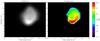 |
Fig. 1 Left: reflectance image of Steins at 2 μm obtained with VIRTIS-M. The X-axis corresponds to the pixels along the slit of the spectrometer, and each line of the Y-axis is relative to the frames (lines) obtained at different times. Right: temperature map retrieved by using only the 104 selected pixels (see the text for more details). |
The exact geometry pointing (latitude and longitude of the 4 pixels’ corners; elevations; emergence, incidence and phase angles; local times) was retrieved using the latest available ephemerides and attitude files reconstructed by the ESA flight dynamics team after the encounter. All spacecraft location and attitude, instrument’s field of view (FOV), and target position in the Rosetta reference frame were used to compute the exact pixel boundaries at the surface of the observed body. We used a shape model developed using the limb method (edge detection of Steins) at the Laboratoire d’Astrophysique de Marseille (Jorda et al., in prep.). Figure 2 shows the computed projected pixels footprints on the shape model in both geometric configurations that correspond to the begining and the end of the observations. Reflected radiance is consistent with the local angles. One can note that pixels located at the limb or very close to it may not be entirely filled by the target, which results in a low level of signal and spectral artifacts.
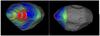 |
Fig. 2 VIRTIS-M cube acquired at closest approach, projected on the shape model of Jorda et al. (in prep.), with orientations corresponding to the beginning (left) and the end (right) of acquisitions (celestial north is at the top). Instrument’s footprints are color-coded in radiance at 1.23 microns. |
2.2. Temperature inversion
All of the VIRTIS cubes were calibrated by means of the instrument transfer function (ITF) developed on the basis of both ground calibration and in-flight data analysis. This function, which is the outcome of the radiometric calibration, allows one to convert from relative units (digital numbers, DN) to physical units of spectral radiance (Wm-2 sr-1 μm-1) accounting for the exposure time and flat-field variations. The VIRTIS-H channel calibration also includes a correction of non-linearity at low signal levels. The I/F ratio is then derived by dividing the spectral radiance by the Kurucz (1997) solar spectrum, convolved to VIRTIS wavelengths and scaled to the Sun distance.
The procedure used here is to fit both the spectral reflectance and the temperature for every spectrum. We use a basic radiance model in which reflectance and near IR emissivity are related through a photometric function, and a single temperature is used for each pixel.
The model is a simplified, atmosphereless version of the one used and described by Erard & Calvin (1997). Radiance at wavelength lambda writes 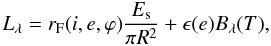 (1)where Bλ is the black body radiance at surface temperature T,
  is the solar irradiance at Steins’s distance, rF and ϵ(e) are the radiance factor and the directional emissivity of the surface at the same wavelength, i is the local incidence angle, e is the local emergence angle, and ϕ is the local phase angle.
In a particular medium of isotropic scatterers, hemispherical emissivity is related to spherical reflectance at each wavelength by Kirchhoff’s law:  (2)The photometric function is here assumed to be Lambertian, which is a reasonable assumption for such a bright material. In the Lambertian approximation, Kirchhoff’s law writes
 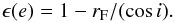 (3)This quantity does not depend on incidence in the Lambertian case. As an alternative, we also used a Lommel-Seeliger model, which normally fits darker materials. In this case, a similar, more complicated formulation of Kirchhoff’s law can be derived. It is used here to estimate the model-dependence of the fit. We stress that the emissivity ϵ used here is derived in the measured near-IR range, therefore at short wavelengths. It may be very different from the long wavelength emissivity ϵIR (in Mid IR), which controls the surface temperature variations (see thermal modeling below).
The retrieved temperatures from VIRTIS-M are ranging up to 225 K, and never exceed 230 K when taking uncertainty measurements into account. VIRTIS’ ability to retrieve temperatures is limited by the cutoff wavelength of its IR focal plane (5.2 μm) as well as by the temperature of its optical parts, so in most cases the instrument cannot sample surface temperatures below ~170 K. The near IR emissivity fitted in the procedure is relatively low (around 0.7 to 0.8, between 1 and 5 μm), and it does not strongly depend on the applied photometric model. These values are expected in the near-IR from modeling (Helbert et al. 2010; Moroz et al. 2006), though they are markedly lower than the values observed in the mid-IR. They are also consistent with the few values published at these wavelengths for minerals (Moroz et al. 2006), and with newer emissivity measurements in laboratory (Maturilli et al. 2010). The overall accuracy on retrieved temperatures is about of 4−5 K.
Because of the spacecraft pointing problem during the C/A phase, VIRTIS-H acquired few data of Steins. However, 20 spectra are found to be entirely located on the disk. They were inverted in a similar way. The retrieved temperatures are in the same range as the temperatures measured by VIRTIS-M, even if the use of those spectra is limited for the thermal inertia retrieving because of the low amount of longitudinal coverage at the surface of the asteroid.
2.3. Pixels selection
The temperature inversion was performed for all of the 209 spectra on the target. Pixels near the limb were filtered out afterward and the variability was studied from the selected spectra only. We filtered the limb by using the signal itself and the consistency between the temperatures derived between two different frames to check the pointing. The parameter is the strength of the signal derivative at 1.5 μm, which is a typical artifact occurring when the FOV is not entirely filled. We also removed pixels with retrieved temperatures lower than 170 K, that may correspond to partially filled pixels or to high contrast temperatures inside the FOV. This provides 104 pixels (i.e., half of the initial selection), spread over 13 different frames, with the field of view entirely filled by the target. Figure 1 (right) represents the map of temperatures. The last three frames (at the top of the map) were obtained very close to the morning terminator.
Figure 3 represents a histogram of the measured temperatures. The surface temperature ranges from 186 to 225 K, with an average value of 204 K. In comparison, the sub-solar temperature for a zero-thermal inertia (i.e., instantaneous re-emission of absorbed flux) is Tss = ((1 − Av)F/(ϵIRσ))1/4, where ϵIR is the mid-IR emissivity and σ is the Stefan constant. With an albedo Av = 0.22 (Keller et al. 2010) and ϵIR ~ 0.9, we expect Tss = 260 K, which is much higher than the maximum observed temperature. This could be explained by a sufficiently significant thermal inertia that weakens the thermal contrast at the surface, and also by deviations from the sub-solar point (noon local time) within the pixels’ field of view.
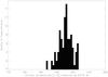 |
Fig. 3 Histogram of the 104 temperature measurements over the 13 selected frames. Minimum and maximum temperatures are 186 and 225 K, respectively. This is lower than the expected sub-solar temperature for an instantaneous thermal equilibrium. |
A strong correlation (with a correlation coefficient r = 0.8) is found between T4 and the reflectance between 1 and 4 μm (Fig. 4). This correlation is much enhanced when limb pixels are filtered out. For a Lambertian surface in instantaneous thermal equilibrium, the temperature is expected to be proportional to cos(incidence)1/4, and the reflectance to be proportional to cos(incidence). Departures from this relationship are expected for non-Lambertian surfaces observed under high emergence and for non-zero thermal inertia. The relationship illustrated in Fig. 4 seems to indicate that the surface is actually almost Lambertian. Furthermore, while thermal inertia seems to be greater than zero, it must be sufficiently low (as compared to rocky-like surfaces) to allow a fast adjustment of the surface temperature.
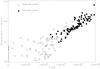 |
Fig. 4 Radiance at 2 μm versus T4. Filled circles correspond to temperatures higher than 170 K and where the pixels are completely filled, i.e., the selected measurements. A Lambertian model would suggest a linear relation between data. |
3. Thermal modeling of Steins
The interpretation of thermal infrared data requires both a shape model of the body and a thermal model, which must be able to predict time-dependent variations of surface temperatures as well as sub-surface temperatures. At each point of the surface, the diurnal variations of the incoming solar flux depend on the spin orientation and the spin rate of the asteroid, but also on the topography. The latter may indeed create some shadows and also some additional heating owing to reflected light inside craters or close to a landslide for example.
3.1. Shape model
As we previously said, only 60% of the surface of Steins was spatially resolved by the OSIRIS cameras. A shape model based on a combination of light-curve inversions obtained from Earth and limb detection at different phase angles was first used to compute the pointing of VIRTIS (see above) and also to provide an estimate of the local angles. An accurate new shape model based on photoclinometry was developed by Jorda et al. (in prep.). This model is much more accurate in terms of local inclination of the slopes. This plays an important role in the amount of absorbed solar flux. The overall dimensions measured along the principal axes of inertia are 6.49 × 5.85 × 4.19 km. The initial model is composed of 68 818 facets, with a surface area and a volume equal to 89.7 km2 and 73.4 km3 respectively. We used a re-sampled version of this shape model, composed of 10% of the total amount of initial facets, i.e., 6880 triangular facets. This re-sampling is intended to reduce the processing time without significantly changing the important small-scale variations of the topography (i.e., around craters for example), especially in the observed area. The local illumination conditions can be computed by using the given shape, and the thermal response is computed accordingly.
3.2. Thermal model
For this purpose, a specific thermal model based on the numerical resolution of thermal conduction equations was developed for this work by the VIRTIS team in the Paris Observatory. Table 1 indicates the parameters we used in the thermal model. This thermal model describes the energy balance at the surface of the body between the flux received from the Sun, the flux re-radiated in space, and the heat conduction in the asteroid itself. Here we neglect heat conduction parallel to the surface and we consider that heat transfer is efficient only in the radial direction; in other words, we only take into account heat conduction through depth. This assumption is valid as long as the diurnal skin depth is more shallow than the average size of the facets. Typical surface area of a facet describing the shape model is roughly 100 m2. The thermal skin depth defines the scale at which the heat wave is divided by e and it is defined as  . K is the thermal conductivity [W m-1 K-1 ] , ρ is the bulk density [kg m-3 ] , C is the heat capacity [J kg1 − K-1 ] , and N [rad s-1 ] is the typical frequency of illumination. N can be either associated to the seasonal variations of lighting (owing to the tilt of the axis or to the eccentricity of the orbit), or to the diurnal variations caused by the spin rate ω. Because we do not consider the long-term thermal evolution of Steins, we here neglect the seasonal thermal skin depth, which is much more shallow than the diurnal thermal skin depth. Thus we assume
  . Typical values of ls for asteroids (with ω ~ few hours) are about a few millimeters and the heat wave that penetrates the regolith is only about ten times higher than the value of the skin depth. This is much less than the average size of each facet and thus validates the 1D conduction assumption.
Physical parameters of the thermal model.
We thus treat each facet of the shape model independently from each other. At each time, the surface energy balance of the facet i is given by 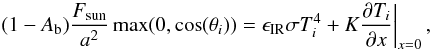 (4)where Ab is the bolometric Bond albedo; Fsun [W m-2 ] the solar flux scaled at 1 AU (i.e., 1373 W m-2); a is the heliocentric distance in AU; ϵIR is the mid-infrared emissivity and differs from the near-IR emissivity derived during the temperature retrieval procedure; σ is the Stefan constant; Ti is the surface temperature of the facet i; K is the thermal conductivity; x is the depth below the surface. The surface level is defined by x = 0. The factor max(0,cos(θi)) is equal to 0 if the facet is not illuminated by the Sun (on the night side) or in the shadow produced by other surrounding facets. In all other cases, it is equal to cos(θi), where θi is the incidence angle of the ith facet at a specific local time. Several authors have published thermal models of asteroids, see e.g., Lagerros (1996, 1998); Spencer (1989); Groussin et al. (2004). They all also used a thermal beaming factor η to include the surface roughness at a sub-pixel scale or the non-zero thermal inertia in the case of disk-unresolved data. Here we neglect the beaming parameter η in a first step, because we later include surface roughness effects (see Sect. 4.2.2).
As the asteroid rotates around its spin axis, the distribution of the incoming sunlight at the surface varies when max(0,cos(θi)) changes over time. Consequently the temperature T varies as a function of time t and depth x. We consider the one-dimensional and time-dependent conductive heat flow equation  (5)This equation is evaluated over the x interval (from 0 at the surface to some depth d). This implicitly assumes that ρ, C, and K do not vary with depth and temperature. Their constancy is a reasonable approximation because the depth considered is pretty small. A more accurate thermal model should later include variations of the density with depth (especially at the first layers), variations of heat capacity and thermal conductivity with temperature, and a sublimation effect that does not play any role for asteroids, but which should be taken into account for comets.
3.2.1. Upper and lower boundary conditions
The boundary condition at the surface of each facet is given by Eq. (4) (x = 0). At the basis of the x interval (i.e. at depth d) there is no heat flux through the boundary: 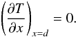 (6)This condition implies that the temperature remains constant below a sufficiently thick layer of depth d. This constant temperature condition is achieved a sufficiently low boundary that is below the diurnal temperature variations, which decay exponentially downward with the characteristic diurnal thermal skin depth ls. We used d = 15ls and checked that integrating to deeper levels does not change the predictions of surface temperatures. Indeed, we found that sub-surface variations of temperature end typically at roughly 5 to 6 skin depths.
3.2.2. Model parameters and numerical solution
The five following parameters have to be constrained: Ab, ϵIR, K, ρ and C. The three last ones, which define the diurnal thermal skin depth of the regolith, can be combined into a single quantity, the so-called thermal inertia  [J K-1 m-2 s−1/2 ] . Because K, C and ρ are assumed to be uniform, the thermal inertia is assumed to be constant whatever the depth is.
Γ is now the only parameter that we will consider when solving the system of Eqs. (4) and (5). The thermal inertia is the physical property that controls both the temperature variations at the surface and the capacity of the subsurface to store energy, given its porosity p.
The mid-IR emissivity ϵIR is assumed to be equal to 0.95, the middle point of the interval 0.9 − 1.0 always quoted in the literature. For the measured temperature (170 − 230 K), the Planck function peaks around 15 μm, so the mid-IR domain corresponds to the wavelength range where the thermal emission is mainly driven by the Planck function itself. Because the emissivity interval 0.9 − 1.0 is very small and the value is near 1.0, the uncertainty on ϵIR has a negligible influence on the calculated thermal flux. ϵIR is also different from the emissivity retrieved in the near infrared when inverting the spectra.
The bolometric Bond albedo, which represents the fraction of absorbed energy integrated over the full spectrum, is taken to be equal to 0.22 as found by Keller et al. (2010). Small deviations from this value will not affect the resulting surface temperature significantly.
For each facet of the shape model, we divided the subsurface structure into 150 identical slabs with an x thickness Δx ~ 0.1ls up to a depth of 15ls and the exact amount of the absorbed solar flux was computed using trajectory and attitude spacecraft files with a time step ΔtFlux = P/200 ~ 108 s (where P is the rotational period). We then extrapolated the amount of absorbed solar flux using a time step ΔtFlux = P/5000, i.e., every 4.3 s. This time step was used for the thermal computation to ensure good convergence of the thermal solution. We used a Cranck-Nicholson algorithm (Crank & Nicholson 1947) to solve the heat equation because this method is unconditionally stable whatever the time and space steps. Moreover, we systematically checked that the Fourier number defined as (KΔ(T))/(ρC(Δx)2) remains lower than 1/2 to avoid oscillations of the solutions (Crank & Nicholson 1947). The different layers were assumed to be at the equilibrium temperature at the beginning of the iterations, and the solution was found for most cases typically after 5 − 6 iterations. To ensure a good convergence, we decided to stop the processing after 10 iterations (i.e., when the algorithm is supposed to have already converged), or when the total absorbed flux is equal to the total emitted flux at the surface within tolerance of 10-4. As a result, we obtained the temperature of each facet versus time over one rotational period.
3.3. Observed infrared flux
To compare the modeled thermal profile with the VIRTIS temperature measurements, we needed to compute to which proportion each facet (k) of the shape model generates the flux measured in the VIRTIS pixels (i,j). In other words, we needed to know the contribution of the facets (k) inside the pixel (i,j), weighted from its projected area. The infrared intensity emitted from each facet (k) is given as  (7)where λ refers to the wavelength, and B(λ,T(k)) is the Planck function computed for the temperature T(k).
We then computed the projection of the VIRTIS-M pixel (i,j) on the shape model and selected all facets that intersect the pixel field of view (Fig. 5). The total infrared flux measured by the VIRTIS-M pixel (i,j) is then defined as  (8)where S(i,j) is Steins’ surface covered by the pixel (i,j), and
  the fractional projected area covered by the facet (k) in the pixel (i,j). The resulting intensity is thus a linear combination of black-bodies weighted by their apparent area as seen from the spacecraft (Fig. 6).
We fitted Iλ,(i,j) by a Planck function weighted by an apparent emissivity called β. The fit was performed for each pixel using an adaptive Levenberg-Marquardt algorithm. β is an indicator of the deviation of Iλ,(i,j) from a perfect black body. When the temperature contrasts are important in the instrument field of view, β can be higher or lower than 1. In most cases, we found that β is very close to unity with an average value of β = 0.985 ± 0.015. Figure 6 (bottom) gives an example of the Iλ,(i,j) deviation from a black body thermal behavior.
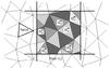 |
Fig. 5 Diagram of facets’ intersection with a pixel (i,j). For a positive detection of an intersection of facets with the pixel (i,j), the fractional area of the considered facets are computed. |
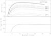 |
Fig. 6 Top: dotted lines represent the Planck functions weighted by the fractional area filled by each facet (with temperature T) that intercepts the pixel (i,j). The solid line is the black body fitted to the sum of dotted lines. Bottom: deviation (in [%]) between the sum of black bodies and the fit. |
We then obtained 104 pixel temperatures for each thermal inertia and for 5000 different time steps.
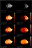 |
Fig. 7 Top: simulated views of Steins obtained at the beginning (left) and at the end (right) of VIRTIS-M observations, i.e., between 18:38:19 and 18:39:22 UTC approximately. The phase angle significantly changed during the observations (see text). In color: simulated thermal maps of Steins for three different thermal inertias (from top to bottom Γ = 10 − 100 − 300 J m-2 K-1 s − 1/2). Surface temperature is color-coded according to the scale on the color bars. The VIRTIS footprints, not represented here, were located on the right side of each image (see Fig. 10). |
4. Thermal properties of Steins
4.1. Thermal maps
We computed both (i) the reflected light assuming a Lommel-Seeliger photometric law (for display purpose) and (ii) the surface temperature using the above thermal model for seven different thermal inertia values (Γ = 0, 10, 25, 50, 75, 100, 150, 200 and 300 J K-1 m-2 s1/2). This was done for the extreme geometries of observations, because the phase angle significantly varies during the closest approach phase where VIRTIS data were successfully acquired. Some results are illustrated in Fig. 7. VIRTIS footprints are not represented in these images for better clarity because they overlap each other and were obtained at different intermediate geometries not shown here. Obviously the shape model we used is only accurate at the observed and illuminated surfaces. The night side of Steins is represented by the simplest convex shape, while the day side is much more accurate than in the previous shape model used in Sect. 2.2. Low thermal inertia implies that surfaces at low incidence angles (e.g., near the sub-solar point) are much warmer (~260 K) than the unlit area, implying a high thermal contrast over the whole surface. In this case, the thermal profile of the regolith roughly follows the reflected light profile because the thermal response occurs almost instantaneously.
When the thermal inertia increases, the surface temperature becomes less heterogeneous. We obtain a sub-solar temperature of 268, 260, 250, 241, 232, 222, 219, and 212 K for a thermal inertia of 0, 10, 25, 50, 75, 100, 150, 200, and 300 J K-1 m-2 s1/2 respectively. Because VIRTIS observed a maximum temperature of 225 K, we can already exclude thermal inertia greater than almost 200 J K-1 m-2 s1/2 when no roughness is assumed. The low boundary of the thermal inertia can be best constrained observing the rate of heating or cooling of the regolith before and after noon local time respectively.
4.2. Comparison with VIRTIS temperature profiles and discussions
We now focus on a direct facet-to-pixel comparison between the output of the model convolved by the VIRTIS footprint and the real data.
4.2.1. Thermal inertia without roughness
We computed the expected modeled temperature in each pixel using Eq. (8) for a set of 12 different thermal inertias. Here we assume that the facets described by the shape model are flat (i.e., no sub-facet scale surface roughness has been added). For each thermal inertia, we obtained 104 values of T that we compared with the data. Very low thermal inertia means that only a small fraction of the solar energy penetrates deeply into the body and that the thermal lag of the surface is short with almost instantaneous adaptation to insolation (thermal equilibrium). We observed that the latter case implies a temperature distribution that is too large (Fig. 8), which is inconsistent with the data. The more Γ increases, the narrower is the temperature distribution. The observed thermal contrast ΔT in the field of view is an indicator of the thermal inertia. It is shown in Fig. 8 (filled region) and compared to the expected theoretical extremes temperatures observed in the field of view and for 12 different thermal inertias. As expected, the maximum temperature that could be observed by VIRTIS decreases when the thermal inertia increases as the central local time of the probed area gets closer to noon. Still for this reason, locations where T reaches its minimum value (which corresponds to craters of depressions where the sun is low above the local horizon), follow the same thermal behavior. According to Fig. 8, the thermal inertia is most probably in the range of 100 − 150 J m-2 K-1 s − 1/2, i.e., almost the value found by Lamy et al. (2008).
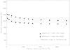 |
Fig. 8 Thermal contrast detectable inside the VIRTIS field of view as a function of thermal inertia when no roughness is assumed. The filled region represents the minimum and maximum temperatures observed by VIRTIS, while the up and down triangles are the expected maximum and minimum observable temperatures for a given thermal inertia Γ respectively. Values of Γ lower than 100 J m-2 K-1 s − 1/2 and higher than 150 J m-2 K-1 s−1/2 are inconsistent with the data. |
We quantitatively compared all temperatures measured in the pixels with the output of the model using a χ2 method to check this result. We found a good match to the data for Γ = 110 J m-2 K-2 s−1/2, confirms the previous estimation. Figure 9 indicates that the value of χ2 significantly increases for lower thermal inertia while values higher than 110 J m-2 K-2 s−1/2 are less constrained. This confirms the result obtained above: very low thermal inertia that is typical of large MBAs (covered by a thick layer of regolith) or of lunar regolith (Delbo’ & Tanga 2009) is clearly rejected for Steins. Furthermore, because we assumed a constant thermal inertia with temperature and depth in our model ( ), we neglected variations of the porosity below the surface, but it may not be constant. This means that Γ may be larger than what we found because the porosity should increase with depth.
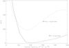 |
Fig. 9 χ2 versus thermal inertia for both cases: with or without rougness. Best results are obtained for Γ = 210 J m-2 K-1 s−1/2 with ξ = 0.2. |
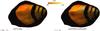 |
Fig. 10 Comparison between Virtis data (left) and the best fit with the roughness model (right) with Γ = 210 J m-2 K-2 s−1/2 and ξ = 0.20. We used 41 290 facets here for a better rendening with high spatial resolution. Warm surface is in yellow, while cold regions appear in dark red. Facets that are included in the selected 104 pixels are color-coded in temperature. North is up. The morning side appears in the middle while noon local time is on the right. |
4.2.2. Thermal inertia with roughness
During the fit procedure we noticed that temperatures measured near the terminator on the morning side (i.e., at the end of observations) are underestimated by the model. This area corresponds to facets that have been less illuminated by the Sun than the ones observed at the begining of observations. The latter ones correspond to the afternoon side being visible.
While the temperature on the morning side should slowly increase as the local solar incidence angle increases, the observed temperatures are still quite high in the morning terminator. We can explain this phenomenon in two different ways:
-
Thermal inertia may vary at the surface of Steins. Even though noobvious surface variations have been detected in the visiblewavelengths (Leyrat et al. 2010),we cannot rule out the hypothesis of potential variations ofthermal properties over the first millimeters below the surface.
-
Roughness at small scales (smaller than the facet dimensions) may be present. This surface roughness allows some facets to face the Sun even for local times very different from noon. These facets are then warmer in the local afternoon or morning side and tend to increase the temperature estimate significantly because the infrared flux is proportional to T4. Roughness is often described by a beaming factor η < 1. In this case, the thermal inertia has to be increased to fit the data. This implies less thermal contrast at the surface heated by the Sun and could then explain the underestimation of T in our non-roughness model.
The beaming factor η, used in the literature to take the roughness into account, was previously not applied in our model. While the thermal inertia was explicitly included by means of K, ρ and C, the facets of the shape model were assumed to be flat. Small-scale roughness here refers to the unresolved topography, i.e., at a scale lower than the size of the facets. Each facet may have irregularities at small scales, which we must take into account in the energy balance. Indeed, roughness adds self-heating and mutual shadowing inside each facet. They must be included in the absorbed flux. In other words, facets receive radiations from the Sun, but also from surrounding facets that scatter sunlight and re-radiate their thermal flux.
To illustrate this, roughness below the resolution of the shape model is treated statistically here. Lagerros (1997) has introduced the self-heating parameter ξ, which is defined as the ratio between the power that directly strikes the surface to the total power emitted from the surface, when kept isothermal. ξ compares the true rough surface area (Arough) and the area of the convex hull (Aflat). The apparent energy coming from the surface is proportional to the area of the flat surface Aflat, while the total energy output is proportional to Arough. Thus, 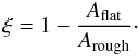 (9)Interestingly, when the self-heating is taken into account, Eq. (4) can be changed to (Davidsson et al. 2009)
  (10)One can note that ξ differs from η in terms of physical meaning because ξ can be directly linked to physical properties. Aflat and Arough can be estimated for a Gaussian distribution function of local slopes. If
  is the mean slope angle of the surface roughness as described by Hapke (1984), then
 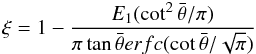 (11)where E1 is the first order exponential integral.
Using visible phase curves obtained by the OSIRIS camera onboard Rosetta during the Steins flyby, Keller et al. (2010) found an average value  ± 3.8 deg with few variations over the observed surface, implying that ξ = 0.20 ± 0.03. This is fairly low and indicates that the small-scale roughness needs to be included in our model, even though it is weak on Steins. Then the effective emissivity ϵIReff included in Eq. (10) is (1 − ϵIRξ)ϵIR = 0.73 ± 0.02. This value is similar to the near infrared emissivity but this is a coincidence because the physical meaning of both of them differs. We emphasize that the ξ value determined with this formalism is mathematically equivalent to η = 1 − (0.9 × 0.2) = 0.82 in the classical formalism often used in the literature. Additionally, ϵIReff is almost similar to the emissivity 0.6 − 0.7 found at 0.53 mm with the microwave instrument MIRO during the flyby.
If we now use the value found for the self-heating parameter to solve the heat conduction, the best fit to the data is obtained for Γ = 210 J m-2 K-2 s − 1/2 with a lower χ2 than the one found without roughness effects (Fig. 9). This shows that a significant degree of roughness is required to reproduce the surface temperature especially for data at high or low incidence angles. However, the few measurements obtained on Steins did not allow us to look for any variation of thermal properties at the surface. Figure 10 shows a comparison between measured and modeled surface temperature (for Γ = 210 J m-2 K-2 s−1/2 and ϵIReff = 0.73) projected on the shape model when roughness is taken into account. Only data corresponding to the selected 104 pixels are shown. The increase of the temperatures depending on the local time is very well reproduced. Areas located at the morning terminator are colder than the ones at local noon in our model. Only the equatorial surge temperature (visible in the model) is fairly detected by VIRTIS, but this is because of the pixel footprint convolution. Figure 9 clearly shows that Γ ≥ 110 J m-2 K-2 s−1/2, with a most likely value of Γ = 210 J m-2 K-2 s−1/2. This confirms a low porosity and the absence of a thick layer of regolith at the surface, as previously found. The degree of microporosity is still difficult to determine when thermal properties are assumed to be constant with depth. A more complex thermal model that treats the heat transfer inside a porous medium is needed for a better interpretation. However, our results are also consistent with Lamy et al. (2008) and add some constraints on the effects of surface roughness.
Interestingly, Gulkis et al. (2010) have shown that a high thermal inertia (in the range 450 − 850 J m-2 K-1 s−1/2) was required to explain variations of VIRTIS temperatures with solar phase. Those results were based on a preliminary data analysis and a simple thermal model with ϵIR = 0.9, but they were inconsistent with the abolute value of temperature measurements. Our analysis based on accurate disk-resolved thermal modeling indicates a lower thermal inertia but are consistent with previous estimations obtained from the Sptizer telescope or from ground (Γ = 150 ± 60 J m-2 K-1 s−1/2 in Lamy et al. 2008).
To put this result into perspective, the Steins surface thermal inertia can be more or less compared to the average value (~200) found for NEA objects (Delbo’ et al. 2007), while thermal inertia of large MBAs is typically lower. Over hundreds of million years of impact processes, MBAs may have developed a fine and thick thermally insulating regolith layer, which is responsible for the low values of their thermal inertia. Kilometer-sized asteroids have collisional lifetimes of only some millions years, and have even less regolith. Consequently they have a larger surface thermal inertia. In addition, the low gravity of these small bodies does not favor ejecta of impacts to fall down on the initial body after the collision.
In the case of Steins, another possibility to explain the relative high thermal inertia is the consequence of the big impact that created the crater near the south pole. It could have ejected a large fraction of the first layers and thus could have exposed the core to space. This less porous material present at the surface may explain why the surface thermal inertia measured by VIRTIS is so high.
4.2.3. Uncertainties
Uncertainties on the estimation of thermal inertia arise from several sources that are difficult to estimate because of the complex procedure described above. Below we summarize the potential sources of errors:
-
1.
The inaccuracy in the instrument pointing and in the shapemodel implies uncertainties in the resulting incidence,emergence, and phase angles. We estimate that this effect impliesabout 10% of errors in the measured radiance. The10%-reduction of resolution in the initial shape model may alsogenerate 2% of additional uncertainty.
-
2.
The uncertainty in the absolute calibration does not play a significant role in the thermal inertia measurement because of its systematical effect on temperatures at all local times.
-
3.
Different assumptions in the method used to retrieve surface temperatures from VIRTIS infrared spectra may lead to uncertainties as high as 4 K where the signal from the target is high enough (namely in the day side of the target and far from its limb). In this case, one source of error may be caused by small features (possibly artifacts) in the spectra at long wavelengths, and can add ~ 5% of error in the thermal inertia.
-
4.
The uncertainty in the albedo (0.22 ± 0.10) implies an uncertainty in the thermal inertia of 2 more percents.
The quadratic sum of all the errors leads to an error of almost 11% in the final thermal inertia. Thus our best estimate is now Γ = 110 ± 13 J m-2 K-1 s − 1/2 when no roughness is assumed, and Γ = 210 ± 30 J m-2 K-1 s − 1/2 with ϵIReff = 0.73 ± 0.02 if we take into account the small-scale roughness (i.e., the most probable case) to describe the surface, with the assumed value of ϵ = 0.9, and the value of ξ = 0.2 derived from the Hapke parameters (OSIRIS images).
5. Conclusions
The Rosetta/VIRTIS instrument has obtained high-quality NIR spectra during the flyby of Steins, allowing a surface temperature inversion. Almost 104 temperature estimates of the disk-resolved have been retrieved at very different phase angles during the closest approach phase. The main results are:
-
1.
Minimum and maximum surface temperatures measured byVIRTIS are 185 Kand 225 K respectively.
-
2.
This thermal contrast is consistent with Γ = 110 ± 13 J m-2 K-1 s − 1/2, assuming a constant thermal inertia of the surface and the absence of small scale roughness.
-
3.
Discrepancies between data and the output of the model at high incidence angles on the morning side near the terminator can be explained by surface roughness at scales smaller than the resolution of the shape model. We showed that when an mid-infrared emissivity of 0.9 is assumed, combined with a small-scale self-heating parameter ξ = 0.2 derived from OSIRIS Hapke parameters describing surface roughness (corresponding to an effective emissivity ϵIReff = 0.73 ± 0.02), the thermal inertia increases to Γ = 210 ± 30 J m-2 K-1 s−1/2. This solution provides a better fit to data. Thus, even if the surface appears relatively smooth, the roughness must be included to interpret and to reproduce thermal data. Variations of the surface temperature with local time are well reproduced by our model.
-
4.
This estimate is larger than previous ground-based or Spitzer estimates, but remains on the same order. Thermal inertia is also consistent with the one found for kilometer-sized near-earth objects. It is still difficult to determine the microporosity when thermal properties are assumed to be constant with depth. For this point, a more complex thermal model that accurately treats the thermal conduction inside a porous medium is needed especially for the comet Churyumov-Gerasimenko, which will be the main target of Rosetta.
The VIRTIS instrument will certainly provide good quality data when the Rosetta spacecraft will reach the Churyumov-Gerasimenko comet in 2014 and will contribute significantly to the monitoing of variations of the surface temperature.
Acknowledgments
We thank Lucas Kamp and Xavier Bonnin for their support in the geometrical computations of VIRTIS data, and Florence Henry for the management of the VIRTIS database in Meudon. We also thank the reviewer for its comments and suggestions, which improved the quality of this work. This work has been supported by the Centre National d’Etudes Spatiales (CNES) and the Agenzia Spaziale Italiana (ASI).
References
- Barucci, M. A., Fulchignoni, M., Fornasier, S., et al. 2005, A&A, 430, 313 [NASA ADS] [CrossRef] [EDP Sciences] [Google Scholar]
- Barucci, M. A., Fulchignoni, M., & Rossi, A. 2007, Space Sci. Rev., 128, 67 [Google Scholar]
- Barucci, M. A., Fornasier, S., Dotto, E., et al. 2008, A&A, 477, 665 [NASA ADS] [CrossRef] [EDP Sciences] [Google Scholar]
- Carvano, J. M., Barucci, M. A., Delbó, M., et al. 2008, A&A, 479, 241 [NASA ADS] [CrossRef] [EDP Sciences] [Google Scholar]
- Clark, B. E., Bus, S. J., Rivkin, A. S., et al. 2004, J. Geophys. Res. (Planets), 109, 2001 [Google Scholar]
- Coradini, A., Capaccioni, F., Drossart, P., et al. 2007, Space Sci. Rev., 128, 529 [NASA ADS] [CrossRef] [Google Scholar]
- Crank, J., & Nicholson, P. 1947, Proc. Camb. Phil. Soc., 43, 50 [Google Scholar]
- Davidsson, B. J. R., Gutiérrez, P. J., & Rickman, H. 2009, Icarus, 201, 335 [NASA ADS] [CrossRef] [Google Scholar]
- Delbo’, M., & Tanga, P. 2009, Planet. Space Sci., 57, 259 [NASA ADS] [CrossRef] [Google Scholar]
- Delbo’, M., Dell’Oro, A., Harris, A. W., Mottola, S., & Mueller, M. 2007, Icarus, 190, 236 [NASA ADS] [CrossRef] [Google Scholar]
- Dotto, E., Perna, D., Fornasier, S., et al. 2009, A&A, 494, L29 [NASA ADS] [CrossRef] [EDP Sciences] [Google Scholar]
- Erard, S., & Calvin, W. 1997, Icarus, 130, 449 [NASA ADS] [CrossRef] [Google Scholar]
- Fornasier, S., Marzari, F., Dotto, E., Barucci, M. A., & Migliorini, A. 2007, A&A, 474, L29 [NASA ADS] [CrossRef] [EDP Sciences] [Google Scholar]
- Fornasier, S., Migliorini, A., Dotto, E., & Barucci, M. A. 2008, Icarus, 196, 119 [NASA ADS] [CrossRef] [Google Scholar]
- Gaffey, M. J., & Kelley, M. S. 2004, in Lunar and Planetary Institute Science Conference Abstracts, ed. S. Mackwell, & E. Stansbery, 35, 1812 [Google Scholar]
- Gaffey, M. J., Reed, K. L., & Kelley, M. S. 1992, Icarus, 100, 95 [NASA ADS] [CrossRef] [Google Scholar]
- Groussin, O., Lamy, P., & Jorda, L. 2004, A&A, 413, 1163 [NASA ADS] [CrossRef] [EDP Sciences] [Google Scholar]
- Gulkis, S., Frerking, M., Crovisier, J., et al. 2007, Space Sci. Rev., 128, 561 [NASA ADS] [CrossRef] [Google Scholar]
- Gulkis, S., Keihm, S., Kamp, L., et al. 2010, Planet. Space Sci., 58, 1077 [NASA ADS] [CrossRef] [Google Scholar]
- Hapke, B. 1984, Icarus, 59, 41 [NASA ADS] [CrossRef] [Google Scholar]
- Helbert, J., Maturilli, A., & D’Amore, M. 2010, in Lunar and Planetary Inst. Technical Report, 41, Lunar and Planetary Institute Science Conference Abstracts, 1502 [Google Scholar]
- Jorda, L., Lamy, P. L., Faury, G., et al. 2008, A&A, 487, 1171 [Google Scholar]
- Jutzi, M., Michel, P., & Benz, W. 2010, A&A, 509, L2 [NASA ADS] [CrossRef] [EDP Sciences] [Google Scholar]
- Keller, H. U., Barbieri, C., Koschny, D., et al. 2010, Science, 327, 190 [NASA ADS] [CrossRef] [PubMed] [Google Scholar]
- Kurucz, R. L. 1997, in The first ISO workshop on Analytical Spectroscopy, ed. A. M. Heras, K. Leech, N. R. Trams, & M. Perry, ESA SP, 419, 193 [Google Scholar]
- Lagerros, J. S. V. 1996, A&A, 315, 625 [NASA ADS] [Google Scholar]
- Lagerros, J. S. V. 1997, A&A, 325, 1226 [NASA ADS] [Google Scholar]
- Lagerros, J. S. V. 1998, A&A, 332, 1123 [NASA ADS] [Google Scholar]
- Lamy, P. L., Jorda, L., Fornasier, S., et al. 2008, A&A, 487, 1187 [NASA ADS] [CrossRef] [EDP Sciences] [Google Scholar]
- Leyrat, C., Fornasier, S., Barucci, A., et al. 2010, Planet. Space Sci., 58, 1097 [Google Scholar]
- Marchi, S., Barbieri, C., Küppers, M., et al. 2010, Planet. Space Sci., 58, 1116 [Google Scholar]
- Maturilli, A., Helbert, J., & D’Amore, M. 2010, AGU Fall Meeting Abstracts, A1509 [Google Scholar]
- Moroz, L., Maturilli, A., & Helbert, J. 2006, in European Planetary Science Congress 2006, 556 [Google Scholar]
- Spencer, J. R. 1989, in Asteroids, Comets, Meteors, ed. C.-I. Lagerkvist, P. Magnusson, & H. Rickman, 121 [Google Scholar]
- Tosi, F., Coradini, A., Capaccioni, F., et al. 2010, Planet. Space Sci., 58, 1066 [NASA ADS] [CrossRef] [Google Scholar]
- Weissman, P. R., Lowry, S. C., & Choi, Y.-J. 2007, A&A, 466, 737 [NASA ADS] [CrossRef] [EDP Sciences] [Google Scholar]
All Tables
All Figures
|
Fig. 1 Left: reflectance image of Steins at 2 μm obtained with VIRTIS-M. The X-axis corresponds to the pixels along the slit of the spectrometer, and each line of the Y-axis is relative to the frames (lines) obtained at different times. Right: temperature map retrieved by using only the 104 selected pixels (see the text for more details). |
| In the text | |
|
Fig. 2 VIRTIS-M cube acquired at closest approach, projected on the shape model of Jorda et al. (in prep.), with orientations corresponding to the beginning (left) and the end (right) of acquisitions (celestial north is at the top). Instrument’s footprints are color-coded in radiance at 1.23 microns. |
| In the text | |
|
Fig. 3 Histogram of the 104 temperature measurements over the 13 selected frames. Minimum and maximum temperatures are 186 and 225 K, respectively. This is lower than the expected sub-solar temperature for an instantaneous thermal equilibrium. |
| In the text | |
|
Fig. 4 Radiance at 2 μm versus T4. Filled circles correspond to temperatures higher than 170 K and where the pixels are completely filled, i.e., the selected measurements. A Lambertian model would suggest a linear relation between data. |
| In the text | |
|
Fig. 5 Diagram of facets’ intersection with a pixel (i,j). For a positive detection of an intersection of facets with the pixel (i,j), the fractional area of the considered facets are computed. |
| In the text | |
|
Fig. 6 Top: dotted lines represent the Planck functions weighted by the fractional area filled by each facet (with temperature T) that intercepts the pixel (i,j). The solid line is the black body fitted to the sum of dotted lines. Bottom: deviation (in [%]) between the sum of black bodies and the fit. |
| In the text | |
|
Fig. 7 Top: simulated views of Steins obtained at the beginning (left) and at the end (right) of VIRTIS-M observations, i.e., between 18:38:19 and 18:39:22 UTC approximately. The phase angle significantly changed during the observations (see text). In color: simulated thermal maps of Steins for three different thermal inertias (from top to bottom Γ = 10 − 100 − 300 J m-2 K-1 s − 1/2). Surface temperature is color-coded according to the scale on the color bars. The VIRTIS footprints, not represented here, were located on the right side of each image (see Fig. 10). |
| In the text | |
|
Fig. 8 Thermal contrast detectable inside the VIRTIS field of view as a function of thermal inertia when no roughness is assumed. The filled region represents the minimum and maximum temperatures observed by VIRTIS, while the up and down triangles are the expected maximum and minimum observable temperatures for a given thermal inertia Γ respectively. Values of Γ lower than 100 J m-2 K-1 s − 1/2 and higher than 150 J m-2 K-1 s−1/2 are inconsistent with the data. |
| In the text | |
|
Fig. 9 χ2 versus thermal inertia for both cases: with or without rougness. Best results are obtained for Γ = 210 J m-2 K-1 s−1/2 with ξ = 0.2. |
| In the text | |
|
Fig. 10 Comparison between Virtis data (left) and the best fit with the roughness model (right) with Γ = 210 J m-2 K-2 s−1/2 and ξ = 0.20. We used 41 290 facets here for a better rendening with high spatial resolution. Warm surface is in yellow, while cold regions appear in dark red. Facets that are included in the selected 104 pixels are color-coded in temperature. North is up. The morning side appears in the middle while noon local time is on the right. |
| In the text | |
Current usage metrics show cumulative count of Article Views (full-text article views including HTML views, PDF and ePub downloads, according to the available data) and Abstracts Views on Vision4Press platform.
Data correspond to usage on the plateform after 2015. The current usage metrics is available 48-96 hours after online publication and is updated daily on week days.
Initial download of the metrics may take a while.