| Issue |
A&A
Volume 530, June 2011
|
|
|---|---|---|
| Article Number | A144 | |
| Number of page(s) | 13 | |
| Section | Galactic structure, stellar clusters and populations | |
| DOI | https://doi.org/10.1051/0004-6361/201116855 | |
| Published online | 26 May 2011 | |
Sulphur abundances in halo giants from the [S ı] line at 1082 nm and the S ı triplet around 1045 nm⋆
1
Department of Astronomy and Theoretical PhysicsLund Observatory, Lund University, Box 43, 221 00 Lund, Sweden
e-mail: This email address is being protected from spambots. You need JavaScript enabled to view it.
2
Department of Physics and Astronomy, Aarhus University, 8000 Aarhus C, Denmark
3
Max Planck Institute for Astrophysics, Karl-Schwarzschild-Strasse 1, Postfach 1317, 857 41 Garching bei München, Germany
4
Department of Physics and Astronomy, Uppsala University, Box 516, 751 20 Uppsala, Sweden
Received: 9 March 2011
Accepted: 5 April 2011
Abstract
Context. It is still debated whether or not the Galactic chemical evolution of sulphur in the halo follows the flat trend with [Fe/H] that is ascribed to the result of explosive nucleosynthesis in type II SNe. It has been suggested that the disagreement between different investigations of sulphur abundances in halo stars might be owing to problems with the diagnostics used, that a new production source of sulphur might be needed in the early Universe, like hypernovae, or that the deposition of supernova ejecta into the interstellar medium is time-delayed.
Aims. The aim of this study is to try to clarify this situation by measuring the sulphur abundance in a sample of halo giants using two diagnostics: the S i triplet around 1045 nm and the [S i] line at 1082 nm. The latter of the two is not believed to be sensitive to non-LTE effects. We can thereby minimize the uncertainties in the diagnostic used and estimate the usefulness of the triplet for the sulphur determination in halo K giants. We will also be able to compare our sulphur abundance differences from the two diagnostics with the expected non-LTE effects in the 1045 nm triplet previously calculated by others.
Methods. High-resolution near-infrared spectra of ten K giants were recorded using the spectrometer CRIRES mounted at VLT. Two standard settings were used, one covering the S i triplet and one covering the [S i] line. The sulphur abundances were individually determined with equivalent widths and synthetic spectra for the two diagnostics using tailored 1D model atmospheres and relying on non-LTE corrections from the litterature. Effects of convective inhomogeneities in the stellar atmospheres are investigated.
Results. The sulphur abundances derived from both the [S i] line and the non-LTE corrected 1045 nm triplet favor a flat trend for the evolution of sulphur. In contrast to some previous studies, we saw no “high” values of [S/Fe] in our sample.
Conclusions. We corroborate the flat trend in the [S/Fe] vs. [Fe/H] plot for halo stars found in some previous studies but do not find a scatter or a rise in [S/Fe] as obtained in other works. We find the sulphur abundances deduced from the non-LTE corrected triplet to be somewhat lower than the abundances from the [S i] line, possibly indicating too large non-LTE corrections. Considering 3D modeling, however, they might instead be too small. Moreover, we show that the [S i] line can be used as a sulphur diagnostic down to [Fe/H] ~ −2.3 in giants.
Key words: Galaxy: evolution / Galaxy: halo / stars: abundances / infrared: stars
Based on observations collected at the European Southern Observatory, Chile (ESO program 080.D-0675(A)).
© ESO, 2011
1. Introduction
Sulphur is an α-element like O, Ne, Mg, Si, Ar, and Ca, and these are believed to be produced mainly in SNe type II by additions of α-particles. The SNe type Ia, on the other hand, mainly produce the iron peak elements Fe, Co, and Ni. Owing to the different life times of the two groups of productions sites, the interstellar medium (ISM) in the early Galaxy is believed to contain a higher abundance of α-elements compared to Fe than later on when the SNe type Ia start expelling iron. Thus, stars that form at a certain time serve as markers of the [α/Fe] 1 ratio in the ISM at that particular stage in the evolution of the Galaxy. This requires that no extra α-elements nor Fe have been produced in the star and contaminated the photosphere during the star’s life. The theory of nucleosynthesis and stellar structure and evolution suggests this to be the case. Because the iron abundance, [Fe/H] , roughly increases with time, an [α/Fe] vs. [Fe/H] plot is expected to show a plateau for the lowest metallicities and a negative slope from the time when the SNe type Ia start producing large amounts of iron. Sulphur in particular, is believed to be produced via oxygen burning just like Si and Ca, and therefore these three elements are expected to vary in lock-step with each other. The expected flat behavior in the [α/Fe] vs. [Fe/H] plot is not unambiguously observed for sulphur in all previous works, however, and hence there is no agreement regarding its evolution. This mismatch with the rest of the α-elements makes the behavior of sulphur interesting to investigate for its own sake, but the Galactic evolution of sulphur is also important to determine for at least two other reasons:
-
the Galactic evolution of sulphur can be matched against the predictions from modeling of supernovae yields and thereby test these models;
-
the volatile properties of sulphur mean that the gas abundances of sulphur measured in, for example, damped Lyman α-systems, which are believed to be galaxies in making, do not need to be corrected for dust depletion to estimate the sulphur abundance in the system. This abundance together with Zn might be used as a proxy for the [α/Fe] and thereby the timescale of the star-formation history of the system can be inferred (Nissen et al. 2004). In order to make these conclusions possible, the Galactic evolution of sulphur needs to be determined first.
It turns out that different works using different sulphur diagnostics have led to several different scenarios for the Galactic evolution of sulphur. From measurements of the 869 nm S i doublet Israelian & Rebolo (2001) and Takada-Hidai et al. (2002) found a negative slope in the [S/Fe] vs. [Fe/H] plot for all observed iron abundances (− 3 ≤ [Fe/H] ≤ + 0.5). To explain this, they proposed either a scenario for sulphur production that involves hypernovae (e.g., Nakamura et al. 2001) or time-delayed iron deposition into the ISM as compared to sulphur (see Ramaty et al. 2000, for a description of the mechanism in connection to [O/Fe] vs. [Fe/H] ). A majority of the stars observed by Israelian & Rebolo (2001) and Takada-Hidai et al. (2002) were later re-analyzed using the roughly ten times stronger S i triplet around 923 nm (Ryde & Lambert 2004; Korn & Ryde 2005), which allowed a more precise abundance determination for metal-poor stars. These new results, contradicting the earlier findings, suggest an evolution analogous to the rest of the α-elements. Neither diagnostic is optimal, however; the 923 nm triplet is stronger than the 869 nm doublet, but it is situated in a spectral region heavily plagued with telluric lines and the middle line of the triplet is situated in the wing of the strong Paschen ζ line.
Takada-Hidai et al. (2005) analyzed 22 stars using both the 923 nm triplet and the 869 nm doublet and found a flat trend from both diagnostics, but significant differences in abundances for the stars with [Fe/H] ≤ − 1.5. These differences might be owing to non-LTE effects in the diagnostics used, which was investigated by Takeda et al. (2005) by calculating non-LTE corrections for the 869 nm doublet, the 923 nm triplet, and in addition the 1045 nm triplet. They used data for determining the evolution of sulphur from Israelian & Rebolo (2001), Takada-Hidai et al. (2002), Ryde & Lambert (2004), Nissen et al. (2004), Takada-Hidai et al. (2005), and some older works and applied their non-LTE corrections to the 869 nm doublet and the 923 nm triplet (the 1045 nm triplet not being observed at the time). Surprisingly, they found that the discrepancies between the evolution of sulphur measured using the different diagnostics increased; the 869 nm doublet suggesting a steady increase of [S/Fe] for lower [Fe/H] and the 923 nm triplet indicating a plateau for halo stars. To resolve this mismatch and check their non-LTE modeling, they proposed observations of the 1045 nm triplet.
Caffau et al. (2005) combined spectra from four observation runs initially aimed at studying other elements into the largest sample of Galactic sulphur abundance measurements with a total of 74 dwarfs. They used the NTT and VLT telescopes, and because the wavelength coverage of the observation runs varied, they did not use the same diagnostics in all their sulphur abundance determinations. For each star they used as many diagnostics as possible of a very weak multiplet around 675 nm, the doublet around 869 nm, and the triplet around 923 nm. They found an [S/Fe] vs. [Fe/H] plot with a large scatter in [S/Fe] for − 2.4 ≤ [Fe/H] ≤ − 1 resembling a combination of the two types of evolution previously described.
The development of better infrared spectrometers has rendered more sulphur lines measurable and the problem with finding a suitable diagnostic for determining sulphur abundance is nowadays less severe. One example is the [S i] line at 1082 nm used in this work. This line is not believed to be affected by non-LTE effects, but unfortunately the [S i] line is undetectable in halo dwarfs for low [Fe/H] . It is detectable in giants down to [Fe/H] ~ −2.5, though. Another example is the triplet around 1045 nm also used in this work. This triplet is not as strong as the triplet at 923 nm, but it is situated in a spectral region almost unaffected by telluric lines. Caffau et al. (2007) investigated the possibility of using the 1045 nm triplet for sulphur determination in disk dwarfs, and it was recently used by them for determining sulphur abundances in four halo dwarfs, corroborating the scatter in [S/Fe] for [Fe/H] ~ −1 found in Caffau et al. (2005) but at a lower level (Caffau et al. 2010).
Takeda & Takada-Hidai (2011) also recently used the 1045 nm triplet to determine [S/Fe] in 33 halo/disk stars, proposing yet a new scenario for the evolution of sulphur: a zig-zag trend with a local plateau around [S/Fe] ~ 0.3 for −2.5 ≤ [Fe/H] ≤ −1.5 preceded by a rise in [S/Fe] for lower [Fe/H] . But this is not confirmed by Spite et al. (2011), who use the 923 nm triplet to determine sulphur abundance in 33 giants and turnoff stars with iron abundances [Fe/H] ≤ −2.5 without finding any stars with “high” [S/Fe] .
Obviously, there is no consensus on the Galactic chemical evolution of sulphur. Is there a scatter or some kind of rise for halo stars or not? In this work we will present and compare sulphur abundance measurements for 10 halo K giants using both the [S i] line at 1082 nm and the 1045 nm triplet. Because the [S i] line is not affected by non-LTE effects, we will also be able to estimate the non-LTE effects of the 1045 nm triplet by comparing the derived sulphur abundances from the two diagnostics. Thereby we will be able to check the validity of the non-LTE corrections calculated by Takeda et al. (2005) for halo K giants. Because non-LTE corrections seem to be significant for most sulphur diagnostics, this empirical test of the corrections is important.
2. Observations
We have observed ten K giants in the Galactic halo using the spectrometer CRIRES (Käufl et al. 2004; Moorwood 2005; Käufl et al. 2006) mounted on VLT. Giants were chosen because the 1082 nm [S i] line is too weak to be observed in metal-poor dwarfs (see Sect. 2.1). CRIRES is a high-resolution echelle spectrometer designed for near-infrared observations, and it uses nodding and jittering to eliminate the sky background and adaptive optics to enhance the S/N. Basic data for the observed stars are shown in Table 1 and a summary of the observations is given in Table 2. The difference in S/N in the two settings is in some cases caused by different integration times and by changes from clouds in the star’s visibility between the two observations.
Basic data for the observed stars.
Summary of the observations with CRIRES/VLT.
The observations were made with a slit width of 0.25′′, resulting in a spectral resolution of R = λ/Δλ ~ 80 000 and 2.5 pixels per resolution element. They were carried out in service mode during October 2007–February 2008. We used two standard settings: one covering the S i triplet around 1045 nm and one covering the [S i] line at 1082 nm. The spectral range of the two settings used are roughly 12 nm with the sulphur lines as centered as possible.
A couple of fast rotating B stars were also observed to check that no telluric lines affect the analyzed lines.
2.1. Blending lines and stellar sample
Using only a few lines, or even just one, for an abundance determination such as ours calls for a particularly careful examination of blends, and if these are found: to try to choose the stellar sample in such a way that the effects of the blending are minimized. For example the [O i] line at 630 nm, analogous to our [S i] line, is blended with a Ni i line, but the blending is not relevant for metal-poor stars (Allende Prieto et al. 2001). To determine for which of our sulphur lines there might be significant blends, we calculated synthetic equivalent widths for all lines in the relevant wavelength region in a grid of 288 model atmospheres. For metals we used a line list of a relevant wavelength section from the VALD I database (Kupka et al. 1999) updated according to Gustafsson et al. (2008). The lists of molecules we were given by Bengt Edvardsson (private communication), which were in turn mostly compiled by Bertrand Plez, and they include CH (Jørgensen et al. 1996), OH (Goldman et al. 1998), CrH (Burrows et al. 2002), SiH (electronic Kurucz2), FeH (Dulick et al. 2003), H2O (Barber et al. 2006), C2 (Querci et al. 1971, 1974), CaH, CN, TiO, VO, and, ZrO (electronic and unpublished Plez3). The list of lines with equivalent widths greater than zero within ± 0.05 nm (Δv ~ 30 km s-1) from the used sulphur lines is presented in Table 3. The equivalent widths of the 1082 nm [S i], the 1045.5 nm and 1045.7 nm triplet lines, and blends with strengths in parity with the relevant sulphur line are shown in Figs. 1–3. The 1045.9 nm triplet line does not have any known significant blends.
Potential blending lines that appear in our grid of models.
The only blend for the [S i] line present in halo giants is that of Cr i, but this line is sufficiently separated from the sulphur line to be resolvable in our high-resolution spectra, see for example the Cr i line in Fig. 5. For the 1045.5 nm and 1045.7 nm S i triplet lines the 1045.54 nm and 1045.69 nm Fe i lines shown in Figs. 2 and 3 are close enough to the relevant sulphur line that they would be indistinguishable.
Our sample stars all have stellar parameters available in the literature (Teff, log g, [Fe/H], and ξmicro). They are chosen to be cool giants to maximize the strength of the [S i] line. Because we are interested in halo stars with [Fe/H] ≤ − 1, the unresolvable Fe i blends expected to most seriously affect the 1045 nm sulphur lines are small compared to the relevant sulphur lines and can safely be ignored. Our lines can thus be considered to be blend free and the measured equivalent widths are those of the sulphur lines only.
Note that as can be seen in Figs. 1–3, one should use these sulphur lines with caution for certain stellar parameters; e.g., for a solar-metallicity dwarf with a temperature of 4500 K the strength of the blending Fe i line would be roughly equal to that of the 1045.5 nm S i triplet line. Moreover, the neighboring Cr i and [S i] lines might become unresolvable and therefore blend when observing at lower resolution.
2.2. Reduction of the spectra
The data were originally reduced using the CRIRES pipeline version 1.5.04. The pipeline makes use of and automatically handles dark frames, flat fields from a halogen lamp, and observations of a ThAr lamp for wavelength calibration. To subtract the sky background, the telescope was nodded between two positions along the slit during the observations. The two frames are subtracted from each other, producing two stellar spectra in vertically different places on the detector arrays. The pixels are subsequently added column wise in the slit direction and extracted for each spectrum exposure by the pipeline and then added to produce the final spectrum of the star.
Unfortunately, there is an optical ghost5 in certain settings of the spectrometer, clearly visible as broad vertical bands in our flat fields (see Figs. 4a and b), but also as smaller dots in our science frames (see Fig. 4c, where a smaller version of the ghost shown in Fig. 4a can be seen). The optical ghost is present in some higher order settings for the echelle grating and is a result of retro-reflection from the detector to the grating, which is redirected onto the detector in a different order.
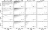 |
Fig. 1 Equivalent widths of the 1082 nm [S i] line and potential blends for different stellar parameters. WCN shows the sum of the three CN lines listed in Table 3. The filled contours mark steps of 10 mÅ and the dotted contours mark the steps of 5 mÅ in between. |
The ghosts in the flat fields lie in such a location on the detector that it will affect one of the two nod positions (compare the flat fields in Figs. 4a and b with the stellar spectra in Fig. 4c). This results in a spectral artifact in the two spectral settings, which most severely affects our analysis of the [S i] line; by chance the spectral artifact lies right on top of the [S i] line in the pipeline reduced spectra, making it impossible to measure (see Fig. 4d). Therefore the data that cover the [S i] line had to be re-reduced. We did this with the CRIRES pipeline version 1.11.06, using the flat field from the triplet setting instead, which was taken close in time. The spectral feature from the ghost is then situated in another part of the spectra that does not affect our analysis (see Fig. 4e). We found that this way of rescuing the data was better than removing the ghost feature by dividing by a telluric star or by reducing the spectra without flat fields, which would not introduce the ghost at all, and then dividing the spectra with a B star to remove the “pixel-to-pixel” variations in the detector. The latter method was used successfully by Nissen et al. (2007) when analysing science-verification spectra from CRIRES without flat fields. Our measured S/N values (per pixel of the spectra) of the reduced spectra reveal that our method indeed produces satisfactory signal-to-noise, as shown in Table 2.
The most relevant parts of the reduced spectra can be seen in Fig. 5. We normalized the spectra and fitted the continua with the IRAF7 task continuum (Tody 1993).
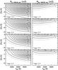 |
Fig. 2 Equivalent widths of the 1045.5 nm S i triplet line and its potential blends for different stellar parameters. The filled contours mark steps of 10 mÅ and the dotted contours mark the steps of 5 mÅ in between. |
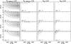 |
Fig. 3 Equivalent widths of the 1045.7 nm S i triplet line and its potential blends for different stellar parameters. WFeH and WCrH show the sum of the three FeH lines and the two CrH lines listed in Table 3. The filled contours mark steps of 10 mÅ and the dotted contours mark the steps of 5 mÅ in between. |
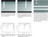 |
Fig. 4 The optical ghost of CRIRES and its effects on reduced spectra. |
2.3. Equivalent widths
The equivalent widths of the 1045 nm S i triplet and the 1082 nm [S i] line were measured with the splot task in IRAF by fitting a Gaussian profile to the line, or, in some cases, by straight numerical integration. For two stars (HD 26297 and HD 29574) the equivalent widths for the forbidden line were measured by de-blending from the neighboring telluric line. The measured values are listed in Table 4. Because our spectra have high S/N, the uncertainties in the measured equivalent widths are mainly caused by uncertainties in the continuum setting. The quoted uncertainties have been estimated by fitting the continuum to achieve a maximum and minimum possible value for the equivalent width. The uncertainties in the measured equivalent widths will in the end produce uncertainties in the [S/Fe] that are less than the uncertainties introduced by uncertainties in the stellar parameters (see Sect. 3.2).
Measured equivalent widths for the observed sulphur lines.
3. Analysis
We have constructed stellar atmosphere models in spherical geometry for the observed stars using the MARCS code (Gustafsson et al. 2008) and the stellar parameters quoted in Table 6. In all models we used an [α/Fe] value of +0.4. The MARCS code computes hydrostatic model photospheres under the assumption of LTE (Local Thermodynamic Equilibrium), chemical equilibrium, homogeneity and the conservation of the total flux. We used these models and the Uppsala Eqwi code (ver. 7.06) together with our measured equivalent widths (see Sect. 2.3) to find two sulphur abundances for every star; one mean value based on the S i 1045 nm triplet and one based on the [S i] 1082 nm line. The observed and synthetic spectra with sulphur abundances determined in the way described can be seen in Fig. 5. The synthetic spectra are calculated with the Bsyn code (ver. 7.09), which is based on the same routines as the MARCS code. The continuous opacities are taken from the model atmospheres. Subsequently, the spectra were broadened by convolving with a rad-tan function with a FWHM given in Table 6 to fit the data, taking into account the macroturbulence of the stellar atmosphere and instrumental broadening.
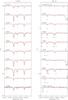 |
Fig. 5 The observed spectra in black and synthetic spectra based on the equivalent width analysis in red. The normalized spectra are shifted by multiples of 0.2 along the flux-axis in the figure. The downward spikes that sometimes occur, e.g. close to the Fe line in HD 83212, are caused by bad pixels. |
3.1. Atomic data
The atomic data for the line list used in the model calculations are taken from the VALD database (Kupka et al. 1999), except for the data for the S i triplet and [S i] line, which were taken from other sources, see Table 5. The [S i] line is an M1 intercombination transition between the triplet ground state and the first excited singlet state. The 1045 nm triplet is three relatively highly exited transitions in the triplet system.
Atomic data for the relevant sulphur transitions.
Adopted stellar parameters for the observed stars.
We note that the log (gf)-value of the [S i] line is debated (Asplund et al. 2009; Caffau et al. 2011), and the derived [S/Fe] values would typically be 0.08 dex lower using the older log (gf)-value used in Caffau et al. (2011) (they use log (gf) = −8.617).
3.2. Stellar parameters
The observed stars all have Hipparcos parallaxes, but unfortunately the uncertainties for most of our observed stars are very large, see Table 1. This in combination with the narrow wavelength coverage of CRIRES makes it impossible to determine the stellar parameters based on our observations alone, so we are forced to use stellar parameters from the literature. The stellar parameters were taken from Fulbright & Johnson (2003), Gratton et al. (2000), and Burris et al. (2000) (in turn mostly taken from Pilachowski et al. 1996) and if a star is listed in two or more of those references the most recent is chosen.
Fulbright & Johnson (2003) obtained Teff from colors, [Fe/H] from Fe ii lines, ξmicro from forcing all Fe i line strengths to give the same iron abundance, and log g from the standard formula: 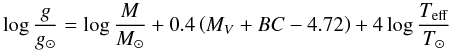 (1)determining absolute magnitudes from literature values (Hanson et al. 1998; Anthony-Twarog & Twarog 1994) in combination with fitting to a 12 Gyr isochrone and, where applicable, by using Hipparcos parallaxes. Gratton et al. (2000) determined Teff from colors, log g from the standard formula (Eq. (1)) with absolute magnitudes from Anthony-Twarog & Twarog (1994), ξmicro from elimination of any trend for abundances as derived from Fe i lines with different strengths, and [Fe/H] from Fe i and Fe ii lines. Burris et al. (2000) determined [Fe/H] from Fe ii lines, but took the rest of the parameters from Pilachowski et al. (1996), who obtained Teff from colors, ξmicro from an iterative process fitting iron and calcium lines, and log g from three independent measurements: the standard formula (Eq. (1)) with absolute magnitudes from the Strömgren c1-index, by assuming that the star’s position in the M92 color–magnitude diagram, and through a derived average relation between surface gravity and effective temperature for metal-poor giants. The adopted stellar parameters are listed in Table 6, where we also give the uncertainties from the references. We note the slight inconsistency in adopting [Fe/H]-values as determined by plane-paralell model photospheres while we use spherical models.
In our observed wavelength region there are four Fe i-lines that we used to check the [Fe/H]-values, given the other three parameters from the references are correct. Our [Fe/H]-values indeed fall within the uncertainties stated in the references. As can be seen in Fig. 5, the Fe and Cr lines in the vicinity of the [S i] line do not fit well with the given parameters for the two stars HD 26297 and HD 29574. Changing the Teff and [Fe/H] within the uncertainty stated in Fulbright & Johnson (2003) will make them fit, though. Despite this mismatch we chose to use the parameters determined by Fulbright & Johnson (2003) because their analysis is based on more and better known iron lines.
Typical uncertainties for the derived sulphur abundances owing to typical uncertainties in the stellar parameters used are listed in Table 7. Obviously the 1045 nm triplet is most sensitive to the temperature, whereas the [S i] line, coming from a transition within the ground configuration, is not affected as much by uncertainties in the effective temperature, but more by uncertainties in the surface gravity through the dependence of the H− bound-free opacity on electron pressure, and the iron abundance. All measured sulphur lines are weak and therefore not much affected by the microturbulence.
A representative example (HD 23798) of the effects on the sulphur abundances owing to uncertainties in the stellar parameters.
3.3. Non-LTE effects
According to Takeda et al. (2005), the non-LTE corrections for the 1045 nm triplet are large and negative, i.e., the LTE abundances should be diminished to correct for the effects. Takeda and collaborators have calculated non-LTE corrections for a grid of model atmospheres with Teff = 4500,5000,5500,6000,6500,7000 K, log g = 1.0,2.0,3.0,4.0, 5.0, and [Fe/H] = −4.0, − 3.0, − 2.0, − 1.0, − 0.5, 0.0, + 0.5. Their calculations use hydrogen collision cross sections based on the classical formula by Drawin (1968, 1969) in the version of Steenbock & Holweger (1984) i.e., SH = 1 is assumed. The work of Takeda et al. (2005) has, to our knowledge, the only available non-LTE corrections for the 1045 nm triplet. However, Korotin (2009) has also performed non-LTE calculations for sulphur, but for the multiplet around 675 nm, the 869 nm doublet, and the 923 nm triplet. The overlapping parts of the two works agree well for lower-temperature stars, but differ for temperatures above 6000 K.
The non-LTE correction used (Takeda et al. 2005) for our observed stars is shown in Table 9. Note that we did not attempt to interpolate in the grid, but chose the corrections from the models best applicable to the stars in this study. We note the slight inconsistency of using spherical model photospheres for our giants while applying non-LTE corrections calculated in plane-parallel geometry. Additional investigations on the effects of non-LTE corrections caused by plane-parallel vs. spherical geometries would be useful.
Because the 1082 nm [S i] line is an inter-combination resonance line, LTE is expected to be a good approximation, because the populations of the energy levels are determined by collisions rather than radiative transitions.
3.4. 3D modeling
We used the set of 3D hydrodynamic model atmospheres of red giants by Collet et al. (2007, 2009) to perform spectral line formation calculations for the [S i] line and the triplet. These calculations were compared to analogous 1D calculations based on MARCS models to estimate the 3D − 1D LTE corrections to the sulphur abundance for giants with different stellar parameters to check the effects of our neglect of convective inhomogeneities on our abundance values. The results are shown in Table 8.
3D–1D corrections for log ϵ(S).
The parameters of the 3D models are not exactly the same as those of our sample stars, but provide a rough estimate of the 3D–1D differences and some qualitative conclusions can be drawn: the corrections for the [S i] line seem to grow larger for higher temperatures, larger surface gravity and lower [Fe/H]. For our sample stars the 3D corrections for the sulphur abundances as derived from the [S i] line all seem to be around or below − 0.1 dex. The corrections for the triplet, on the other hand, are rather constant for the different 3D models and all seem to be around +0.2 dex.
Our 3D analysis for these sulphur lines is the first for giants, but Caffau & Ludwig (2007) explored the 3D correction for the [S i] line in the Sun and Caffau et al. (2007, 2010) explored the 3D corrections for the 1045 nm triplet in the Sun, Procyon, and four other dwarfs. All three works used CO5BOLD 3D hydrodynamical atmospheres for calculating the 3D effects. Caffau & Ludwig (2007) found that the negative 3D-corrections for the [S i] line become more significant (up to roughly − 0.2 dex) for lower [Fe/H] and Caffau et al. (2010) found positive 3D-corrections for the 1045 nm triplet that more or less cancel the non-LTE corrections applied (~ + 0.1 dex). It is of course difficult to compare our models to the models used in Caffau & Ludwig (2007) and Caffau et al. (2007, 2010) because of the large difference in stellar parameters, but it can be noted, however, that all works predict a negative correction for the [S i] line and a positive for the triplet.
We also estimated corrections to the Fe abundances taken from the literature (see Sect. 3.2), and found values from −0.1 dex to −0.2 dex for Fe i and from +0.05 dex to +0.1 dex for Fe ii.
4. Results
4.1. Sulphur
The measured sulphur abundances and the applied non-LTE corrections from Takeda et al. (2005) can be seen in Table 9. In this table we also list the difference between the LTE and non-LTE sulphur abundances derived from the 1045 nm triplet and those derived from the 1082 nm [S i] line. The plot of [S/Fe] vs. [Fe/H] can be seen in Figs. 6 and 7. We used a solar sulphur abundance of log ϵ(S)⊙ = 7.12 (Asplund et al. 2009) and all data in Fig. 6 are put on this scale. A different choice of solar sulphur abundance would simply systematically shift all data by e.g., 0.04 dex using the value of Caffau et al. (2011).
In Table 9 and Figs. 6, 7 we ignored 3D-corrections because we only have a coarse grid of models available for stars with parameters like our stars, but if they were to be applied, they would work in the direction of lowering the sulphur abundances as determined from the [S i] line and adding to the abundances from the 1045 triplet.
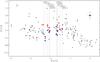 |
Fig. 6 [S/Fe] versus [Fe/H] for the values deduced from the [S i] line shown with red circles and the non-LTE corrected values deduced from the 1045 nm triplet shown with blue squares. Typical uncertainties based on quadratic addition of the values in Table 7 are shown in the upper right hand corner. The plus signs are measurements from Chen et al. (2002), upward pointing triangles from Caffau et al. (2005), asterisks from Caffau et al. (2010), downward pointing triangles from Takeda & Takada-Hidai (2011), and exes from Spite et al. (2011). They are all shifted to log ϵ(S)⊙ = 7.12 (Asplund et al. 2009). |
Derived sulphur abundances.
4.2. Other α-elements
In our narrow wavelength range there are few lines suitable for determining abundances for other α-elements, but there are three Si i lines that can be used. The atomic data are taken from the NIST database and can be seen in Table 10.
Atomic data for the silicon transitions.
Measured equivalent widths for the observed silicon lines.
Derived silicon abundances.
Equivalent widths for the Si i-lines are presented in Table 11. For stars with no values given for the 1037.1 nm and 1084.4 nm lines, no observations were made and for the two stars with no values given for the 1088.3 nm line, the line was covered by a telluric line. The derived silicon abundances are shown in Table 12, and the plot of [Si/Fe] vs. [Fe/H] in Fig. 7. We are not aware of any non-LTE calculations for these Si i-lines.
 |
Fig. 7 [S/Fe] and [Si/Fe] versus [Fe/H]. The left panel shows LTE sulphur abundances deduced from the 1045 nm triplet in black squares and the non-LTE corrected values in red circles. The middle panel shows the sulphur abundances deduced from the 1082 nm [S i] line. The right panel shows the silicon abundance. |
5. Discussion
Until a decade ago, only few studies of sulphur abundances in Galactic halo stars (or, more correctly, for stars more metal-poor than [Fe/H] < − 1), had been made, mainly because of the lack of suitable diagnostic lines. The weak doublet around 869 nm, a transition from a relatively high level at 7.9 eV, was used, but these lines are increasingly difficult to measure as the metallicity decreases. However, their formation is close to LTE conditions, and they are therefore a recommended diagnostic when detectable (Takeda et al. 2005). In 2004 Nissen et al. and Ryde & Lambert used the triplet lines around 923 nm (χexc = 6.5 eV), which are strong enough for determining sulphur abundances at high precision in halo stars, also for the metal-poor ones. The 923 nm triplet is heavily affected by telluric lines, but this can nicely be handled with an observation of a telluric standard star (Ryde & Lambert 2004; Nissen et al. 2004). A severe problem with these stronger lines has been that not all optical CCDs reach up to the wavelengths required. Also, the lines are presumably not formed in LTE (Takeda et al. 2005). Recently, the diagnostic power of new sulphur lines in the near IR, but beyond the reach of normal CCDs, have been explored by means of spectrometers like CRIRES at VLT and near-IR detector arrays (i.e., Ryde 2006; Nissen et al. 2007). These lines are the 1082 nm [S i] line and 1045 nm triplet explored and used in this work. The 1045 nm triplet has non-LTE corrections calculated by Takeda et al. (2005) and the [S i] line, which is a forbidden line, is formed under close to LTE conditions, which is confirmed by non-LTE calculations by Korotin (private communication). This makes analyses based on other sulphur lines than the 869 nm doublet or the 1082 nm [S i] line rely on more or less uncertain8, but necessary, non-LTE calculations.
In this paper we analyzed ten halo giants observed in the near-IR at high spectral resolution to determine the sulphur abundances from the near-IR triplet at 1045 and the forbidden line at 1082 nm. We are able for the first time to analyze the 1082 nm [S i] line for halo stars and show that it is indeed a useful diagnostic in giants down to at least [Fe/H] ~ −2.3. This result agrees with our model predictions (see Fig. 1), showing that it should be usable even for lower [Fe/H] for cool stars with low surface gravity. Our model predictions also show that in dwarfs and subgiants this line is only detectable down to [Fe/H] ~ −1 with the present means.
Our results from the [S i] line favor a flat trend for [S/Fe] as a function of [Fe/H] for halo stars (see Figs. 6 and 7). Fitting a line to the measurements9 gives [S/Fe] = −0.021·[Fe/H] + 0.39 and the simple mean gives [S/Fe] = 0.43 with a standard deviation of σ = 0.11. Because the [S i] line is not believed to be affected by non-LTE effects and 3D effects are smaller, we consider these measurements to be more robust than the measurements using the 1045 nm triplet. By just comparing the two leftmost panels in Fig. 7, it seems that the non-LTE-corrected sulphur abundances from the 1045 nm triplet are similar but perhaps somewhat lower than the abundances from the 1082 nm [S i] line. We conducted a Kolmogorov-Smirnov test10, checking the probability for all our non-LTE corrected [S/Fe] 1045 nm triplet measurements to come from the [S/Fe] distribution as described by our [S i] line measurements. The Kolmogorov-Smirnov statistic for these two distributions is 0.40 and the p-value for this is 0.3111, meaning that formally the two distributions are similar to a low degree and therefore point toward a possible problem with the non-LTE corrections applied to the 1045 nm triplet. When instead comparing the sulphur abundance distribution from the [S i] -line with the LTE sulphur abundance distribution from the triplet, the Kolmogorov-Smirnov statistic is larger as expected: 0.50 and 0.11 for the p-value. Thus the non-LTE corrections of Takeda et al. (2005) at least adjust the LTE distribution of sulphur abundances from the triplet to be more like our resulting abundances from the [S i] -line.
In our analysis we so far ignored 3D-corrections because of the lack of models available for stars with parameters like our stars. It is of course very hard to inter- and extrapolate our coarse 3D-grid to give us information applicable to the observed stars, but it would seem that the positive 3D corrections are large enough (almost +0.2 dex) to cancel the applied non-LTE corrections, making the sulphur abundance measured from the 1045 nm triplet higher than the abundances from the 1082 nm [S i] line. This would make the differences between the two data sets seen in Fig. 7 and in the results of the Kolmogorov-Smirnov test larger again and this might indicate that the non-LTE corrections of Takeda et al. (2005) are too small, or that our estimation of the 3D corrections is too large. From Fig. 6 it indeed seems that the agreement between the two diagnostics would be even better if the [S/Fe] deduced from the [S i] line were lower and the values deduced from the triplet were higher, which at least coincides with the direction of the 3D corrections. It is expected, however, that non-LTE corrections that fully incorporate convective inhomogeneities would be different from our 1D non-LTE corrections. This needs further study where the coupling between 3D and non-LTE are attended to self-consistently. We note that when removing the applied 3D-corrections from Caffau et al.’s (2010) measurements, using the 1045 nm triplet (asterisks in Fig. 6), three of their four values overlap very well with our 1045 nm triplet measurements. This is interesting because the measurements were made with the same instrument, the same diagnostic, and the same non-LTE corrections, but Caffau et al. (2010) used dwarfs instead of giants like we do. This might be another indication that the non-LTE corrections work well in 1D.
Using the [S i] line as a diagnostic for determining sulphur abundance in halo red giants is preferable owing to its small non-LTE and 3D effects, but using only this line is problematic, not only as exemplified by our data where an instrumental ghost unfortunately hit our record of this line, but also because it might be blended by unidentified stellar lines or telluric lines. Fortunately, we could not find any blends and, concerning the ghost, we found a way to rescue the data and determine the sulphur abundance from this line. Because of this risk more lines should be used simultaneously, preferably both the 923 nm and 1045 nm non-LTE corrected triplets. Non-LTE formation of these lines are still not well understood (Takeda et al. 2005). Observing both the 923 nm triplet and the 1082 nm [S i] line would provide the same test of the non-LTE corrections of the 923 nm triplet as presented here for the 1045 nm triplet.
We find that the uncertainties in [S/Fe] in this study will mainly be caused by uncertainties in the stellar parameters (in our case ~ 0.1 dex), the continuum drawing, (in our case < 0.1 dex) and by non-LTE corrections for the triplet as well as effects from convective inhomogeneities. Given these uncertainties, no significant abundance trend in [S/Fe] vs. [Fe/H] but a scatter around [S/Fe] ~ 0.4 can be inferred from our data. To determine whether this scatter is real, we investigated the correlation between [S/Fe]triplet and [S/Fe] [S i] . They would be correlated if the scatter were real, but such a trend would also result from errors in the [Fe/H] used. We cannot find any correlation, but only scatter from what is expected from the uncertainties, except for HD 13979. If we use the newer parameters and iron abundance of Wylie-de Boer et al. (2010) (Teff = 5050 K, log g = 2.25, [Fe/H] = −2.48, ξmicro = 2.35 km s-1), we obtain the sulphur abundances of HD 13979 to more resemble the trend of the others, suggesting that our used [Fe/H] from Burris et al. (2000) might not be correct.
Caffau et al. (2005) find ~ 20% of their analyzed stars to have “high” values of [S/Fe] meaning that our randomly chosen sample of 10 stars would with 90% probability find at least one from this population, if real, but we do not. Concerning the zig-zag trend of Takeda & Takada-Hidai (2011), our sample of stars unfortunately does not go low enough in iron abundance to confirm whether their rise is real or not. Our sample of stars do not have any stars in common with the previous studies to compare abundances from these with our [S i] abundances.
The three Si i lines available in our spectra give a flat silicon abundance trend with roughly equal behavior as the flat sulphur abundance trend in our observed stars, which is what is expected from their common nucleosynthetic origin. The sulphur abundance of HD 13979 is low compared to the others, but the silicon abundance is low as well, meaning that it is possible that this star is low in abundance of α elements, but, as mentioned earlier, the stellar parameters used for this star might not be correct. If we use the newer parameters of Wylie-de Boer et al. (2010), the silicon abundance of HD 13979 also resemble the trend of the others.
As can be seen in Fig. 5, the Fe and Cr lines in the synthetic spectra of HD 26297 and HD 29574 do not fit the data. This is likely owing to the uncertainties in the adopted stellar parameters and the gf-values of the lines. As noted above, we still chose to use the parameters listed in Fulbright & Johnson (2003) because our analysis of [Fe/H] would be based on Fe-lines with lower quality.
An increasing number of investigations, but not all, are gathering evidence toward a view where sulphur follows the abundance trends vs. metallicity in the halo expected for the α elements, i.e., at a constant value to low metallicities. This has implications for models of supernova and hypernova yields and can constrain these models. For example, the hypernova yield models by Nakamura et al. (2001) used by Israelian & Rebolo (2001) to explain their “high” values of [S/Fe] are not confirmed in newer yield calculations by Kobayashi et al. (2006), but they predict a flat [S/Fe] vs. [Fe/H] trend for halo stars in agreement with, e.g., our results. However, the predictions of high [S/Fe] by Nakamura et al. (2001) refer to hypernovae with an explosion energy of 100 × 1051 erg, whereas Kobayashi et al. (2006) only include hypernovae with energies up to 30 × 1051 erg, but it can be noted that Nakamura et al. (2001) also predict enhanced Si/O and Ca/O ratios for the most energetic hypernovae, which are not observed, so it seems that these very energetic hypernovae do not play any role for the chemical evolution above [Fe/H] ~ − 3.
6. Conclusion
In the literature, there are several proposed trends for the evolution of sulphur in the halo phase of the Milky Way. This has implications for our understanding of the nucleosynthesis of sulphur and the sites where this occurs. The three currently discussed trends are the flat trend of e.g., Spite et al. (2011), the scatter trend of Caffau et al. (2010), and the recent zig-zag trend of Takeda & Takada-Hidai (2011).
In trying to minimize the effects of non-LTE in the diagnostic, we used the 1082 nm [S i] line for which LTE is a good approximation and found a flat trend for [S/Fe] similar to that in Spite et al. (2011) and the trends expected for the α-elements. We also determined the sulphur abundance from the 1045 nm triplet to investigate its usefulness in giants, especially concerning its sensitivity to non-LTE. Our empirical differences can be compared with existing non-LTE corrections. We find that with the non-LTE corrections from Takeda et al. (2005) for the 1045 nm triplet, the derived sulphur abundance in most giants are closer to the abundance determined from the forbidden line, but the data hint towards these non-LTE corrections being too large when 1D models are used. They might be too small for 3D, however. This is based on mostly qualitative conclusions from a coarse 3D model grid though, and it might be that the discrepancy between the two data sets is caused by exaggerated 3D effects and not by faulty non-LTE corrections.
Not only because it is formed under LTE conditions, but also because the 3D corrections are smaller for the [S i] line compared to the 1045 nm triplet, the 1082 nm [S i] line would be the preferred diagnostic of the two used in this paper. Even though the two diagnostics do not produce the exact same trend, our sulphur abundance from the near-IR triplet, corrected for the calculated non-LTE effects, also corroborates the idea of sulphur behaving like a normal α-element, and we do not find any “high” values for [S/Fe] like in the scatter trend of Caffau et al. (2010). Neither do we find any “high” values for [S/Fe] like in the zig-zag trend of Takeda & Takada-Hidai (2011), but unfortunately our sample of giants does not go to sufficiently low [Fe/H] to sample the region where their values of [S/Fe] rise.
We demonstrated that both the 1045 nm triplet and the 1082 nm [S i] line should be useful for investigations of the halo phase of the Milky Way. The [S i] line has the advantage of not being subject to uncertain non-LTE corrections, but it also has the drawback of being a single line. An increasing number of investigations point toward sulphur behaving as a traditional α-element in the trends in [α/Fe] vs. [Fe/H] plots. However, there still exist considerable claims for higher values as the metallicity decreases. To convincingly determine the situation for the α- element sulphur, further systematic and homogeneous investigations are needed, using as many diagnostics and with as sophisticated analyses as possible (including non-LTE and 3D modeling).
The notation ![Mathematical equation: \hbox{$[\mathrm{A} / \mathrm{B}]=\log \left( N_{\mathrm{A}} / N_{\mathrm{B}} \right)_{*}-\log \left( N_{\mathrm{A}} / N_{\mathrm{B}} \right)_{\odot}$}](/articles/aa/full_html/2011/06/aa16855-11/aa16855-11-eq201.png) , where NA and NB are the number abundances of elements A and B respectively.
, where NA and NB are the number abundances of elements A and B respectively.
Described in the CRIRES Pipeline User Manual, Issue 1.0 at ftp://ftp.eso.org/pub/dfs/pipelines/crire/crire-pipeline-manual-1.0.pdf
Described in the CRIRES User Manual at http://www.eso.org/sci/facilities/paranal/instruments/crires/doc/
Described in the CRIRES Pipeline User Manual, Issue 1.4 at ftp://ftp.eso.org/pub/dfs/pipelines/crire/crire-pipeline-manual-1.4.pdf
IRAF is distributed by the National Optical Astronomy Observatories, which are operated by the Association of Universities for Research in Astronomy, Inc., under cooperative agreement with the National Science Foundation.
Non-LTE calculations are subject to a number of more or less significant uncertainties and assumptions. The non-LTE corrections are therefore also uncertain.
We used the least-squares linear fit implemented in the routine fitexy presented in NASA’s IDL library at http://idlastro.gsfc.nasa.gov/. The routine takes the uncertainties in both and into account.
We used the routine kstwo from Press et al. (1992).
The Kolmogorov-Smirnov statistic gives the maximum deviation between the cumulative distribution function of the triplet sulphur abundances from the values deduced from the [S i] -line. The p-value takes values between 0 and ,1 giving the significance level of the K-S statistic. A high p-value would in our case show that the cumulative distribution function of our non-LTE corrected [S/Fe] 1045 nm triplet measurements is similar to the cumulative distribution function of our [S/Fe] [S i] line measurements.
Acknowledgments
We would like to thank Sergey Korotin for helpful discussions regarding non-LTE effects. This research has been partly supported by the Royal Physiographic Society in Lund, Stiftelsen Walter Gyllenbergs fond and Märta och Erik Holmbergs donation. Also support from the Swedish Research Council, VR, project number 621-2008-4245, is acknowledged. N.R. is a Royal Swedish Academy of Sciences Research Fellow supported by a grant from the Knut and Alice Wallenberg Foundation. K.E. gratefully acknowledge support
from the Swedish Research Council. This publication made use of the SIMBAD database, operated at CDS, Strasbourg, France and NASA’s Astrophysics Data System.
References
- Allen de Prieto, C., Lambert, D. L., & Asplund, M. 2001, ApJ, 556, L63 [NASA ADS] [CrossRef] [Google Scholar]
- Anthony-Twarog, B. J., & Twarog, B. A. 1994, AJ, 107, 1577 [NASA ADS] [CrossRef] [Google Scholar]
- Asplund, M., Grevesse, N., Sauval, A. J., & Scott, P. 2009, ARA&A, 47, 481 [NASA ADS] [CrossRef] [Google Scholar]
- Barber, R. J., Tennyson, J., Harris, G. J., & Tolchenov, R. N. 2006, MNRAS, 368, 1087 [NASA ADS] [CrossRef] [Google Scholar]
- Burris, D. L., Pilachowski, C. A., Armandroff, T. E., et al. 2000, ApJ, 544, 302 [NASA ADS] [CrossRef] [Google Scholar]
- Burrows, A., Ram, R. S., Bernath, P., Sharp, C. M., & Milsom, J. A. 2002, ApJ, 577, 986 [NASA ADS] [CrossRef] [Google Scholar]
- Caffau, E., & Ludwig, H. 2007, A&A, 467, L11 [NASA ADS] [CrossRef] [EDP Sciences] [Google Scholar]
- Caffau, E., Bonifacio, P., Faraggiana, R., et al. 2005, A&A, 441, 533 [NASA ADS] [CrossRef] [EDP Sciences] [Google Scholar]
- Caffau, E., Faraggiana, R., Bonifacio, P., Ludwig, H., & Steffen, M. 2007, A&A, 470, 699 [NASA ADS] [CrossRef] [EDP Sciences] [Google Scholar]
- Caffau, E., Sbordone, L., Ludwig, H., Bonifacio, P., & Spite, M. 2010, Astron. Nachr., 331, 725 [NASA ADS] [CrossRef] [Google Scholar]
- Caffau, E., Ludwig, H., Steffen, M., Freytag, B., & Bonifacio, P. 2011, Sol. Phys., 268, 255 [NASA ADS] [CrossRef] [Google Scholar]
- Chen, Y. Q., Nissen, P. E., Zhao, G., & Asplund, M. 2002, A&A, 390, 225 [NASA ADS] [CrossRef] [EDP Sciences] [Google Scholar]
- Collet, R., Asplund, M., & Trampedach, R. 2007, A&A, 469, 687 [NASA ADS] [CrossRef] [EDP Sciences] [Google Scholar]
- Collet, R., Nordlund, Å., Asplund, M., Hayek, W., & Trampedach, R. 2009, Mem. Soc. Astron. Ital., 80, 719 [Google Scholar]
- Drawin, H. 1968, Z. Phys., 211, 404 [Google Scholar]
- Drawin, H. W. 1969, Z. Phys., 225, 483 [Google Scholar]
- Dulick, M., Bauschlicher, Jr., C. W., Burrows, A., et al. 2003, ApJ, 594, 651 [NASA ADS] [CrossRef] [Google Scholar]
- Froese Fischer, C., & Tachiev, G. 2011, MCHF/MCDHF Collection, Version 2 [Google Scholar]
- Fulbright, J. P., & Johnson, J. A. 2003, ApJ, 595, 1154 [NASA ADS] [CrossRef] [Google Scholar]
- Goldman, A., Schoenfeld, W. G., Goorvitch, D., et al. 1998, J. Quant. Spec. Radiat. Transf., 59, 453 [Google Scholar]
- Gratton, R. G., Sneden, C., Carretta, E., & Bragaglia, A. 2000, A&A, 354, 169 [NASA ADS] [Google Scholar]
- Gustafsson, B., Edvardsson, B., Eriksson, K., et al. 2008, A&A, 486, 951 [NASA ADS] [CrossRef] [EDP Sciences] [Google Scholar]
- Hanson, R. B., Sneden, C., Kraft, R. P., & Fulbright, J. 1998, AJ, 116, 1286 [NASA ADS] [CrossRef] [Google Scholar]
- Israelian, G., & Rebolo, R. 2001, ApJ, 557, L43 [NASA ADS] [CrossRef] [Google Scholar]
- Jørgensen, U. G., Larsson, M., Iwamae, A., & Yu, B. 1996, A&A, 315, 204 [NASA ADS] [Google Scholar]
- Käufl, H., Ballester, P., Biereichel, P., et al. 2004, in SPIE Conf. Ser., 5492, SPIE Proc., ed. A. F. M. Moorwood, & M. Iye, 1218 [Google Scholar]
- Käufl, H. U., Amico, P., Ballester, P., et al. 2006, The Messenger, 126, 32 [NASA ADS] [Google Scholar]
- Kelleher, D. E., & Podobedova, L. I. 2008, J. Phys. Chem. Ref. Data, 37, 1285 [NASA ADS] [CrossRef] [Google Scholar]
- Kobayashi, C., Umeda, H., Nomoto, K., Tominaga, N., & Ohkubo, T. 2006, ApJ, 653, 1145 [NASA ADS] [CrossRef] [Google Scholar]
- Korn, A. J., & Ryde, N. 2005, A&A, 443, 1029 [NASA ADS] [CrossRef] [EDP Sciences] [Google Scholar]
- Korotin, S. A. 2009, Astron. Rep., 53, 651 [NASA ADS] [CrossRef] [Google Scholar]
- Kupka, F., Piskunov, N., Ryabchikova, T. A., Stempels, H. C., & Weiss, W. W. 1999, A&AS, 138, 119 [NASA ADS] [CrossRef] [EDP Sciences] [MathSciNet] [PubMed] [Google Scholar]
- Moorwood, A. 2005, in High Resolution Infrared Spectroscopy in Astronomy, ed. H. U. Käufl, R. Siebenmorgen, & A. Moorwood, 15 [Google Scholar]
- Nahar, S. N., & Pradhan, A. K. 1993, J. Phys. B, 26, 1109 [NASA ADS] [CrossRef] [Google Scholar]
- Nakamura, T., Umeda, H., Iwamoto, K., et al. 2001, ApJ, 555, 880 [NASA ADS] [CrossRef] [Google Scholar]
- Nissen, P. E., Chen, Y. Q., Asplund, M., & Pettini, M. 2004, A&A, 415, 993 [NASA ADS] [CrossRef] [EDP Sciences] [Google Scholar]
- Nissen, P. E., Akerman, C., Asplund, M., et al. 2007, A&A, 469, 319 [NASA ADS] [CrossRef] [EDP Sciences] [Google Scholar]
- Perryman, M. A. C., Lindegren, L., Kovalevsky, J., et al. 1997, A&A, 323, L49 [NASA ADS] [Google Scholar]
- Pilachowski, C. A., Sneden, C., & Kraft, R. P. 1996, AJ, 111, 1689 [NASA ADS] [CrossRef] [Google Scholar]
- Press, W. H., Teukolsky, S. A., Vetterling, W. T., & Flannery, B. P. 1992, Numerical recipes in C. The art of scientific computing [Google Scholar]
- Querci, F., Querci, M., & Kunde, V. G. 1971, A&A, 15, 256 [NASA ADS] [Google Scholar]
- Querci, F., Querci, M., & Tsuji, T. 1974, A&A, 31, 265 [NASA ADS] [Google Scholar]
- Radziemski, L. J., & Andrew, K. L. 1965, J. Opt. Soc. Am., 55, 474 [NASA ADS] [CrossRef] [Google Scholar]
- Ramaty, R., Scully, S. T., Lingenfelter, R. E., & Kozlovsky, B. 2000, ApJ, 534, 747 [NASA ADS] [CrossRef] [Google Scholar]
- Ryde, N. 2006, A&A, 455, L13 [NASA ADS] [CrossRef] [EDP Sciences] [Google Scholar]
- Ryde, N., & Lambert, D. L. 2004, A&A, 415, 559 [NASA ADS] [CrossRef] [EDP Sciences] [Google Scholar]
- Spite, M., Caffau, E., Andrievsky, S. M., et al. 2011, A&A, 528, A9 [NASA ADS] [CrossRef] [EDP Sciences] [Google Scholar]
- Steenbock, W., & Holweger, H. 1984, A&A, 130, 319 [NASA ADS] [Google Scholar]
- Takada-Hidai, M., Takeda, Y., Sato, S., et al. 2002, ApJ, 573, 614 [NASA ADS] [CrossRef] [Google Scholar]
- Takada-Hidai, M., Saito, Y., Takeda, Y., et al. 2005, PASJ, 57, 347 [NASA ADS] [CrossRef] [Google Scholar]
- Takeda, Y., & Takada-Hidai, M. 2011, PASJ, 63, S537 [NASA ADS] [Google Scholar]
- Takeda, Y., Hashimoto, O., Taguchi, H., et al. 2005, PASJ, 57, 751 [NASA ADS] [Google Scholar]
- Tody, D. 1993, in ASPC, Astronomical Data Analysis Software and Systems II, ed. R. J. Hanisch, R. J. V. Brissenden, & J. Barnes, 52, 173 [Google Scholar]
- Wylie-de Boer, E., Freeman, K., & Williams, M. 2010, AJ, 139, 636 [NASA ADS] [CrossRef] [Google Scholar]
- Zerne, R., Caiyan, L., Berzinsh, U., & Svanberg, S. 1997, Phys. Scr., 56, 459 [NASA ADS] [CrossRef] [Google Scholar]
All Tables
A representative example (HD 23798) of the effects on the sulphur abundances owing to uncertainties in the stellar parameters.
All Figures
|
Fig. 1 Equivalent widths of the 1082 nm [S i] line and potential blends for different stellar parameters. WCN shows the sum of the three CN lines listed in Table 3. The filled contours mark steps of 10 mÅ and the dotted contours mark the steps of 5 mÅ in between. |
| In the text | |
|
Fig. 2 Equivalent widths of the 1045.5 nm S i triplet line and its potential blends for different stellar parameters. The filled contours mark steps of 10 mÅ and the dotted contours mark the steps of 5 mÅ in between. |
| In the text | |
|
Fig. 3 Equivalent widths of the 1045.7 nm S i triplet line and its potential blends for different stellar parameters. WFeH and WCrH show the sum of the three FeH lines and the two CrH lines listed in Table 3. The filled contours mark steps of 10 mÅ and the dotted contours mark the steps of 5 mÅ in between. |
| In the text | |
|
Fig. 4 The optical ghost of CRIRES and its effects on reduced spectra. |
| In the text | |
|
Fig. 5 The observed spectra in black and synthetic spectra based on the equivalent width analysis in red. The normalized spectra are shifted by multiples of 0.2 along the flux-axis in the figure. The downward spikes that sometimes occur, e.g. close to the Fe line in HD 83212, are caused by bad pixels. |
| In the text | |
|
Fig. 6 [S/Fe] versus [Fe/H] for the values deduced from the [S i] line shown with red circles and the non-LTE corrected values deduced from the 1045 nm triplet shown with blue squares. Typical uncertainties based on quadratic addition of the values in Table 7 are shown in the upper right hand corner. The plus signs are measurements from Chen et al. (2002), upward pointing triangles from Caffau et al. (2005), asterisks from Caffau et al. (2010), downward pointing triangles from Takeda & Takada-Hidai (2011), and exes from Spite et al. (2011). They are all shifted to log ϵ(S)⊙ = 7.12 (Asplund et al. 2009). |
| In the text | |
|
Fig. 7 [S/Fe] and [Si/Fe] versus [Fe/H]. The left panel shows LTE sulphur abundances deduced from the 1045 nm triplet in black squares and the non-LTE corrected values in red circles. The middle panel shows the sulphur abundances deduced from the 1082 nm [S i] line. The right panel shows the silicon abundance. |
| In the text | |
Current usage metrics show cumulative count of Article Views (full-text article views including HTML views, PDF and ePub downloads, according to the available data) and Abstracts Views on Vision4Press platform.
Data correspond to usage on the plateform after 2015. The current usage metrics is available 48-96 hours after online publication and is updated daily on week days.
Initial download of the metrics may take a while.