| Issue |
A&A
Volume 530, June 2011
|
|
|---|---|---|
| Article Number | A64 | |
| Number of page(s) | 11 | |
| Section | Interstellar and circumstellar matter | |
| DOI | https://doi.org/10.1051/0004-6361/201016383 | |
| Published online | 11 May 2011 | |
Probing the evolution of molecular cloud structure
II. From chaos to confinement
1
Max-Planck-Institute for Astronomy,
Königstuhl 17,
69117
Heidelberg,
Germany
e-mail: This email address is being protected from spambots. You need JavaScript enabled to view it.
; This email address is being protected from spambots. You need JavaScript enabled to view it.
; This email address is being protected from spambots. You need JavaScript enabled to view it.
2
Zentrum für Astronomie der Universitat Heidelberg, Institut für
Theoretische Astrophysik, 69120
Heidelberg,
Germany
3
Ecole Normale Supérieure de Lyon, CRAL,
69364
Lyon,
France
Received:
21
December
2010
Accepted:
27
March
2011
Abstract
We present an analysis of the large-scale molecular cloud structure and of the stability
of clumpy structures in nearby molecular clouds. In our recent work, we identified a
structural transition in molecular clouds by studying the probability distributions of
their gas column densities. In this paper, we further examine the nature of this
transition. The transition takes place at the visual extinction of
 mag, or
equivalently, at
Σtail ≈ 40−80 M⊙ pc-2. The clumps
identified above this limit have wide ranges of masses and sizes, but a remarkably
constant mean volume density of
mag, or
equivalently, at
Σtail ≈ 40−80 M⊙ pc-2. The clumps
identified above this limit have wide ranges of masses and sizes, but a remarkably
constant mean volume density of  cm-3.
This is 5−10 times higher than the density of the medium surrounding the clumps. By
examining the stability of the clumps, we show that they are gravitationally unbound
entities, and that the external pressure from the parental molecular cloud is a
significant source of confining pressure for them. Then, the structural transition at
cm-3.
This is 5−10 times higher than the density of the medium surrounding the clumps. By
examining the stability of the clumps, we show that they are gravitationally unbound
entities, and that the external pressure from the parental molecular cloud is a
significant source of confining pressure for them. Then, the structural transition at
 may be
linked to a transition between this population and the surrounding medium. The
star-formation rates in the clouds correlate strongly with the total mass in the clumps,
i.e., with the mass above , and drops
abruptly below that threshold. These results imply that the formation of pressure-confined
clumps introduces a prerequisite for star formation. Furthermore, they give a physically
motivated explanation for the recently reported relation between the star-formation rates
and the amount of dense material in molecular clouds. Likewise, they give rise to a
natural threshold for star formation at .
may be
linked to a transition between this population and the surrounding medium. The
star-formation rates in the clouds correlate strongly with the total mass in the clumps,
i.e., with the mass above , and drops
abruptly below that threshold. These results imply that the formation of pressure-confined
clumps introduces a prerequisite for star formation. Furthermore, they give a physically
motivated explanation for the recently reported relation between the star-formation rates
and the amount of dense material in molecular clouds. Likewise, they give rise to a
natural threshold for star formation at .
Key words: ISM: clouds / ISM: structure / stars: formation / dust, extinction / evolution
© ESO, 2011
1. Introduction
Formation of dense, self-gravitating structures inside more diffuse, large-scale molecular clouds is the ultimate prerequisite for star formation. In addition to self-gravitating dense cores, molecular clouds in which star formation is taking place show exhaustive structural complexity characterized by large contrasts in both density and velocity. From the general observation that almost all known molecular clouds harbor young stars, it is known that the formation of structures capable of star formation (or alternatively, cloud dissipation) must proceed relatively rapidly compared to the life-times of molecular clouds. Likely as a result of this complexity and rapid development, molecular clouds also show wide ranges of star-forming efficiencies and -rates (e.g. Heiderman et al. 2010; Lada et al. 2010). This connection between the cloud structure and the capability of a cloud to form stars makes determining the roles of processes and parameters that control the cloud structure a fundamental open topic in the physics of star formation (reviewed, e.g., by McKee & Ostriker 2007; Mac Low & Klessen 2004).
In the current analytic models of star formation, one particularly important structural parameter of molecular clouds is the probability density function (PDF, hereafter) of volume densities, which describes the probability of a volume dV to have a density between [ρ,ρ + dρ]. In these theories, the function has pivotal role: it is used to explain among others the initial mass function of stars and the star formation rates and efficiencies of molecular clouds (e.g. Padoan & Nordlund 2002; Krumholz & McKee 2005; Elmegreen 2008; Hennebelle & Chabrier 2009). In particular, this distribution is expected to take a log-normal shape in isothermal, turbulent media that are not significantly affected by the self-gravity of gas (e.g. Vázquez-Semadeni 1994; Padoan et al. 1997; Ostriker et al. 1999; Federrath et al. 2008b). Most importantly from the observational point-of-view, the log-normality of the distribution is expected to be reflected in the probability distributions of column densities in molecular clouds (Vázquez-Semadeni & García 2001; Goodman et al. 2009; Federrath et al. 2010). Also, a method has recently been developed to attain information of the actual three-dimensional density PDF based on the observed, two-dimensional column density PDFs (Brunt et al. 2010a,b; Brunt 2010). Even though it has been pointed out that the general log-normal-like form for the (column) density PDF can be borne out by various processes (Tassis et al. 2010), it is obvious that a reliable theory of cloud structure must agree with the observed characteristics of the distribution. This is particularly the case if the probability distribution shows any scale-dependent features and/or time evolution. These properties have indeed been predicted, e.g. in the presence of strong self-gravity (Klessen 2000; Federrath et al. 2008a; Cho & Kim 2011; Kritsuk et al. 2011), and scale-dependent features have also recently been observed (Kainulainen et al. 2009b; Froebrich & Rowles 2010; Pineda et al. 2010b). This makes probing the column density probability distributions one parametner of cloud structure that can be used to constrain analytic star formation theories.
However, the connection between theoretical and numerical predictions with observations of the PDF has scarcely been investigated. The studies in which the column density PDFs of mostly individual clouds have been examined have found a qualitative agreement with the predicted log-normal shape (e.g., Ridge et al. 2006b; Goodman et al. 2009; Butler & Tan 2009). The lack of systematic studies of column density PDFs has been mostly due to observational obstacles: all observational tracers of the cloud mass distribution suffer from shortcomings specific to the tracer in question (see, e.g., Goodman et al. 2009). Generally, the dynamical ranges probed by different molecular emission line tracers are often narrow, thereby probing only a limited range of the PDF. Dust continuum emission observations probe a wider dynamical range of column densities, but become insensitive at column densities below N ≲ a few × 1021 cm-2, thus missing a regime where most of the cloud mass is. This is the case also for dust extinction measurements using infrared shadowing features. In addition to these restrictions, mapping nearby cloud complexes that often span several degrees on the sky at high sensitivity requires a colossal observational effort, which is not generally feasible through typical observing campaigns. Dust extinction mapping in the near-infrared reaches only modest column densities of N ≲ a few × 1022 cm-2, thereby mostly missing dense star-forming clumps and cores. However, near-infrared extinction mapping reaches the low column densities N ~ 1−3 × 1022 cm-2 very efficiently (Lombardi & Alves 2001), a regime where most of the cloud mass is. Therefore, it provides a feasible tool to measure the column density PDFs at the scales of entire cloud complexes. Near-infrared extinction mapping has indeed been used for this purpose recently, especially by Kainulainen et al. (2009b; see also Lombardi et al. 2006, 2008b; Froebrich & Rowles 2010; Lombardi et al. 2010; Pineda et al. 2010b).
In our recent work (Kainulainen et al. 2009b, Paper I hereafter), we presented the first systematic study of the column density PDFs in all nearby molecular clouds closer than 200 pc. We used near-infrared dust extinction maps of 23 molecular clouds to identify a transition in the PDF shape from a log-normal-like shape at lower column densities to a power-law-like shape at higher column densities. This transition is characteristic to all star-forming molecular clouds. However, we showed that some of the non-star-forming clouds in our sample did not have the transition, but their PDFs were well fitted by a log-normal over the entire range of column densities above the detection limit. This led us to speculate that the PDF feature is linked to a transition from a quiescent regime dominated by turbulent motions to a regime of active star formation dominated by gravity. The non-star-forming clouds that do not show the feature would then entirely belong to the former regime, and during their subsequent evolution toward star formation, gravitationally dominated structures would appear that would also induce a transition of the shape of their PDFs.
In this paper, we present a more detailed analysis of the structural transition that is identified from the column density PDFs. In particular, we will examine the physical characteristics and stability of the structures that are identified with the PDFs. With this analysis, we will show that the change in the PDF shape can be understood as a transition between the diffuse, interclump medium and a population of clumps that are gravitationally unbound, but are significantly supported against dispersal by the external pressure imposed on them by the surrounding medium. This interpretation links the PDF shape to a physically motivated explanation for the relation between star-formation rates and the amount of high-density material in molecular clouds that was recently reported by Lada et al. (2010), and it also connects it to the threshold of star formation in molecular clouds.
In Sect. 2 we briefly describe the dust column density data used in this paper. In Sect. 3 we characterize the structures identified from the column density maps and examine their stability. In Sect. 4 we discuss the results and their impact for the structure- and star formation in molecular clouds . In Sect. 5 we give our conclusions.
2. The column density data of nearby clouds
In Paper I we used the near-infrared color-excess mapping method presented by Lombardi (2009; see also Lombardi 2005; Lombardi & Alves 2001), called nicest, to derive dust extinction maps for 23 nearby molecular clouds. The technique was used in conjunction with near-infrared data from the 2MASS survey (Skrutskie et al. 2006), resulting in dust column density maps covering the dynamical range of AV ≈ 1.2−25 mag in the spatial resolution of 0.1 pc (~2′ at the distance of the nearby clouds). While the cloud sample for this paper is otherwise the same as in Paper I, we excluded the Coalsack cloud from the analysis. Our recent molecular line observations of the Coalsack have shown that the region likely includes a significant extinction component not only from Coalsack, but also from an extended cloud at a larger distance (Beuther et al., in prep.). Since the effect of that component may well disturb the statistics derived in this paper, we decided to exclude Coalsack from the sample.
As an example of our data, Fig. 1 shows the extinction
map derived for the Ophiuchus cloud. The figure also shows the PDF of the cloud, with the
lognormal-like low-AV part and the power-law-like tail at
high-AV clearly separate. The transition between these parts
occurs approximately at  mag in
this cloud. Throughout this paper, we refer to this position in the PDFs as
. In the
clouds included in the study, the transition occurs at relatively low
AV values,
mag in
this cloud. Throughout this paper, we refer to this position in the PDFs as
. In the
clouds included in the study, the transition occurs at relatively low
AV values, ![Mathematical equation: \hbox{$A_\mathrm{V}^\mathrm{tail} = [2.0, 11]$}](/articles/aa/full_html/2011/06/aa16383-10/aa16383-10-eq20.png) mag,
although in most cases between mag. The
values
determined for each cloud are listed in Table 1.
mag,
although in most cases between mag. The
values
determined for each cloud are listed in Table 1.
The value
defines a set of spatially closed iso-contours in the column density maps (see Fig. 1). Throughout the paper, we will refer to the region where
 as the
diffuse component, and similarly, to all regions where
as the
diffuse component, and similarly, to all regions where
 as the
dense component. The former refers then by definition to the log-normal
part of the PDF and the latter to the power-law-like part. Morphologically, the diffuse
component is a uni-body structure in all complexes, but the dense component forms separate
structures. We will refer to these separate structures as clumps in this
paper.
as the
dense component. The former refers then by definition to the log-normal
part of the PDF and the latter to the power-law-like part. Morphologically, the diffuse
component is a uni-body structure in all complexes, but the dense component forms separate
structures. We will refer to these separate structures as clumps in this
paper.
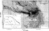 |
Fig. 1 Dust extinction through the Ophiuchus molecular cloud, derived using the
near-infrared extinction mapping technique and 2MASS data (Paper I). The contours are
drawn at |
3. Results
In this section, we use the column density data introduced in Sect. 2 to examine the nature of the diffuse and dense components. We first examine the physical characteristics of the components, namely the masses and sizes, densities, and velocity structure. Then, we consider the observed characteristics from the point of view of pressure balance in molecular clouds.
3.1. Characteristics of the diffuse and dense components
3.1.1. Total mass
The gas column densities in the clouds can be inferred from the extinction maps using
the measured extinction-to-gas column ratio. We transformed the visual extinction values
in the maps into hydrogen column densities using the relation (Bohlin et al. 1978)  (1)We then calculated the
total mass of the cloud as a sum of extinction values above
AV = 1 mag
(1)We then calculated the
total mass of the cloud as a sum of extinction values above
AV = 1 mag 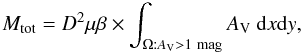 (2)where
D is the distance to the cloud, μ = 1.37 is the mean
molecular weight (adopting the same values as Lombardi
et al. 2008b, i.e., 63% hydrogen, 36% helium, and 1% dust), and
x and y refer to the map pixels. We adopt the same
distances for clouds as listed in Paper I. We note that the chosen lower limit of
AV = 1 mag is arbitrary, and the total mass depends on the
selected value (choosing a lower threshold will yield higher masses for all clouds).
However, a fixed value will make the values comparable between the clouds. We also note
that the AV = 1 mag contour is closed in most mapped
regions, which therefore uniformly defines a cloud boundary. Table 1 lists the mean extinctions,
(2)where
D is the distance to the cloud, μ = 1.37 is the mean
molecular weight (adopting the same values as Lombardi
et al. 2008b, i.e., 63% hydrogen, 36% helium, and 1% dust), and
x and y refer to the map pixels. We adopt the same
distances for clouds as listed in Paper I. We note that the chosen lower limit of
AV = 1 mag is arbitrary, and the total mass depends on the
selected value (choosing a lower threshold will yield higher masses for all clouds).
However, a fixed value will make the values comparable between the clouds. We also note
that the AV = 1 mag contour is closed in most mapped
regions, which therefore uniformly defines a cloud boundary. Table 1 lists the mean extinctions,
 , for the clouds
calculated with this definition for a cloud.
, for the clouds
calculated with this definition for a cloud.
The total mass of the dense component was calculated from the extinction in excess to
the
threshold level: ![Mathematical equation: \begin{equation} \label{eq:mass_dense}M_\mathrm{dense} = D^2 \mu \beta \times \left[\int_{\Omega : A_\mathrm{V} > A_\mathrm{V}^\mathrm{tail}}{A_\mathrm{V}\ \mathrm{d}x \mathrm{d}y} - A_\mathrm{V}^\mathrm{tail} \times \int_{\Omega : A_\mathrm{V} > A_\mathrm{V}^\mathrm{tail}}{\mathrm{d}x \mathrm{d}y}\right]. \end{equation}](/articles/aa/full_html/2011/06/aa16383-10/aa16383-10-eq32.png) (3)The mass of the
diffuse component was then defined as
Mdiffuse = Mtot − Mdense.
We list in Table 1 the ratios of the dense
component mass to the total mass of the cloud. Clearly, the mass of the diffuse
component dominates the cloud mass in all clouds. The ratios vary from a few percents
for clouds with low star-forming activity to ~20% for the most active clouds. Note
that the total mass of the cloud was calculated as the mass above
AV > 1 mag. Because the column
density below this level is, of course, not zero, our total masses represent lower
limits. Accordingly, the quoted
Mdense/Mtot
ratios represent upper limits.
(3)The mass of the
diffuse component was then defined as
Mdiffuse = Mtot − Mdense.
We list in Table 1 the ratios of the dense
component mass to the total mass of the cloud. Clearly, the mass of the diffuse
component dominates the cloud mass in all clouds. The ratios vary from a few percents
for clouds with low star-forming activity to ~20% for the most active clouds. Note
that the total mass of the cloud was calculated as the mass above
AV > 1 mag. Because the column
density below this level is, of course, not zero, our total masses represent lower
limits. Accordingly, the quoted
Mdense/Mtot
ratios represent upper limits.
Molecular clouds and the derived properties.
3.1.2. Clumps in the dense component
In the following, we characterize the individual structures, i.e. clumps, in the dense
component. We used a simple thresholding approach for identifying the clumps from the
extinction maps, namely the “clumpfind2d” routine (Williams et al. 1994). All pixels in the map that are connected with each
other and above are
considered as one clump. We emphasize that we made no effort to identify single-peaked
structures nested inside the contour defined by ,
because we particularly aimed to examine the mean physical parameters inside regions
defined by the
threshold. Therefore, there can be numerous distinct column density peaks (of any column
density higher than ) nested
inside the clumps. In terms of the clumpfind2d algorithm, this approach equals using
as a
threshold level for structure detection, but not defining any additional column density
levels that would be used in detecting peaks inside this parental structure.
This exercise identified about 10 clumps from each cloud complex that show wide ranges
of sizes and masses. The effective radii of the clumps, defined as
 where A is the area, varies between ~0.1−3 pc. Figure 2 shows the size distribution of all clumps in all
clouds, showing that smaller regions are always more numerous than larger ones down to
the resolution limit of our data (R ≈ 0.1 pc). The size distribution
has a power-law-like shape with the approximate slope of −0.9 ± 0.2.
Figure 2 also shows the mass distribution of the
clumps, calculated by integrating Eq. (3)
over the clump. The mass distribution covers roughly four orders of magnitudes between
10-1−103 M⊙, with a shape
resembling a power-law distribution that has a slope of −0.4 ± 0.2. This slope
is flatter than typically observed for the mass distributions of cores in the clouds
(~−1.3, e.g. Motte et al. 1998; Alves et al. 2007; André et al. 2010), and is closer to the slopes derived for molecular clouds
or CO clumps within individual clouds (~−0.6, e.g. Williams et al. 1995; Kramer et al.
1998; Blitz et al. 2007). It is possible,
however, that the derived slope is affected by the blending of clumps with each other.
This blending can make the detection efficiency of clumps a function of the clump mass,
and thereby affect the slope of the observed mass function (e.g., Kainulainen et al. 2009a; Pineda
et al. 2009). The mass-to-size relation for the clumps, also shown in
Fig. 2, roughly follows the relation
M ∝ R2.7 ± 0.2, which is again
close to what has been derived for CO clumps within clouds (e.g., Carr 1987). The relation also agrees with what is expected for
constant mean volume density spheres and it is steeper than predicted by Larson’s
relations (M ∝ R2). But Larson’s
mean-density size relationship, ρ ∝ R-1 has
been questioned by Ballesteros-Paredes & Mac Low
(2002), who suggested that it is an observational artifact owing to the limited
dynamical range in column density. Our mass-radius relation,
M ∝ R2.7 ± 0.2, can also be seen as an
indicator of the fractal dimension of the cloud, D ≈ 2.7 ± 0.2. This
range is consistent with the highest values in the range,
D = 2.3−2.7, which was previously found by Elmegreen & Falgarone (1996), indicating fairly space-filling
column density structures (Sánchez et al. 2005;
Federrath et al. 2009).
where A is the area, varies between ~0.1−3 pc. Figure 2 shows the size distribution of all clumps in all
clouds, showing that smaller regions are always more numerous than larger ones down to
the resolution limit of our data (R ≈ 0.1 pc). The size distribution
has a power-law-like shape with the approximate slope of −0.9 ± 0.2.
Figure 2 also shows the mass distribution of the
clumps, calculated by integrating Eq. (3)
over the clump. The mass distribution covers roughly four orders of magnitudes between
10-1−103 M⊙, with a shape
resembling a power-law distribution that has a slope of −0.4 ± 0.2. This slope
is flatter than typically observed for the mass distributions of cores in the clouds
(~−1.3, e.g. Motte et al. 1998; Alves et al. 2007; André et al. 2010), and is closer to the slopes derived for molecular clouds
or CO clumps within individual clouds (~−0.6, e.g. Williams et al. 1995; Kramer et al.
1998; Blitz et al. 2007). It is possible,
however, that the derived slope is affected by the blending of clumps with each other.
This blending can make the detection efficiency of clumps a function of the clump mass,
and thereby affect the slope of the observed mass function (e.g., Kainulainen et al. 2009a; Pineda
et al. 2009). The mass-to-size relation for the clumps, also shown in
Fig. 2, roughly follows the relation
M ∝ R2.7 ± 0.2, which is again
close to what has been derived for CO clumps within clouds (e.g., Carr 1987). The relation also agrees with what is expected for
constant mean volume density spheres and it is steeper than predicted by Larson’s
relations (M ∝ R2). But Larson’s
mean-density size relationship, ρ ∝ R-1 has
been questioned by Ballesteros-Paredes & Mac Low
(2002), who suggested that it is an observational artifact owing to the limited
dynamical range in column density. Our mass-radius relation,
M ∝ R2.7 ± 0.2, can also be seen as an
indicator of the fractal dimension of the cloud, D ≈ 2.7 ± 0.2. This
range is consistent with the highest values in the range,
D = 2.3−2.7, which was previously found by Elmegreen & Falgarone (1996), indicating fairly space-filling
column density structures (Sánchez et al. 2005;
Federrath et al. 2009).
The mean volume densities in the clumps, defined as
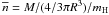 , is on the order of
103 cm-3. The mean volume densities of all clumps in all clouds
have a distribution that peaks strongly at
, is on the order of
103 cm-3. The mean volume densities of all clumps in all clouds
have a distribution that peaks strongly at  cm-3
(shown in Fig. 2). The peak of the distribution is
also relatively narrow, with the mean density being between
cm-3
(shown in Fig. 2). The peak of the distribution is
also relatively narrow, with the mean density being between
 cm-3 for
90% of the clumps. We also calculated the mean density of the diffuse component in the
clouds. This is straightforwardly defined for each cloud without the clumpfinding
process, because the diffuse component is always a uniform structure. Similarly with the
clumps, the volumes of the clouds were calculated using the effective radii
.
The resulting mean densities, listed in Table 1
as well, are
cm-3 for
90% of the clumps. We also calculated the mean density of the diffuse component in the
clouds. This is straightforwardly defined for each cloud without the clumpfinding
process, because the diffuse component is always a uniform structure. Similarly with the
clumps, the volumes of the clouds were calculated using the effective radii
.
The resulting mean densities, listed in Table 1
as well, are  cm-3,
i.e. 5−10 times lower than the mean densities of the clumps identified from the dense
component.
cm-3,
i.e. 5−10 times lower than the mean densities of the clumps identified from the dense
component.
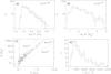 |
Fig. 2 Characteristics of the structures (clumps) defined by a thresholding at
|

3.1.3. Correlation with CO and linewidth
In Fig. 3 we demonstrate how the spatial extent of
the dense component compares to the common molecular line tracer observations. We use as
an example the Ophiuchus and Perseus clouds for which large-scale 12CO and
13CO data are publicly available through the COMPLETE survey (Ridge et al. 2006a). Figure 3 shows the 12CO total antenna temperature map of the
Ophiuchus cloud with a contour of  mag
overplotted. In Ophiuchus, thresholding at
separates two larger clumps: the main cluster region, and the streamers leading east
from the cluster (there are additional clumps identified outside the coverage of the CO
emission). In general, the contour
coincides quite well with the extent of the 12CO line emission data
(1-σ rms error of CO data is 0.98 K), while 13CO is
spatially less extended. Figure 3 also shows a
similar comparison on a smaller spatial scale for the B5 globule in the Perseus cloud.
mag
overplotted. In Ophiuchus, thresholding at
separates two larger clumps: the main cluster region, and the streamers leading east
from the cluster (there are additional clumps identified outside the coverage of the CO
emission). In general, the contour
coincides quite well with the extent of the 12CO line emission data
(1-σ rms error of CO data is 0.98 K), while 13CO is
spatially less extended. Figure 3 also shows a
similar comparison on a smaller spatial scale for the B5 globule in the Perseus cloud.
We identified 10 clumps in the Ophiuchus and Perseus clouds that are fully within the
region covered by the COMPLETE survey. We estimated the virial parameters of these
clumps, defined as the ratio of kinetic-to-gravitational energies in the clump (Bertoldi & McKee 1992):  (4)where
G = 1/232
(4)where
G = 1/232  km s
km s is the gravitational constant and σ the velocity dispersion. The
linewidths were estimated from both the 12CO and 13CO data by
calculating the mean spectrum over the clump and fitting a simple Gaussian to its peak.
The mass was calculated from the extinction data following Eq. (3). This calculation yielded virial
parameters α = 3−100 for the clumps. The virial parameters correlate
with the mass of the clumps approximately in a power-law fashion (Fig. 4). A simple linear least-squares fit to the data
points yields the slopes of −0.69 ± 0.12 and −0.64 ± 0.13 for
12CO and 13CO, respectively. This relation is consistent with
the prediction for clumps confined by ambient pressure from their surrounding medium
(Bertoldi & McKee 1992), and this
relation has been previously observed for clumps identified from CO emission data (e.g.,
Bertoldi & McKee 1992; Williams et al. 1995; Lada et al. 2008). Clearly though, the determination of the virial parameters
suffers from likely nongaussian errors, arising most pressingly from the uncertainty in
determining the linewidth that would well trace most of the gaseous material in the
cloud. Therefore, we consider this observed correlation indicative, although clearly not
well constrained. It is, however, evident that having α ≫ 1, these
clumps are not gravitationally bound entities (although they can be significantly
supported by other forces, as will be discussed later). This is unsurprising, because CO
clumps in molecular clouds are generally observed to have high virial parameters (e.g.,
Carr 1987; Bertoldi & McKee 1992; Falgarone
et al. 1992).
is the gravitational constant and σ the velocity dispersion. The
linewidths were estimated from both the 12CO and 13CO data by
calculating the mean spectrum over the clump and fitting a simple Gaussian to its peak.
The mass was calculated from the extinction data following Eq. (3). This calculation yielded virial
parameters α = 3−100 for the clumps. The virial parameters correlate
with the mass of the clumps approximately in a power-law fashion (Fig. 4). A simple linear least-squares fit to the data
points yields the slopes of −0.69 ± 0.12 and −0.64 ± 0.13 for
12CO and 13CO, respectively. This relation is consistent with
the prediction for clumps confined by ambient pressure from their surrounding medium
(Bertoldi & McKee 1992), and this
relation has been previously observed for clumps identified from CO emission data (e.g.,
Bertoldi & McKee 1992; Williams et al. 1995; Lada et al. 2008). Clearly though, the determination of the virial parameters
suffers from likely nongaussian errors, arising most pressingly from the uncertainty in
determining the linewidth that would well trace most of the gaseous material in the
cloud. Therefore, we consider this observed correlation indicative, although clearly not
well constrained. It is, however, evident that having α ≫ 1, these
clumps are not gravitationally bound entities (although they can be significantly
supported by other forces, as will be discussed later). This is unsurprising, because CO
clumps in molecular clouds are generally observed to have high virial parameters (e.g.,
Carr 1987; Bertoldi & McKee 1992; Falgarone
et al. 1992).
Figure 4 also shows the size-linewidth relation for the clumps in Ophiuchus and Perseus. The data are scattered with no clear correlation, although similarly with the virial parameter-mass relation determining the correlation is hampered by the small number of clumps. We note that if the size and linewidth are uncorrelated, the relation between the virial parameter and mass established above (α ∝ M−2/3) implies that M ∝ R3, i.e. the mean volume densities of the clumps are constant (see Eq. (4)). Indeed, this agrees with the characteristics of the clumps derived in Sect. 3.1.2, i.e., that the mass-radius relation approximately follows M ∝ R2.7 ± 0.1, and that the mean volume densities of the clumps strongly peak around a characteristic value of ~103 cm-3.
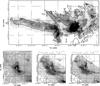 |
Fig. 3 Comparison of the dense component, i.e., structures above
|

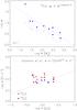 |
Fig. 4 Top: virial parameters derived for clumps identified in the
Ophiuchus and Perseus clouds using thresholding at
|


3.2. Pressure confinement of molecular clumps
As demonstrated in Sect. 3.1.1, the mass in the
clumps above , i.e., in
the dense component, accounts only for the minor fraction of the total gaseous mass of a
cloud. In other words, the clumps are surrounded by a medium whose total mass (and spatial
extent) greatly exceeds that of their own. As an example, the most massive clump in our
cloud sample has about 10% of the mass of the whole cloud (for other clumps, the fraction
is much smaller). Likewise, as shown in Sect. 3.1.2,
the mean density of the clumps is almost an order of magnitude higher than the mean
density of their surrounding medium. Thus, it seems reasonable to consider the external
pressure from the surrounding medium as a force that supports the clumps against
dispersal. Below, we follow the formulation of Bertoldi
& McKee (1992) and examine the scale of external support provided to the
clumps by the diffuse surrounding medium.
The basic condition for the virial balance of a clump is 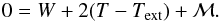 (5)In this equation,
W is the potential energy
(5)In this equation,
W is the potential energy
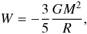 (6)and
T and Text are the kinetic energy of the
clump and its surface term
(6)and
T and Text are the kinetic energy of the
clump and its surface term  ℳ
is the magnetic energy which we neglect for simplicity. The virial balance equation
expressed in terms of pressure is then
ℳ
is the magnetic energy which we neglect for simplicity. The virial balance equation
expressed in terms of pressure is then  (9)In this, the
total kinetic pressure of the clump, Pkin, is the sum of both
thermal and nonthermal components:
(9)In this, the
total kinetic pressure of the clump, Pkin, is the sum of both
thermal and nonthermal components:  (10)and
Pgr is the gravitational pressure of the clump supporting it
against expansion:
(10)and
Pgr is the gravitational pressure of the clump supporting it
against expansion:  (11)Pext
is the external pressure on the clump. Under the assumption that molecular cloud complexes
are close to gravitational virial equipartition (e.g., Larson 1981; Heyer et al. 2001), a
supporting external pressure is directed at a clump. This pressure arises from the
turbulent pressure that balances the cloud against its own gravity. Because the cloud, as
a whole, is close to virial equipartition, the turbulent pressure amounts to the
gravitational pressure of the cloud (analogously to Eq. (11)), but we adopt a slightly modified expression that takes into
account that the cloud is not spherical (Bertoldi &
McKee 1992). With the definition of the mean mass surface density,
(11)Pext
is the external pressure on the clump. Under the assumption that molecular cloud complexes
are close to gravitational virial equipartition (e.g., Larson 1981; Heyer et al. 2001), a
supporting external pressure is directed at a clump. This pressure arises from the
turbulent pressure that balances the cloud against its own gravity. Because the cloud, as
a whole, is close to virial equipartition, the turbulent pressure amounts to the
gravitational pressure of the cloud (analogously to Eq. (11)), but we adopt a slightly modified expression that takes into
account that the cloud is not spherical (Bertoldi &
McKee 1992). With the definition of the mean mass surface density,
 , the external pressure
supporting clumps against dispersal is
, the external pressure
supporting clumps against dispersal is  (12)where
a1 and φG are numerical
constants related to the cloud morphology whose value can be evaluated as prescribed in
Bertoldi & McKee (1992). As an example of
the order-of-magnitude of these pressures, using the typical 13CO linewidth of
σ = 0.75 km s-1 for a R = 1 pc sized clump,
(12)where
a1 and φG are numerical
constants related to the cloud morphology whose value can be evaluated as prescribed in
Bertoldi & McKee (1992). As an example of
the order-of-magnitude of these pressures, using the typical 13CO linewidth of
σ = 0.75 km s-1 for a R = 1 pc sized clump,
 cm-3,
cm-3,
 cm-3, and the mean
mass surface density
cm-3, and the mean
mass surface density  mag
yields the pressure ratios
Pkin ≈ 10 × Pgr ≈ 4 × Pext.
In other words, the pressures supporting the clumps against dispersal amount in total to
about one third of the pressure driving their dispersal.
mag
yields the pressure ratios
Pkin ≈ 10 × Pgr ≈ 4 × Pext.
In other words, the pressures supporting the clumps against dispersal amount in total to
about one third of the pressure driving their dispersal.
Below, we examine these pressures for a population of clumps whose properties equal those
derived for the clumps identified in this paper. In Sect. 3.1.3 we showed that the observed virial parameters of the clumps scale with
their masses (which is predicted for clumps confined by external pressure, Bertoldi & McKee 1992):  (13)where
c1 is a proportionality constant. It directly follows from
this dependence that the internal kinetic pressure of the clumps is only a function of
their density (Eqs. (13) and (11)), and thereby the kinetic pressure is
constant for a population of constant density clumps. The ratio of outward to inward
pressures for a clump is then
(13)where
c1 is a proportionality constant. It directly follows from
this dependence that the internal kinetic pressure of the clumps is only a function of
their density (Eqs. (13) and (11)), and thereby the kinetic pressure is
constant for a population of constant density clumps. The ratio of outward to inward
pressures for a clump is then  (14)Figure 5a illustrates this ratio (Eq. (14)) as a function of the mean mass surface
density
(14)Figure 5a illustrates this ratio (Eq. (14)) as a function of the mean mass surface
density  (in units of
AV) for clumps of different sizes
(R = 0.1−2.1 pc). As the mean density we used the value
(in units of
AV) for clumps of different sizes
(R = 0.1−2.1 pc). As the mean density we used the value
 cm-3 shown above
to be the peak of the mean densities in the clumps (Sect. 3.1.2). Figure 5 shows that the transition
from a regime where structures are unbound to a regime where they are bound occurs around
cm-3 shown above
to be the peak of the mean densities in the clumps (Sect. 3.1.2). Figure 5 shows that the transition
from a regime where structures are unbound to a regime where they are bound occurs around
 mag
(
mag
( M⊙ pc-2)
for clumps over a wide range of sizes (R = 0.1−2.1 pc). This value is
higher than the observed mean mass surface densities by a factor of about ~2 (see
Table 1), and therefore, the external pressure is
lower than the internal kinetic energy of the clump by a factor of ~4.
M⊙ pc-2)
for clumps over a wide range of sizes (R = 0.1−2.1 pc). This value is
higher than the observed mean mass surface densities by a factor of about ~2 (see
Table 1), and therefore, the external pressure is
lower than the internal kinetic energy of the clump by a factor of ~4.
We so far assumed that the kinetic energies of the clumps scale with mass as shown by
Eq. (13). In principle, this scaling is
supported by the linewidth data of clumps, which show fairly constant linewidths
(Fig. 4). This observation is, however, hampered by
the poor statistics we could achieve with the available data. Therefore, we also consider
a case where the kinetic energies of the clumps scale according to a Larson-like
size-linewidth relation (Solomon et al. 1987):
 (15)Again, Fig. 5b shows the ratio of outward to inward pressures for
clumps (Eq. (14)) as a function of mean
mass surface density of the cloud. Using this scaling of kinetic energies, the balance
occurs approximately at the level of the observed mean mass surface density
(
(15)Again, Fig. 5b shows the ratio of outward to inward pressures for
clumps (Eq. (14)) as a function of mean
mass surface density of the cloud. Using this scaling of kinetic energies, the balance
occurs approximately at the level of the observed mean mass surface density
( mag).
While our observations seem to favor kinetic energy scaling with mass (see also discussion
in Sect. 4), this example illustrates the behavior of
the pressure balance in another plausible scaling scheme, suggesting that the external
pressure can indeed be close to the internal kinetic energy of the clumps.
mag).
While our observations seem to favor kinetic energy scaling with mass (see also discussion
in Sect. 4), this example illustrates the behavior of
the pressure balance in another plausible scaling scheme, suggesting that the external
pressure can indeed be close to the internal kinetic energy of the clumps.
Finally, we illustrate the net effect of the pressures on the individual observed clumps
by calculating modified virial parameters for the clumps for which we have CO data. In
this modified virial parameter, we take into account the external pressure on the clumps:
 (16)The modified virial
parameters are shown in Fig. 4 together with the
traditional virial parameters that include only the gravitational and kinetic energies of
the clumps. In agreement with the earlier results, the modified virial parameters are
clearly smaller compared those resulting from Eq. (4), but they are still somewhat larger than unity.
(16)The modified virial
parameters are shown in Fig. 4 together with the
traditional virial parameters that include only the gravitational and kinetic energies of
the clumps. In agreement with the earlier results, the modified virial parameters are
clearly smaller compared those resulting from Eq. (4), but they are still somewhat larger than unity.
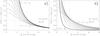 |
Fig. 5 a) Ratio of the pressures supporting a clump against a collapse
(total kinetic pressure) to the pressures promoting it (external and gravitational
pressure) in clumps with |
4. Discussion
4.1. Pressure confinement of the clumps
We described in the previous section a new approach for characterizing structures
observed in molecular clouds. In particular, we used the observed gas column density PDFs
of molecular clouds to define a population of clumpy structures (dense component) embedded
in the extended, interclump medium (diffuse component). The transition between these
components occurs at the extinction threshold mag, or
equivalently, at
Σtail = 40−80 M⊙ pc-2 = 0.008−0.017 g cm-2.
This level is relatively constant and is in the quoted range in every cloud except one
(Serpens, cf. Table 1), for which it could be
reliably determined. The dense component becomes dominant at
AV = 3−8 mag. The mass of the dense component is between
1−20% of the total mass of the cloud, which we defined as the total mass above
AV > 1 mag. The clumps of the dense
component show roughly power-law-like distributions of sizes and masses, covering wide
dynamical ranges (see Fig. 2). However, the
components are characterized by remarkably constant mean volume densities of
cm-3 and
 cm-3 for
the dense and diffuse components, respectively.
cm-3 for
the dense and diffuse components, respectively.
The clumps identified using the column density PDFs of the clouds in this study are very
similar to the gravitationally unbound 13CO clumps identified
in several studies in the past (e.g. Carr 1987;
Bertoldi & McKee 1992; Williams et al. 1995; Lada et al. 2008). In particular, the mean densities and mass-radius and virial
parameter-mass relations derived in Sects. 3.1.2,
3.1.3 agree to what has been derived for such CO
clumps. Similarly, those studies have concluded that the external pressure can be a
significant confining source for these clumps. A simple qualitative comparison between the
clumps defined with the threshold
and 13CO clumps indeed suggests that these approaches may trace quite similar
components in the clouds (see Fig. 3).
It has been suggested previously (Goodman et al.
1998; Caselli et al. 2002) and was more
recently directly observed (Pineda et al. 2010a)
that there appears to be a sharp transition to dynamically coherent objects, or cores, at
the scale where nonthermal motions cascade from the supersonic to the subsonic regime (the
sonic scale, e.g. Vázquez-Semadeni et al. 2003;
Federrath et al. 2010). In particular, Pineda et al. (2010a) detected such a transition in the
B5 globule in the Perseus cloud, at the length scale on the order of
R ≈ 0.1 pc, in agreement with the sonic scale (and Larson’s
size-linewidth relation). The spatial extent of this coherent core is illustrated in
Fig. 3 together with the extent of the clump
defined by . The
transition to coherence clearly occurs in a different column density regime than the break
in the column density PDF defined by .
Importantly, while the structural transition from supersonic- to subsonic velocities in
cloud structure seems to be linked to a particular size-scale, the structural
transition described by the
threshold is not size-dependent. As shown in Fig. 2, structures above cover a
large size- and mass range, with their number decaying in a roughly power-law-like
fashion. Thus, the threshold
appears to be unrelated to the transition to coherent cores in the velocity structure.
Unfortunately, the column density maps used in our work do not provide sufficiently high
spatial resolution to properly sample the PDF at the length scale of the transition to
coherence. Therefore, we were unable to directly look for possible features that the
transition would induce to the PDFs.
We showed in Sect. 3.2 that a significant external
pressure from the surrounding cloud is imposed on the clumps we identified using the
threshold.
This is especially the case if, instead of a constant kinetic pressure, clumps follow a
Larson-like size-linewidth scaling relation. This indicates that the clumps may even be
close to a pressure balance with their surroundings. The CO linewidths and virial
parameters we derived for a small sample of clumps partially support this picture: virial
parameters (as defined by Eq. (4))
correlate with clump masses as predicted for pressure-confined clumps, and the linewidths
show no clear correlation with clump sizes (we observe a nearly constant linewidth for the
clumps). On the other hand, the modified virial parameters that take the external pressure
into account (Fig. 4 and Eq. (16)) were somewhat in excess to unity for
those clumps, implying that they may be over-pressurized and thus either an additional
pressure component may be significantly affecting them, or they may be expanding. This
result is, again, similar to what has been derived for 13CO clumps (e.g., Carr 1987).
The role of the internal gravitational pressure of the clumps is further illustrated in Fig. 6, which shows the mean density for all identified clumps as a function of the clump size (plus signs in the figure). A constant ratio of gravitational-to-external pressures defines a linear relationship in this plot with a slope of −1 (cf. Eqs. (11) and (12)). The relation corresponding to Pgr = Pext is overplotted in Fig. 6. All clumps identified from the dense component have densities lower than this relation, implying that the gravitational energy is indeed low compared to the external pressure. The typical mean density n = 150 cm-3 of the diffuse component is also shown, which obviously is clearly below the mean densities of the clumps.
Despite the limits imposed by the spatial resolution and dynamical range of the
extinction maps, we can still examine the role of gravity in the structures nested inside
the clumps (i.e., in smaller-scale structures inside of what we defined as a clump). We
show in Fig. 6 with red diamonds a population of
structures identified by an experiment in which we defined clumps using a threshold level
 . While
this threshold is typically AV = 6−12 mag, this selection
likely represents a population connected to star-forming regions, or at least, pre-stellar
objects. The structures identified with this experiment are above the
Pgr = Pext line1. This demonstrates how gravitation becomes an
increasingly important confining force for density enhancements nested inside the clumps.
To illustrate one case where gravitation is known to eventually become the dominant force,
we marked in the diagram the star-forming clump B5 in Perseus (see Fig. 3). The clump defined by thresholding at
is marked
with a black filled circle, and the structure identified inside it with the threshold at
. While
this threshold is typically AV = 6−12 mag, this selection
likely represents a population connected to star-forming regions, or at least, pre-stellar
objects. The structures identified with this experiment are above the
Pgr = Pext line1. This demonstrates how gravitation becomes an
increasingly important confining force for density enhancements nested inside the clumps.
To illustrate one case where gravitation is known to eventually become the dominant force,
we marked in the diagram the star-forming clump B5 in Perseus (see Fig. 3). The clump defined by thresholding at
is marked
with a black filled circle, and the structure identified inside it with the threshold at
 is marked
with a red filled circle.
is marked
with a red filled circle.
Given these results, we suggest that the observed organization of structures, identified
with our new approach in using the column density PDF, can be understood as a population
of clumps that are significantly supported by the external pressure. This external
pressure originates from the turbulent pressure outside the clumps, and in this framework,
it is a consequence from the assumption that clouds as a whole are close to virial
equipartition. Then, the break observed in the column density PDFs at
represents
a transition from a diffuse inter-clump medium to clumps significantly supported by
external pressure. This interpretation has some profound implications. Most pressingly, it
implies that the external pressure from the large-scale cloud has an important role in the
formation of molecular cloud structures over wide size and mass scales. This result is
analogous to the recent work of Lada et al. (2008),
who found the external pressure a significant force in confining small-scale cores, or
globules, in the Pipe Nebula. We note that we speculated in Paper I that the transition in
the PDFs could be related to a transition from a regime where gravitation is negligible to
a regime where it is dominant. The results of this paper, however, revise this picture and
more quantitatively connect the break to the pressure conditions of density enhancements
with their surroundings.
We emphasize three main assumptions of this framework. First, we assume that molecular clouds are in virial equilibrium as a whole, in order to relate their gravitational pressure to the turbulent pressure confining the clumps. Although close to being in virial equilibrium, molecular clouds are also embedded in an external medium and may have been formed in large-scale converging flows, which are highly dynamical objects, where surface terms play an important role (see e.g., Ballesteros-Paredes 2006; Banerjee et al. 2009; Schneider et al. 2010). Second, as can be seen from Fig. 5, the external pressure due to the turbulent pressure has a significant role in providing support for the clumps. The confining force exerted to a clump by it, however, depends on the isotropy of the turbulent flow surrounding the clump. Supersonic turbulence is highly anisotropic locally and will lead to transient formation and destruction of filaments and clumps. While estimating the net effect of the turbulent pressure in a more consistent way for each clump would require more detailed velocity information (and modeling of the cloud structure) than are available for this work, we estimated the average level the pressure may have on clumps implicitly in Eq. (12). Third, we neglected the magnetic field stress in our approach. The exact role of the magnetic fields in shaping cloud morphology is still under debate, but generally, it can provide confining pressure perpendicular to the field lines which supports clumps against both collapse and expansion. The magnitude of this support can be estimated roughly with B2/(8π), which generally leads to pressures similar to turbulent ram pressures for the field strengths of B ≈ 15 μG (Crutcher 1999).
Interestingly, Crutcher et al. (2010) recently
found that at densities lower than n ≲ 300 cm-3 the magnetic
field strength do not scale with density, implying that below that density the cloud
material is likely channelled along the field lines. Above this threshold density, the
field strength approximately scales with density as
B ∝ n0.65. In the context of our work, the
threshold density of n ≈ 300 cm-3 is in the regime between the
diffuse component ( cm-3) and the clumps
(
cm-3) and the clumps
( cm-3). This
raises the interesting possibility that the break in the column density PDFs at
would be
related to the change in the role of the magnetic field from dominant at low column
densities to less significant at higher column densities. While Crutcher et al. (2010) suggests that this could be the regime where
cloud structures become self-gravitating, our work rather suggests that this change in the
B-n relation could be caused by a transition to
structures that are not self-gravitating but confined because of their approximate
pressure balance with their surroundings.
cm-3). This
raises the interesting possibility that the break in the column density PDFs at
would be
related to the change in the role of the magnetic field from dominant at low column
densities to less significant at higher column densities. While Crutcher et al. (2010) suggests that this could be the regime where
cloud structures become self-gravitating, our work rather suggests that this change in the
B-n relation could be caused by a transition to
structures that are not self-gravitating but confined because of their approximate
pressure balance with their surroundings.
4.2. Pressure confinement and star formation
When coupled with the main result of Paper I, i.e., that non-star-forming clouds do not exhibit similarly strong tails (if any) in their PDFs as all star-forming clouds do, the interpretation discussed in this paper leads to a picture in which the formation of pressure-confined clumps occurs in clouds prior to (or at a clearly higher rate than) the formation of gravitationally dominated cores. Indeed, in our sample of molecular clouds, pressure confined clumps are observed in some clouds that do not show active star formation (Musca, Cha III), or even high column density cores (Musca et al., in prep.). This picture is further supported by the recent analysis of the stability of dense cores in the nearby, mostly quiescent Pipe Nebula (Lada et al. 2008). In this cloud, Lada et al. examined a sample of ~150 cores of masses between 0.2−20 M⊙ (R ≈ 0.04−0.2 pc). They concluded the core population in the Pipe to be pressure-confined, gravitationally unbound entities. The cores in the Lada et al. study were defined to be single-peaked (or at most a-few-peaked) entities, and thereby they may well represent the smallest scale of the hierarchy whose largest scale is represented by the structures identified in our study. A similar result highlighting the role of external pressure in a star-forming cloud was recently published by Maruta et al. (2010). They investigated the stability of dense cores in the Ophiuchus cluster, in the regime of R ≲ 0.1, and concluded that the external pressure has a significant role in the dynamics of the cores. These results clearly indicate that the hierarchy of structures nested inside clumps is affected by the external pressure all the way to the regime of dense star-forming cores.
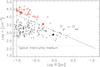 |
Fig. 6 Relation between the mean density and size of the structures (clumps) defined by
thresholding at |
In the interpretation discussed above, the formation of pressure bound clumps can be seen as a prerequisite for the formation of gravitationally bound cores. Given this, there evidently should be a relation between the occurrence of these clumps and star formation, even beyond the general observation that not all quiescent clouds show such clumps, while all star-forming clouds do. Therefore, it is interesting to consider the observed star-forming efficiencies and -rates in the clouds of our sample.
Recently, Heiderman et al. (2010) studied the star-forming activities of nearby molecular clouds as a function of the gas surface density (i.e., the Kennicutt-Schmidt law). In their work, Heiderman et al. used near-infrared extinction maps similar to those employed in this paper to derive gas surface densities. They examined the number of young stellar objects (YSOs) in the clouds identified using the Spitzer satellite data in different column density intervals and constructed the Kennicutt-Schmidt law for their cloud sample. In particular, they observed an abrupt drop in the star-formation rate at Σ ≈ 50−100 M⊙ pc-2 (see Figs. 3 and 8 in Heiderman et al. 2010), which lead them to suggest a threshold for star formation at Σth = 129 ± 14 M⊙ pc-2 (AV = 8.6 mag). A very similar result was recently reached by Lada et al. (2010), who examined the relation between the number of YSOs in nearby clouds and the amount of high column density material in them. They showed that the correlation between the mass of the gas and the number of YSOs identified in the clouds is strongest (i.e., the dispersion in the relation is lowest) at AK ≈ 0.8 mag (AV ≳ 7.3 mag, or Σ ≈ 116 M⊙ pc-1). We note that the dispersion of the SFR-surface density relation derived by Lada et al. (2010) starts to decrease already at surface densities lower than Σ ≈ 116 M⊙ pc-1, reaching its minimum at that point.
The star-formation thresholds derived in the studies above are slightly higher than the
typical values.
However, we defined the value as
the point where the dense component, on average, becomes a significant excess over the
diffuse component. Obviously, at this surface density the largest contribution to the PDF
still comes from the underlying diffuse component, not from the excessive dense component.
Typical surface density values at which the contribution of the tail to the PDF becomes
dominant (>90%) are around
 mag
(listed in Table 1). These values would very well
agree with the threshold values derived by Lada et al.
(2010) and Heiderman et al. (2010),
although very different approaches were used in these papers. Therefore, it seems
plausible to interpret the increase in star-forming activity to be related to the regime
where the column density PDF is becoming completely dominated by the dense component.
mag
(listed in Table 1). These values would very well
agree with the threshold values derived by Lada et al.
(2010) and Heiderman et al. (2010),
although very different approaches were used in these papers. Therefore, it seems
plausible to interpret the increase in star-forming activity to be related to the regime
where the column density PDF is becoming completely dominated by the dense component.
In the context of clumps bound by external pressure, a natural threshold for star
formation is introduced by the surface density at which pressure-bound clumps form, which
is around .
Furthermore, as discussed above, the mass above this threshold is in a direct connection
to the SFR of the cloud, with the SFR increasing in a power-law manner with increasing gas
surface density. This interpretation provides a physically motivated explanation
for the star-formation threshold occurring at relatively low surface densities and links
it to an observed structural feature in the clouds. Thus, we suggest a picture
in which the formation of pressure-bound clumps, and thereby the structural transition at
,
introduces a prerequisite for star formation, with the amount of mass in clouds above that
limit directly proportional to the capability of the cloud to form stars.
5. Conclusions
We presented an analysis of the large-scale, clumpy structures in nearby molecular clouds and of their stability. In particular, we described a new way of identifying the structure in clouds using the observed column density PDFs. With this approach, we identified two distinctive components in them, referred to as the dense and diffuse components, and described their basic physical characteristics. We then examined the stability of the clumps in the dense component, especially by considering the scale of external pressure imposed on them by the surrounding medium. The main conclusions of our work are:
-
1.
The transition between the diffuse and dense components occurs at a narrow range of column densities,
mag, or
Σtail = 40−80 M⊙ pc-2. The
dense component dominates the observed column density PDFs above
AV > 3−8 mag. The total mass
of the dense component is 1−20% of the total mass of the cloud, and thus always
clearly smaller than the mass of the diffuse component. Clumps identified in the dense
component show wide dynamical ranges of sizes (0.1−3 pc) and masses
(10-1−103 M⊙). However, the
mean volume density of the clumps is remarkably constant,
cm-3.
This is ~5−10 times higher than the mean volume density of the diffuse component,
 cm-3.
cm-3.
-
2.
The clumps identified using the column density PDFs are gravitationally unbound and the external pressure, caused by the turbulent pressure from the diffuse, large-scale cloud surrounding them, can provide significant support for them against dispersal. However, examination of the stability of a small subsample of clumps indicates that they may be over-pressurized and either expanding or additionally supported by a component not included in our analysis (e.g. magnetic field support). Then, the physical properties of the clumps resemble those of the clumps often identified from 13CO emission observations as structures of the lowest hierarchical level.
-
3.
In Kainulainen et al. (2009b), we showed that some non-star-forming clouds do not show the PDF break, while some of them show a weak break but no gravitationally dominated dense cores. Coupling those results with the physical characteristics of the clumps derived in this paper suggests a picture in which pressure-confined clumps form prior to, or at higher rate compared to, the formation of gravitationally dominated dense cores in the clouds. This suggests that the formation of pressure-confined clumps is a prerequisite for star formation, and introduces a natural threshold for star formation at
. -
4.
The star-formation rate in the cloud complexes of our sample correlates strongly with the mass in the structures defined by the
threshold,
as pointed out recently by Lada et al. (2010),
and furthermore, drops abruptly below that surface density (Heiderman et al. 2010). This supports the interpretation laid out
in item 3 above. Most importantly, the interpretation then provides a physically
motivated explanation for the relation between star-formation rate and the amount of
dense material in the clouds reported by Heiderman
et al. (2010) and Lada et al. (2010).
Acknowledgments
The authors would like to thank Mordecai-Mark Mac Low, Cornelis Dullemond, and Ralf Klessen for enlightening discussions regarding the topic. We would like to thank the anonymous referee for helping us to significantly improve the manuscript. We would also like to thank Jaime Piñeda for providing electronic material for Fig. 3. C.F. has received funding from the European Research Council under the European Community’s Seventh Framework Programme (FP7/2007-2013 Grant Agreement No. 247060) for the research presented in this work.
References
- Alves, J., Lombardi, M., & Lada, C. J. 2007, A&A, 462, L17 [NASA ADS] [CrossRef] [EDP Sciences] [Google Scholar]
- André, P., Menśhchikov, A., Bontemps, S., et al. 2010, A&A, 518, L102 [NASA ADS] [CrossRef] [EDP Sciences] [Google Scholar]
- Ballesteros-Paredes, J. 2006, MNRAS, 372, 443 [NASA ADS] [CrossRef] [Google Scholar]
- Ballesteros-Paredes, J., & Mac Low, M.-M. 2002, ApJ, 570, 734 [NASA ADS] [CrossRef] [Google Scholar]
- Banerjee, R., Vázquez-Semadeni, E., Hennebelle, P., & Klessen, R. S. 2009, MNRAS, 398, 1082 [NASA ADS] [CrossRef] [Google Scholar]
- Bertoldi, F., & McKee, C. F. 1992, ApJ, 395, 140 [NASA ADS] [CrossRef] [Google Scholar]
- Blitz, L., Fukui, Y., Kawamura, A., et al. 2007, Protostars and Planets V, 81 [Google Scholar]
- Bohlin, R. C., Savage, B. D., & Drake, J. F. 1978, ApJ, 224, 132 [NASA ADS] [CrossRef] [Google Scholar]
- Brunt, C. M. 2010, A&A, 513, A67 [NASA ADS] [CrossRef] [EDP Sciences] [Google Scholar]
- Brunt, C. M., Federrath, C., & Price, D. J. 2010a, MNRAS, 403, 1507 [NASA ADS] [CrossRef] [Google Scholar]
- Brunt, C. M., Federrath, C., & Price, D. J. 2010b, MNRAS, 405, L56 [NASA ADS] [CrossRef] [Google Scholar]
- Burrows, D. N., Singh, K. P., Nousek, J. A., et al. 1993, ApJ, 406, 97 [NASA ADS] [CrossRef] [Google Scholar]
- Butler, M. J., & Tan, J. C. 2009, ApJ, 696, 484 [NASA ADS] [CrossRef] [Google Scholar]
- Cambrésy, L. 1999, A&A, 345, 965 [NASA ADS] [Google Scholar]
- Carr, J. S. 1987, ApJ, 323, 170 [NASA ADS] [CrossRef] [Google Scholar]
- Caselli, P., Benson, P. J., Myers, P. C., & Tafalla, M. 2002, ApJ, 572, 238 [NASA ADS] [CrossRef] [Google Scholar]
- Cho, W., & Kim, J. 2011, MNRAS, 410, L8 [NASA ADS] [Google Scholar]
- Crutcher, R. M. 1999, ApJ, 520, 706 [NASA ADS] [CrossRef] [Google Scholar]
- Crutcher, R. M., Wandelt, B., Heiles, C., et al. 2010, ApJ, 725, 466 [NASA ADS] [CrossRef] [Google Scholar]
- Elmegreen, B. G. 2008, ApJ, 672, 1006 [NASA ADS] [CrossRef] [Google Scholar]
- Elmegreen, B. G., & Falgarone, E. 1996, ApJ, 471, 816 [NASA ADS] [CrossRef] [Google Scholar]
- Falgarone, E., Puget, J.-L., & Perault, M. 1992, A&A, 257, 715 [NASA ADS] [Google Scholar]
- Federrath, C., Glover, S. C. O., Klessen, R. S., & Schmidt, W. 2008a, Phys. Scripta T, 132, 014025 [CrossRef] [Google Scholar]
- Federrath, C., Klessen, R. S., & Schmidt, W. 2008b, ApJ, 688, L79 [NASA ADS] [CrossRef] [Google Scholar]
- Federrath, C., Klessen, R. S., & Schmidt, W. 2009, ApJ, 692, 364 [NASA ADS] [CrossRef] [Google Scholar]
- Federrath, C., Roman-Duval, J., Klessen, R. S., et al. 2010, A&A, 512, A81 [NASA ADS] [CrossRef] [EDP Sciences] [Google Scholar]
- Froebrich, D., & Rowles, J. 2010, MNRAS, 406, 1350 [NASA ADS] [Google Scholar]
- Goodman, A. A., Barranco, J. A., Wilner, D. J., & Heyer, M. H. 1998, ApJ, 504, 223 [NASA ADS] [CrossRef] [Google Scholar]
- Goodman, A. A., Pineda, J. E., & Schnee, S. L. 2009, ApJ, 692, 91 [NASA ADS] [CrossRef] [Google Scholar]
- Heiderman, A., Evans, N. J., II, Allen, L. E., et al. 2010, ApJ, 723, 1019 [NASA ADS] [CrossRef] [Google Scholar]
- Hennebelle, P., & Chabrier, G. 2009, ApJ, 702, 1428 [NASA ADS] [CrossRef] [Google Scholar]
- Heyer, M. H., Carpenter, J. M., & Snell, R. L. 2001, ApJ, 551, 852 [NASA ADS] [CrossRef] [Google Scholar]
- Kainulainen, J., Lehtinen, K., & Harju, J. 2006, A&A, 447, 597 [NASA ADS] [CrossRef] [EDP Sciences] [Google Scholar]
- Kainulainen, J., Lada, C. J., Rathborne, J. M., & Alves, J. F. 2009a, A&A, 497, 399 [NASA ADS] [CrossRef] [EDP Sciences] [Google Scholar]
- Kainulainen, J., Beuther, H., Henning, T., & Plume, R. 2009b, A&A, 508, L35, Paper I [NASA ADS] [CrossRef] [EDP Sciences] [Google Scholar]
- Klessen, R. S. 2000, ApJ, 535, 869 [NASA ADS] [CrossRef] [Google Scholar]
- Kramer, C., Stutzki, J., Rohrig, R., & Corneliussen, U. 1998, A&A, 329, 249 [NASA ADS] [Google Scholar]
- Kritsuk, A. G., Norman, M. L., & Wagner, R. 2011, ApJ, 727, L20 [NASA ADS] [CrossRef] [Google Scholar]
- Krumholz, M. R., & McKee, C. F. 2005, ApJ, 630, 250 [NASA ADS] [CrossRef] [Google Scholar]
- Krumholz, M. R., McKee, C. F., & Tumlinson, J. 2009, ApJ, 699, 850 [NASA ADS] [CrossRef] [Google Scholar]
- Lada, C. J., Muench, A. A., Rathborne, et al. 2008, ApJ, 672, 410 [NASA ADS] [CrossRef] [Google Scholar]
- Lada, C. J., Lombardi, M., & Alves, J. F. 2009, ApJ, 703, 52 [NASA ADS] [CrossRef] [Google Scholar]
- Lada, C. J., Lombardi, M., & Alves, J. F. 2010, ApJ, 724, 687 [NASA ADS] [CrossRef] [Google Scholar]
- Larson, R. B. 1981, MNRAS, 194, 809 [NASA ADS] [CrossRef] [Google Scholar]
- Lombardi, M. 2005, A&A, 438, 169 [NASA ADS] [CrossRef] [EDP Sciences] [Google Scholar]
- Lombardi, M. 2009, A&A, 493, 735 [NASA ADS] [CrossRef] [EDP Sciences] [Google Scholar]
- Lombardi, M., & Alves, J. 2001, A&A, 377, 1023 [NASA ADS] [CrossRef] [EDP Sciences] [Google Scholar]
- Lombardi, M., Alves, J., & Lada, C. J. 2006, A&A, 454, 781 [NASA ADS] [CrossRef] [EDP Sciences] [Google Scholar]
- Lombardi, M., Lada, C. J., & Alves, J. 2008a, A&A, 480, 785 [NASA ADS] [CrossRef] [EDP Sciences] [Google Scholar]
- Lombardi, M., Lada, C. J., & Alves, J. 2008b, A&A, 489, 143 [NASA ADS] [CrossRef] [EDP Sciences] [Google Scholar]
- Lombardi, M., Alves, J., & Lada, C. J. 2010a, A&A, 519, L7 [NASA ADS] [CrossRef] [EDP Sciences] [Google Scholar]
- Lombardi, M., Lada, C. J., & Alves, J. 2010b, A&A, 512, A67 [NASA ADS] [CrossRef] [EDP Sciences] [Google Scholar]
- Mac Low, M.-M., & Klessen, R. S. 2004, Rev. Mod. Phys., 76, 125 [NASA ADS] [CrossRef] [Google Scholar]
- Maruta, H., Nakamura, F., Nishi, R., et al. 2010, ApJ, 714, 680 [NASA ADS] [CrossRef] [Google Scholar]
- McKee, C. F., & Ostriker, E. C. 2007, ARA&A, 45, 565 [NASA ADS] [CrossRef] [Google Scholar]
- Motte, F., Andre, P., & Neri, R. 1998, A&A, 336, 150 [NASA ADS] [Google Scholar]
- Ostriker, E. C., Gammie, C. F., & Stone, J. M. 1999, ApJ, 513, 259 [NASA ADS] [CrossRef] [Google Scholar]
- Ostriker, E. C., Stone, J. M., & Gammie, C. F. 2001, ApJ, 546, 980 [NASA ADS] [CrossRef] [Google Scholar]
- Padoan, P., & Nordlund, Å. 2002, ApJ, 576, 870 [Google Scholar]
- Padoan, P., Nordlund, Å., & Jones, B. J. T. 1997, MNRAS, 288, 145 [NASA ADS] [CrossRef] [Google Scholar]
- Pineda, J. E., Rosolowsky, E. W., & Goodman, A. A. 2009, ApJ, 699, L134 [NASA ADS] [CrossRef] [Google Scholar]
- Pineda, J. E., Goodman, A. A., Arce, H. G., et al. 2010a, ApJ, 712, L116 [NASA ADS] [CrossRef] [Google Scholar]
- Pineda, J. L., Goldsmith, P. F., Chapman, N., et al. 2010b, ApJ, 721, 686 [NASA ADS] [CrossRef] [Google Scholar]
- Ridge, N. A., Di Francesco, J., Kirk, H., et al. 2006a, AJ, 131, 2921 [NASA ADS] [CrossRef] [Google Scholar]
- Ridge, N. A., Schnee, S. L., Goodman, A. A., & Foster, J. B. 2006b, ApJ, 643, 932 [NASA ADS] [CrossRef] [Google Scholar]
- Sánchez, N., Alfaro, E. J., & Pérez, E. 2005, ApJ, 625, 849 [NASA ADS] [CrossRef] [Google Scholar]
- Scalo, J., Vazquez-Semadeni, E., Chappell, D., & Passot, T. 1998, ApJ, 504, 835 [NASA ADS] [CrossRef] [Google Scholar]
- Schneider, N., Csengeri, T., Bontemps, S., et al. 2010, A&A, 520, A49 [NASA ADS] [CrossRef] [EDP Sciences] [Google Scholar]
- Skrutskie, M. F., Cutri, R. M., Stiening, R., et al. 2006, AJ, 131, 1163 [NASA ADS] [CrossRef] [Google Scholar]
- Solomon, P. M., Rivolo, A. R., Barrett, J., & Yahil, A. 1987, ApJ, 319, 730 [NASA ADS] [CrossRef] [Google Scholar]
- Tassis, K., Christie, D. A., Urban, et al. 2010, MNRAS, 408, 1089 [NASA ADS] [CrossRef] [Google Scholar]
- Vázquez-Semadeni, E. 1994, ApJ, 423, 681 [NASA ADS] [CrossRef] [Google Scholar]
- Vázquez-Semadeni, E., & García, N. 2001, ApJ, 557, 727 [NASA ADS] [CrossRef] [Google Scholar]
- Vázquez-Semadeni, E., Ballesteros-Paredes, J., & Klessen, R. S. 2003, ApJ, 585, L131 [NASA ADS] [CrossRef] [Google Scholar]
- Ward-Thompson, D., Kirk, J. M., André, P., et al. 2010, A&A, 518, L92 [NASA ADS] [CrossRef] [EDP Sciences] [Google Scholar]
- Williams, J. P., de Geus, E. J., & Blitz, L. 1994, ApJ, 428, 693 [NASA ADS] [CrossRef] [Google Scholar]
- Williams, J. P., Blitz, L., & Stark, A. A. 1995, ApJ, 451, 252 [NASA ADS] [CrossRef] [Google Scholar]
All Tables
All Figures
|
Fig. 1 Dust extinction through the Ophiuchus molecular cloud, derived using the
near-infrared extinction mapping technique and 2MASS data (Paper I). The contours are
drawn at |
| In the text | |
|
Fig. 2 Characteristics of the structures (clumps) defined by a thresholding at
|
| In the text | |
|
Fig. 3 Comparison of the dense component, i.e., structures above
|
| In the text | |
|
Fig. 4 Top: virial parameters derived for clumps identified in the
Ophiuchus and Perseus clouds using thresholding at
|
| In the text | |
|
Fig. 5 a) Ratio of the pressures supporting a clump against a collapse
(total kinetic pressure) to the pressures promoting it (external and gravitational
pressure) in clumps with |
| In the text | |
|
Fig. 6 Relation between the mean density and size of the structures (clumps) defined by
thresholding at |
| In the text | |
Current usage metrics show cumulative count of Article Views (full-text article views including HTML views, PDF and ePub downloads, according to the available data) and Abstracts Views on Vision4Press platform.
Data correspond to usage on the plateform after 2015. The current usage metrics is available 48-96 hours after online publication and is updated daily on week days.
Initial download of the metrics may take a while.