| Issue |
A&A
Volume 529, May 2011
|
|
|---|---|---|
| Article Number | A17 | |
| Number of page(s) | 15 | |
| Section | Cosmology (including clusters of galaxies) | |
| DOI | https://doi.org/10.1051/0004-6361/201016015 | |
| Published online | 22 March 2011 | |
Massive and refined
II. The statistical properties of turbulent motions in massive galaxy clusters with high spatial resolution
1
Jacobs University Bremen, Campus Ring 1, 28759
Bremen,
Germany
e-mail: f.vazza@jacobs-university.de
2
INAF/Istituto di Radioastronomia, via Gobetti 101, 40129
Bologna,
Italy
3
CINECA, High Performance System Division,
Casalecchio di Reno-Bologna,
Italy
Received:
28
October
2010
Accepted:
10
January
2011
We study the properties of chaotic motions in the intra cluster medium using a set of 20 galaxy clusters simulated with large dynamical range, using the adaptive mesh refinement code ENZO. The adopted setup allows us to study the spectral and spatial properties of turbulent motions in galaxy clusters with unprecedented detail, achieving an maximum available Reynolds number of the order of Re ~ 500−1000 for the largest eddies. We investigated the correlations between the energy of these motions in the intra cluster medium and the dynamical state of the host systems. We find that the statistical properties of turbulent motions and their evolution with time imply that major merger events are responsible for the injection of the bulk of turbulent kinetic energy into the cluster. Turbulence is found to account for ~20−30 per cent of the thermal energy in merging clusters, and ~5 per cent in relaxed clusters. We compare the energies of turbulence and motions in our simulated clusters with upper-limits for real nearby clusters derived from XMM-Newton data. When turbulent motions are compared on the same spatial scales, the data from simulations are well within the range presently allowed by observations. Finally, we comment on the possibility that turbulence may accelerate relativistic particles leading to the formation of giant radio halos in turbulent (merging) clusters. On the basis of our simulations, we confirm the conclusions of previous semi-analytical studies that the fraction of turbulent clusters appears to be consistent with that of clusters hosting radio halos.
Key words: galaxies: clusters: general / large-scale structure of Universe / methods: numerical
© ESO, 2011
1. Introduction
It is generally believed that turbulent motions are generated during the hierarchical assembly of matter in galaxy clusters occurring during mergers and the accretion of satellites.
Mergers between galaxy clusters are very energetic events where a fraction of the kinetic energy of dark matter (DM) halos is transferred into the thermal and kinetic energy. The gas from infalling halos is stripped within cluster cores by the action of ram pressure and several fluid instabilities. This drives turbulent motions, which may eventually transfer energy from large to smaller scales (e.g. Sarazin 2002; Cassano & Brunetti 2005; Subramanian et al. 2006; Brunetti & Lazarian 2007). In addition, the sloshing motions of DM cuspy cores that can occur in the cores of clusters at later stages of merging events can drive turbulent motions (e.g. Markevitch & Vikhlinin 2007; Roediger et al. 2010). Even without considering the process of hierarchical formation, galaxy clusters host several potential sources of turbulent motions in the intra cluster medium (ICM). The activity of AGN detected in the central cluster galaxies may excite turbulence in the cores of the hosting clusters (e.g. Fabian et al. 2003; Rebusco et al. 2005; Scannapieco & Brüggen 2008), as well as in galaxies that cross the cluster atmosphere (e.g. Deiss et al. 1996; Subramanian et al. 2006).
From the theoretical viewpoint, turbulence may have a deep impact on both the physics of the ICM (e.g. Narayan & Medvedev 2001; Shekochihin et al. 2005, 2010; Lazarian 2006; Ruszkowsky & Peng 2010) and the properties of non-thermal components in galaxy clusters (e.g. Subramanian et al. 2006; Brunetti & Lazarian 2007; Brunetti & Lazarian 2011). The presence of turbulent gas motions in the ICM is suggested by measurements of the Faraday rotation of the polarization angle of the synchrotron emission from cluster radio galaxies. These studies show that the magnetic field in the ICM is tangled on a broad range of spatial scales (e.g. Murgia et al. 2004; Vogt & Ensslin 2005; Bonafede et al. 2010; Govoni et al. 2010; Vacca et al. 2010) imply that super-Alfvénic motions are present in the medium. In addition, analyses of X-ray observations for a number of nearby clusters, based on pseudo-pressure maps of cluster cores and the lack of evidence for resonant scattering effects in the X-ray spectra, provided hints of turbulence in the ICM (e.g. Schuecker et al. 2004; Henry et al. 2004; Churazov et al. 2004; Ota et al. 2007). Important constraints on the fraction of the turbulent and thermal energy in the cores of clusters are based on the analysis of the broadening of the lines in the emitted X-ray spectra of cool core clusters (Churazov et al. 2008; Sanders et al. 2010). In several cases, these studies derived interesting upper limits to the ratio of turbulent to thermal energy, on the order of 20 per cent, even if the most stringent limits refer to clusters with very compact cores and are thus sensitive to (the energy of) motions on a scale of a few tens of kpc.
Nowadays, numerical simulations provide a unique way to study the generation and evolution of velocity fields in the ICM on a wide range of scales. Early Eulerian numerical simulations of merging clusters (e.g., Roettiger et al. 1999; Norman & Bryan 1999; Ricker & Sarazin 2001) provided the first reliable representation of the way in which turbulence is injected into the ICM by merger events. More recent works, performing high-resolution Lagrangian (Dolag et al. 2005; Vazza et al. 2006; Valdarnini 2011) and Eulerian re-simulations of galaxy clusters extracted from large cosmological volumes found that a sizable amount of pressure support (i.e. ~10−30 percent of the total pressure inside 0.5 Rvir1) in the ICM can be caused by chaotic motions, provided that the kinematic viscosity in the innermost cluster region is negligible for scales ≥ 10 kpc (Nagai et al. 2007; Iapichino & Niemeyer 2008; Lau et al. 2009; Vazza et al. 2009b; Paul et al. 2011; Burns et al. 2010).
The Adaptive Mesh Refinement technique (AMR) is an optimal approach to study the fluid-dynamics of the evolving ICM with high spatial resolution, and within a fully cosmological framework. This technique represents an efficient way of overcoming the problem of having a too coarse spatial resolution in the central region of collapsed objects, which is typical of fixed mesh Eulerian simulations (e.g. Berger & Colella 1989). The proper triggering of the mesh-refinement criteria in AMR simulations allows us to reach peak resolutions comparable to the Lagrangian (smoothed particles hydrodynamics, SPH) simulations in the innermost cluster regions (e.g., ~ 10−20 kpc), while preserving the shock-capturing nature of the algorithm (e.g. Teyssier 2002).
Studies of cosmological simulations have shown that the use of mesh refinement criteria anchored to the properties of the 3D velocity field in the ICM enhances the numerical description of chaotic motions (e.g. Iapichino & Niemeyer 2008; Vazza et al. 2009b; Vazza et al. 2010b). Furthermore, the adoption of sub-grid modeling to treat the dynamical role played by unresolved gas motions helps us to model the motions more accurately, although their importance in the context of galaxy clusters remains qquite unclear (e.g. Scannapieco & Brüggen 2008; Maier et al. 2009).
In Vazza et al. (2010a, hereafter Paper I), we presented a sample of 20 massive galaxy clusters re-simulated with the code ENZO (Norman et al. 2007) employing an AMR strategy designed to increase the spatial resolution in shocks and turbulent features in the ICM out to distances of ~ 2−3 virial radii from cluster centers2. The general properties of both the thermal gas distribution and shock waves in the sample were discussed in Paper I, in relation to the dynamical history of each cluster object.
In the present paper, we focus on the characterization of the chaotic motions of the ICM in these simulated clusters. Compared to previous works on the same issue, our approach combines a large statistics (which allows us to derive viable correlations between turbulent and dynamical features) with high spatial resolution (which enables to follow the details of the gas dynamics and their spectral properties achieving a good scale separation).
The paper is organized as follows: in Sect. 2, we present the re-simulation technique adopted to produce the sample of clusters, and its general properties. In Sect. 3, we discuss the characterization of turbulent gas motions in the sample, focusing on the radial distribution of turbulent motions within clusters, on the spectral features of the ICM velocity field across the sample, and on the scaling relations found between turbulent energy and the virial parameters of the host clusters. We explore in detail the possible connection between the statistical features of large-scale turbulent motions in our cluster sample and the observed statistics of radio halo emission in Sect. 3.6. We finally summarize our conclusions in Sect. 4.
2. Clusters simulations
Computations presented in this work were performed using the ENZO 1.5 code developed by the Laboratory for Computational Astrophysics at the University of California in San Diego3.
The details for the numerical setup are described in Paper I. In summary, cosmological initial conditions were produced with nested grid/DM particle distributions of increasing mass resolution to achieve a high DM mass resolution (mDM = 6.76 × 10⁸ M⊙) in the region of formation of each cluster, of volume ≈ (5−6 Rvir)3, where Rvir is the final virial radius of each cluster.
The clusters were extracted from several boxes sampling a total cubic cosmic volume of Lbox ≈ 440 Mpc h-1.
We assumed a “concordance” ΛCDM cosmology with Ω0 = 1.0, ΩBM = 0.0441, ΩDM = 0.2139, ΩΛ = 0.742, Hubble parameter h = 0.72, and a normalization of the primordial density power spectrum σ8 = 0.8.
Our runs neglect radiative cooling, star formation, and feedback from AGNs, while re-ionization is treated with a simplified Haardt & Madau (1996) re-ionization model (see Appendix of Paper I for details). The physical modeling of re-ionization in our runs is mainly motivated by the requirement of reproducing realistic shock waves, since re-ionization is expected to play a sizable role in setting the strength of outer accretion shocks (e.g. Vazza et al. 2009a).
The clusters in the sample have total masses higher than 6 × 10¹⁴ M⊙, 12 of them having a total mass above > 1015 M⊙.
Grouping the clusters according to their dynamical state is useful for detecting statistical properties that vary inside the cluster sample. In Paper I, we outlined our procedure to distinguish between “relaxing”, “merging”, and “post merger” systems of our sample, focusing on the total matter accretion history of each halo. According to our definition, this sample contains ten post-merger systems (i.e. clusters with a merger of mass ratio larger than 1/3 for z ≤ 1), six merging clusters at z = 0, and four relaxing clusters (i.e. systems without any evidence of past or ongoing major mergers for z < 1).
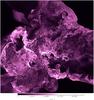 |
Fig. 1 Two dimensional slice showing the gas temperature for the innermost region of galaxy cluster E1, during its main merger event (z = 0.6). The side of the slice is 8.8 Mpc h-1 and the depth along the line of sight is 25 kpc h-1. |
The refinement strategy inside the ≈ (5−6 Rvir)3 volume (hereafter the “AMR region”) was tuned to increase the grid resolution based on the gas/DM over-density, δρgas, DM and/or velocity jumps. In this scheme, a normalized one-dimensional velocity jump across three close cells in the scan direction (at a given refinement level) is computed as δv ≡ |Δv|/|vmin| , where |vmin| is the minimum velocity among the 3 cells and the threshold values used to trigger the mesh refinement were δρgas, DM/ρgas, DM > 3 for gas/DM over-densities and δv > 3 for the 1D velocity jump. For tests about the numerical convergence of this method and a comparison with the more standard refinement based on gas/DM over-density, we address the readers to our previous works (e.g. Vazza et al. 2009b; Vazza 2010b).
The adoption of this refinement criteria was necessary to avoid the spurious suppression of turbulent eddies moving from dense to less dense regions. This is a major drawback of Lagrangian approaches (e.g. SPH, see Dolag et al. 2008, for a review) and of grid methods for which AMR is triggered only by over-density criteria (e.g. Bryan & Norman 1998). In general, the AMR region around each of our clusters at z = 0 is always sampled with at least N ~ 5003 cells at the highest available resolution.
When this extra refinement criterion is adopted, turbulent eddies can evolve with the maximum possible dynamical range, and the decay of turbulence is not artificially damped by numerical under-sampling. A first-order estimate of the Reynolds number available to the largest possible eddies contained within the AMR region yields a value of the order of Re ~ N4/3 ~ 4000 (e.g. Kritsuk et al. 2006). However, based on the velocity power spectra measured for the three-dimensional (3D) velocity field in our clusters (see Sect. 3.3), the maximum Reynolds number achieved in our simulated ICM is the range of Re ~ N4/3 ~ 500−1000. In any case, a rather large hierarchy of chaotic “eddies” of decreasing size can develop within the AMR region and evolve towards the scale of the numerical dissipation, which is a few times the minimum cell size4.
To illustrate the vast amount of spatial details provided by the method employed here, in Fig. 1 we present an example of the pattern of temperature fluctuations in a multiple merger event in one of our forming galaxy clusters (E1), at the time that it assembled the bulk of its total mass (z ~ 0.5−0.6). The side of the slice is ≈ 8.8 Mpc h-1 and the width 25 kpc h-1. The rise of fluid instabilities and vorticity at oblique shocks is evident behind the wake of accretion shocks at the cluster periphery, thanks to the sampling at the peak resolution (25 kpc h-1) even at 4−6 Mpc h-1 from the cluster center. A patchy multi-temperature ICM is observed at this stage of the merger, and a multi-scale distribution of eddies is generated in the core cluster region by the large ~1000−2000 km s-1 relative velocities of the colliding clumps.
The small-scale chaotic components of the ICM flow are highlighted well by detecting the rotational part of the 3D velocity field (e.g. Ryu et al. 2008; Zhu et al. 2010; Paul et al. 2011). Figure 2 shows the map of |∇ × v| for the same region of Fig. 1. We compute the vorticity on the scale of the cells with a simple first-order finite difference method, in which the difference is computed across a baseline scale of lcurl = 50 kpc h-1 in the three directions across each cell. We find that accretion and merger shocks inject a vorticity on the order of ~1000−1500 km s-1 on the scale of lcurl at the location of the outer accretion shocks, while shears along the stripped infalling sub-clumps (e.g. the cold stream of gas entering on the lower right corner in Figs. 1, 2) inject small-scale vorticity at a lower rate, ~300−600 km s-1, but over larger volumes.
3. Results
3.1. The decomposition of “bulk” and “turbulent” motions
To characterize turbulent velocity fields in the complex environment of galaxy clusters, it is necessary to extract the velocity fluctuations from the complex 3D distribution of velocities. This is not a trivial task and a number of different strategies have been adopted to characterize the “bulk” and “turbulent” component of the velocity field. This has been done for instance by taking spherical shell averages (e.g. Bryan & Norman 1999; Iapichino & Niemeyer 2008; Lau et al. 2009; Burns et al. 2010), by mapping in 3D the velocity field on a resolution coarser than the maximum resolution of the simulation (e.g. Dolag et al. 2005; Vazza et al. 2006, 2009b; Valdarnini 2011), or by using sub-grid modeling (e.g. Maier et al. 2009).
In this work, we adopt two different methods to filter the large-scale component of the velocity field of the ICM, and to account for the uncertainty inherent in the particular representation of the turbulent ICM.
In the first method (hereafter the “kMAX” method), we calculate the power spectrum of the 3D velocity field of the ICM and identify the spatial frequency containing most of the kinetic energy in the flow. According to the simplest view of turbulent fluids, this maximum scale kMAX marks the beginning of the energy cascade of turbulent eddies down to the dissipative scale available to the simulation (which is of the order of a few cells at the highest available resolution) and would also represent the scale of the maximum Reynolds number of the flow.
Following Vazza et al. (2009b) and Vazza et al. (2010b), we measured the power spectrum of the velocity field of the simulated ICM, E(k), defined as: 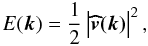 (1)where
  is the Fourier transform of the 3D velocity field (v = [vx,vy,vz]) defined as:
 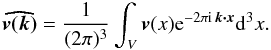 (2)The 3D velocity is measured at the center of (total) mass reference frame, and the power spectrum is calculated by applying a standard FFT algorithm to the data at the highest available resolution, with the addition of a zero-padding technique to deal with the non-periodicity of the considered volume and a Gaussian apodization function to avoid the generation of spurious frequencies at the box edges (see Vazza et al. 2010a; and Valdarnini 2011, for a discussion).
 |
Fig. 3 Maps of the absolute value of the chaotic velocity field for three choices of the coherence scale for Vl (lMAX = 300 kpc, = 600 kpc and = 1200 kpc). The side of the slices is 4 Mpc h-1 and the depth along the line of sight is 25 kpc h-1. |
The power spectrum is measured within a cubic region with side ~4 Rvir centered on each cluster, and the scale kMAX is set to the scale of the maximum value of k·E(k). For every clusters, we filter out the velocity component  with k ≤ kMAX, and consider as “turbulent” only the inverse transform in the real space of the filtered
  . For the clusters of the sample, kMAX is found to correspond to a maximum spatial scale of lMAX ~ 0.75−1.5 Rvir. Since laminar bulk motions of coherence scales smaller than lMAX are not filtered out by this approach, we expect that this method provides an upper limit to the kinetic turbulent energy in the ICM.
In the second method, based on previous works on the same topic (e.g. Dolag et al. 2005; Vazza et al. 2006, 2009b, 2010b), we mapped the 3D velocity field using the fixed spatial scale of lMAX = 300 kpc as a filter to highlight the “turbulent” small-scale features of the ICM. The filtering procedure is applied directly in the real space, by interpolating the original 3D velocity field with a triangular shape cloud kernel (e.g. Hockney & Eastwood 1981) of width lMAX = 300 kpc to map the local mean field, Vl, and to detect turbulent fluctuations on small scales. This is motivated by early studies based on SPH (Dolag et al. 2005), which suggested that the typical size of gas/DM clumps crossing the virial volume of galaxy clusters with M > 1014 M⊙/h at z ~ 0 is <200−300 kpc, and that this filtering scale is therefore suitable to detect velocity fluctuations on scales smaller than the scale of typical laminar infall motion driven by the accreted satellites. However, in the present work we consider larger clusters (by a factor ~10 in total mass and by a factor ~ 3 in Rvir) than previous works. Therefore, a larger physical scale for the injection of turbulent motions by accretion of sub-clumps may by expected and generally yield a lower limit to the estimate of turbulent energy within our simulated clusters.
As an example of the effects of adopting different scales to estimate the turbulent energy budget, in Fig. 3 we show the progressive change introduced by the filtering length used to compute Vl on a cluster simulation. The change in the chaotic field with filtering length l is more evident in the outermost regions, which are also characterized by bulk motions with coherence scales of the order of ~300−500 kpc (see the evolution of the clumps located at the right of the cluster center in Fig. 3). The pattern of motions in the central cluster regions are found to be tangled on scales much smaller than a Mpc, therefore adopting 300 kpc as a filtering length (or more) does not produce significant differences in the reconstructed turbulent velocity field.
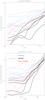 |
Fig. 4 Profiles of the turbulent to total energy ratio for lMAX = 300 kpc (top panel) and for lMAX = 2π/kMAX (lower panel), at z = 0. The different colors refer to clusters with a different dynamical state, as explained in Sect. 2. |
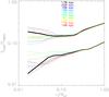 |
Fig. 5 Average profiles of the cumulative turbulent to total energy ratio at z = 0, for nine random displacements from the putative center of mass of the cluster (solid black profiles). The top curves are for a post-merger cluster, the bottom curves for a relaxed cluster. The different colors refer to different displacements from the center (the corresponding absolute values being reported in the panel). |
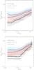 |
Fig. 6 Average profiles of the turbulent to total energy ratio at z = 0, for the 3 dynamical classes of clusters adopting lMAX = 300 kpc for the filtering of the local velocity field (top) or lMAX = 2π/kMAX (bottom). |
In the following, we show that the two filtering techniques produce statistically consistent results when applied to the whole cluster sample, hence the statistical features associated with the turbulent ICM are rather independent of the particular filtering method adopted here.
3.2. Radial distribution of the turbulent energy in the ICM
The ratio of the turbulent energy of the ICM,  (where vt is the “turbulent” velocity field, vt = v − Vl) to the total thermal energy, Etherm = 3/2kBTρ/(μmp) (where T is the gas temperature, kB is the Boltzmann’s constant, μ is the mean molecular mass, and mp is the proton mass) is a simple and important proxy of the importance played by turbulent motions in clusters dynamics.
Figure 4 shows the behavior of the cumulative ratio Eturb/Etherm inside a given radius for all the clusters in the sample at z = 0; for clarity, we show with different colors the three dynamical classes discussed in Sect. 2, and normalize all radii to the Rvir of each cluster. All systems show a profile that increases with radius, with the smallest values of Eturb/Etherm (in the range <10−20 per cent for most of clusters) inside 0.1 Rvir. This ratio reaches larger values at Rvir of Eturb/Etherm ~ 0.5−0.6. In the case of relaxed systems, the turbulent energy stored inside the core region of the clusters can be as small as ~5 per cent, while in merging or post-merger systems it can be as large as ~20−30 per cent. Inside 0.1 Rvir, two systems have Eturb/Etherm > 0.3 with both methods, while inside 0.5 Rvir four (seven) clusters have Eturb/Etherm > 0.3 if the filtering is done using lMAX = 300 kpc (lMAX = 2π/kMAX).
Some caution should be taken in analyzing the radial distribution of turbulence of Fig. 4 in the innermost cluster regions (r < 0.1 Rvir), since the characterization of the center of mass of some systems may be subject to uncertainties, particularly in the case of major merger events. In these cases, asymmetries in the matter distribution and large (~100 kpc) displacements between the centers of gas matter and DM can cause uncertainties in the characterization of the cluster centers. In this respect, to test the stability of our results, we measure the radial distribution of Eturb/Etherm (lMAX = 300 kpc) assuming nine different random centers extracted inside a sphere of ≈ 250 kpc around the peak of total mass, for a post-merger cluster and for a relaxed one (Fig. 5). In both systems, the differences in the estimated turbulent energy ratio inside r < 0.1 Rvir can be as large as a factor ~2−3; however, even in the case of the perturbed system a good convergence in the estimated Eturb/Etherm is achieved for r ~ 0.1 Rvir, even for extreme values of the assumed displacement from the “real” cluster centers. With this caveat in mind, in what follows we focus mainly on the integrated values of Eturb/Etherm at radii larger than r > 0.1 Rvir, observing that in general the differences between the dynamical classes of clusters are larger than the uncertainty associated with the exact location of the cluster center.
Overall, when compared outside the innermost region, the profiles of turbulent energies in both SPH simulations of galaxy clusters (e.g. Dolag et al. 2005; Valdarnini 2011) and AMR grid simulations as given here (see also Iapichino & Niemeyer 2008; Vazza et al. 2009b) are closely similar. However, small systematic differences are present, because of the different ways in which gas matter from infalling clumps is stripped in the two methods (e.g. Agertz et al. 2007) and the different stratification of gas entropy within the inner cluster atmosphere, which in turn affects the stability to convective motions in the ICM (e.g. Wadsley et al. 2008; Mitchell et al. 2008; Springel 2010; Vazza 2011).
To describe more general features of the three dynamical classes of clusters, we computed the average profiles of all the cluster within each subsample, as shown in Fig. 6. Merging, post-mergers and relaxing systems define a “sequence”, with the latter being less turbulent within the virial volume. The larger values of Eturb/Etherm in merging systems suggest that the generation of turbulence starts before the close encounter of cluster cores. In Fig. 7, we show the evolution of gas temperature and total gas velocity for a slice of depth 25 kpc h-1 through the merging axis of the major merger cluster E26, for the epochs of z = 0.79, 0.59, and 0.28 (the closest core encounters happen at z ~ 0.3). The actual major merger is anticipated by a number of minor mergers of gas/DM matter flowing along the massive big filament that connects the two clusters, triggering shocks and chaotic motions in the cluster outskirts. The virialization of the outer ICM is much less efficient than that at the center, and lowe compared to the innermost ICM, therefore it is easier to drive transonic turbulent motions that eventually sink towards the center of the post-merger clusters.
We analyzed the merger sequence of this system by computing the average values of gas temperature, gas turbulent velocity, and Eturb/Etherm in a cylinder of radius ≈ 300 kpc along the axis of merger (Fig. 8). At the beginning of the merger, even if the turbulent velocity can be fairly small (~50−100 km s-1), the energy ratio reaches large values (Eturb/Etherm ~ 0.4 at z ≈ 0.8) due to cold gas falling from the outskirts of the two clusters. During the later stages of the collision, the heating of merger shock waves increases the temperature of the ICM and decreases the ratio Eturb/Etherm, even if the turbulent velocity field experiences an overall increase (~200 km s-1 for z < 0.3). This behavior highlights that the ratio of turbulent energy to thermal energy does not always mirror a change in the absolute turbulent energy/velocity, especially for those regions (or stages) in which the ICM is in a highly un-virialized state.
A qualitatively similar complex picture of galaxy clusters in a pre-merger phase has also been suggested by a few X-ray/optical observations (e.g. Murgia et al. 2010; Maurogordato et al. 2011).
3.3. Spectral properties of the gas velocity fields
In Sect. 3.1, we introduced the power spectrum of the 3D velocity field, E(k), as a useful tool for describing the spectral energy distribution of the ICM in our simulations.
Figure 9 shows the average 3D power spectra of all clusters in the sample at z = 0, after averaging each of the three dynamical classes. The spatial frequency k for every cluster has been referred to that corresponding to the virial radius, k0 ≈ 2π/Rvir, while E(k) has been normalized to the total thermal energy inside Rvir. The power spectra follows a well-defined power-law energy distribution for nearly two orders of magnitude in spatial scale, with a slope on the order of α ≤ 5/3−2 (where E(k) ~ k − α). The maximum of E(k) is in the range of ~1−2 Rvir and the drop in the power spectra on larger scales is clearly detected in our runs thanks to the large volume considered. This result basically confirms and extends to higher cluster masses the results obtained in Vazza et al. (2009b) and Vazza et al. (2010b), and shows that the average spectral distribution of the 3D velocity field in evolving galaxy clusters is self-similar across a wide range of virial masses. On spatial scales just below the maximum correlation scale, the slope of the power spectra becomes significantly steeper than the standard α = 5/3 slope of Kolmogorov turbulence, and resembles the Kolmogorov behavior on intermediate spatial scales. This may be explained as the effect of large-scale bulk inflows through the cluster virial radius5, whose kinetic energy adds to the kinetic energy carried by large-scale turbulent motions. A qualitatively similar picture was also provided by ENZO-MHD re-simulations of cluster formation (Xu et al. 2009, 2010). It should also be noticed that the spatial scales smaller than ≤ 8Δ (where Δ is the cell size) are increasingly affected by the numerical dissipation of the parabolic piecewise method employed by ENZO (e.g. Porter & Woodward 1994; Kitsionas et al. 2009). However, the flattening of the spectral slope seen for k/k0 > 20 is not dramatic.
The comparison of the three sub-samples shows that on average merging clusters are characterized by significantly larger coherence scales. This follows from our being able, according to our definition (Paper I), to identify merging systems as those in which a close companion is found, in an early infalling phase. The stronger correlation at ~1−2 Rvir scales follows from the presence of an early stage of interaction between the ICM of colliding massive clusters (see also Fig. 7), whose virial volumes have just begun to cross each other at the moment of observation.
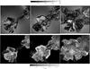 |
Fig. 7 Time evolution for a slice cut through the center of the major merger cluster E26 (from left to right, images are taken at z = 0.79, z = 0.59 and z = 0.28). The bottom panels show the gas temperature, the top ones show the velocity module. The side of each slice is of 8 Mpc h-1. |
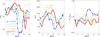 |
Fig. 8 Average gas temperature (left), average turbulent velocity (center), and average energy ratio Eturb/Etherm (right) along the axis of the major merger of cluster E26, for a cylinder of radius ~300 kpc. The different lines and colors correspond to different redshits. |
A complementary tool to measure the spectral features of the turbulent ICM is the structure function of the 3D velocity field. As for the case of the inter stellar medium, the structure functions (of various order) of the velocity field provide a way to compare simulations with the theoretical expectations of the basic theory of turbulent flows (e.g. Kritsuk et al. 2007). In Vazza et al. (2009b), we have also shown that in the case of the simulated ICM the information provided by the transversal and longitudinal structure functions give results that are consistent with the 3D power spectra, showing maximum coherence scales of the ICM flow at ~Rvir, and an overall good consistency with standard expectations from the Kolmogorov scaling S3(l) ~ l (e.g. Kritsuk et al. 2007).
Here we consider the third order structure function of the absolute value of the velocity, | v |  (3)For each cluster, S3 was reconstructed by extracting ~ 106 random pairs of cells within the AMR region and measuring the average (volume-weighted) structure function in every radial bin. Figure 10 shows the average results for the three dynamical classes of clusters. In this case, the distance was rescaled to that of the virial radius of every cluster, while the values of S3 were normalized to
  (where cs is the volume-averaged sound speed inside each cluster virial radius). The maximum of the structure functions is found on the scale of 1−2Rvir, which is consistent with the outer scales provided by the power spectra analysis. A behavior broadly consistent with a linear scaling, S3(l) ~ l0.5−1 is found for all dynamical classes of clusters, within the range of 0.05 ≤ r/Rvir ≤ 1.5.
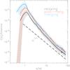 |
Fig. 9 Average power spectra of the 3D velocity field for the different classes of galaxy clusters in our sample, at z = 0. |
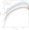 |
Fig. 10 Third order structure functions for |v(r + l) − v(r)| for the dynamical classes of the sample. The spatial scale has been normalized for the virial radius of every cluster, while S3 has been normalized by |
3.4. Scaling laws for the turbulent energy budget in clusters
The injection of chaotic motions by mergers/accretions is a mechanism mainly driven by the gravity of galaxy clusters, and hence overall it should scale with virial cluster parameters. One way to model the turbulence injection in the ICM is to assume that during mergers a fraction of the PdV work done by the sub-clusters infalling onto the main cluster goes into the excitation of turbulent motions (e.g. Cassano & Brunetti 2005). In this case turbulence is injected into the cluster volume swept by the accreted sub-clusters, that is unbound by the effect of the ram pressure stripping. Since the infalling sub-clusters are driven by the gravitational potential, the velocity of the infall should be  times the sound speed of the main cluster. Consequently, the energy density of the turbulence injected during the cluster-crossing should be proportional to the thermal energy density of the main cluster. In addition, the fraction of the volume of the main cluster in which turbulence is injected (the volume swept up by the infalling sub-clusters) depends only on the mass ratio of the two merging clusters, provided that the distribution of the accreted mass-fraction does not strongly depend on the cluster mass (Lacey & Cole 1993). The combination of these points implies that the energy of turbulence should scale with the cluster thermal energy,
 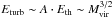 (where A < 1, e.g. Cassano & Brunetti 2005). In agreement with these expectations, Vazza et al. (2006) derived best-fit relations for the scalings between turbulent energy, total virial mass and thermal energy in GADGET2 cosmological simulations, finding
  and Eturb ~ 1/3Eth.
In Fig. 11 we show the scaling between Eturb (measured according to the “kMAX” filtering) and Etherm for three different radii of integration: r < 0.25 Rvir, r < 0.5 Rvir, and r < Rvir. In all cases the scaling closely follows Eturb ∝ Etherm; the scatter however increases when smaller volumes are considered to compute the energies. This supports the idea that the turbulent energy measured in our simulations is a fully gravitationally-driven process, for which the total mass is the driving parameters. However, variations in Eturb/Etherm are found at fixed masses and to depend on the dynamical state of the cluster (see also Sect. 3.5).
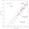 |
Fig. 11 Scaling between the turbulent energy and the thermal energy inside a given radius, for three different radii: < Rvir (squares), < 0.5 Rvir (stars), and < 0.25 Rvir (crosses). The dotted grey line shows the Eturb ∝ Etherm scaling, while the dashed gray line shows the Eturb ~ 0.27Etherm scaling reported in Vazza et al. (2006) for GADGET2 runs. The meaning of colors for the data points is the same as in Fig. 4. |
The turbulent pressure support in the innermost regions of galaxy clusters is important because all estimates of cluster masses derived by X-ray observables are affected by the presence of non-thermal pressure support at some level (Rasia et al. 2004; Lau et al. 2008; Piffaretti & Valdarnini 2008; Burns et al. 2010). Resolved spectra of the chaotic velocity field are beyond the capabilities of existing X-ray facilities, at least for the amount of broadening seen by numerical simulations (e.g. Inogamov & Sunyaev 2003; Dolag et al. 2005; Brüggen et al. 2005; Vazza et al. 2010b). However, a number of upper limits to the amount of turbulent motions in the central region of galaxy clusters (e.g. within the cluster cores) are presently available (e.g. Churazov et al. 2008; Sanders et al. 2010). The comparison between these limits and our simulations provides a sanity check of our results.
Sanders et al. (2011) published upper-limits to the turbulent velocity support available in the central region of 62 nearby galaxy clusters, galaxy groups, and elliptical galaxies. These authors find at least 15 cases where less than ~20 per cent of the thermal energy density is related to turbulence, and weak evidence of turbulent velocities, of the order of ~500 km s-1, in the cool-core cluster RXJ1347.5-1145 that is undergoing a minor merger. We stressed that the results are obtained after modeling and removing the contribution to the broadening of the spatial extent of the objects, which is a difficult task (Sanders et al. 2011, and discussion therein). Nowadays the most “direct” upper limit is likely to be that obtained for A1835, which yields Eturb/Etherm ≤ 0.13 on a scale of ~30 kpc (Sanders et al. 2011).
Although upper limits to turbulence should be treated with caution, in Fig. 12 we plot the upper limits derived from Sanders et al. (2011) for the velocity dispersion versus ICM temperature (as vertical arrows) of the 28 galaxy clusters in their sample, and the results from our simulations (as open squares). The small top squares show the average value of the turbulent velocity field (“kMAX” method), while the connected thick bottom squares show the turbulent energy associated with motion on ≈ 30 kpc scales (which roughly corresponds to the projected volume available to the observations of Sanders et al. 2011). Since the turbulent energy spectrum on the smallest spatial scales in our simulations may be affected by numerical effects in the PPM code on the smallest scales (e.g. Porter & Woodward 1994; and Sect. 3.3), the energy of the turbulent motions on scales ≤ 30 kpc was derived analytically from the measured total power spectrum on larger scales assuming Kolomogorov scaling.
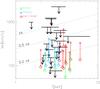 |
Fig. 12 Scaling between the average temperature and the mean velocity dispersion (small squares) for all clusters of the simulated sample (squares in colors) and the cluster observed with XMM-Newton by Sanders et al. (2011). The additional dotted lines show the dependence of the ICM sound speed with the temperature. To compare with the observations, we filtered the velocity for the same spatial coherence scale of l ≈ 30 kpc available to Sanders et al. (2011); the data-point derived in this way are shown as connected thick squares. |
Figure 12 shows that for most of our clusters the measured typical velocity dispersion of motions expected on scales l < 30 kpc is of the order of σv ~ 0.2cs or smaller, well below the upper limits obtained by XMM-Newton. We notice that, even in the case of merging and post-merger systems, where usually very large (l ~ Mpc) chaotic eddies with Eturb/Etherm ~ 0.2−0.3 can develop, the turbulent energy available on the smallest scales is consistent with the upper limits of Sanders et al. (2011). We note however that additional turbulent injection mechanisms connected with AGN outflows are expected to increase the amount of turbulent mixing around cool core clusters (e.g. Brüggen et al. 2005; Heinz et al. 2010; Dubois et al. 2010) and that therefore our estimates here can only be strictly compared with non-cool core clusters. Importantly, as the authors noted, the upper limits reported by Sanders et al. (2011) may be subject to large uncertainties caused by the rather uncertain modeling of the thermal gas distribution around the target sources. Thanks to the high spectral resolution, in a few years Astro-H will likely provide an important tool for improving our understanding of turbulent motions in the ICM (e.g. Takahashi et al. 2010).
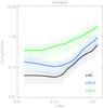 |
Fig. 13 Radial profiles of the Eturb/Etherm ratio for the clusters classified as relaxed at z = 0. |
3.5. Time evolution of turbulence
The evolution of the total mass of each cluster in our sample was presented in Paper I (Fig. 4). These results have shown that the bulk of the total (gas+DM) mass of half of our clusters is built in major merger events at z < 1. This implies that only a few dynamical times have past since the major merger forming our post-merger clusters. Therefore, correlations between turbulent energy and the epoch of the last violent merger should be expected.
To monitor the time-dependent behaviors of turbulence in our cluster sample, we measured the turbulent energy (with the kMAX method) and also the thermal energy for the additional redshifts of z = 0.6 (look-back time of ≈ 5.6 Gyr) and z = 0.3 (≈ 3.3 Gyr). Figure 13 illustrates the evolution of the profile of Eturb/Etherm for the clusters classified as relaxed at z = 0; the averaging procedure is the same as that of Sect. 3.4. These systems have more chaotic motions at all radii with increasing redshift; in particular, at the reference epoch of z = 0.6 their normalized profile is on average rather similar to that of major merger systems at z = 0, suggesting that the ratio Eturb/Etherm depends strictly on the look-back time since the last major merger.
In Fig. 14, we show the values Eturb/Etherm integrated inside spheres of r < 0.25 Rvir and r < Rvir at z = 0.3 and z = 0.6 for all the clusters in our sample (using the “kMAX” method). In addition, in this case the time evolution is rather different when the three dynamical classes are compared. Figure 14 demonstrates the transient feature of turbulence in our simulated clusters: variations in Eturb/Etherm ~ 10 are observed in a few Giga-years in connection with the dynamical status of clusters. Relaxed systems move preferentially “downwards” in the (Etherm,Eturb) plane (i.e. by dissipating their turbulent energy and slightly increasing their thermal energy with time), post-merger systems often have a peak of turbulent injection at intermediate redshifts (due to the merger event they all experience in the 0 ≤ z ≤ 1 range), while merging systems have slightly more irregular paths across the same plane. A very similar behavior is also found by adopting the filter lMAX = 300 kpc (see also Vazza et al. 2006).
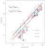 |
Fig. 14 Scaling between the turbulent energy and the thermal energy inside a given radius, as estimated for r < Rvir (top squares) and for r < 0.25 Rvir (lower squares). The dotted gray line shows the Eturb = Etherm scaling, while the long dashed one shows the Eturb = 0.27Etherm best fit relation of Vazza et al. (2006). The meaning of colors is the same as in Fig. 4. |
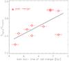 |
Fig. 15 Energy ratio Eturb/Ethermal at z = 0 versus the look-back time of the last merger event for the post-merger systems of the datasample; the horizontal errorbars show the approximate uncertainty in the exact epoch of the central phase of the major merger event for each cluster. |
Figure 15 shows the relation between Eturb/Etherm at z = 0 (inside r < Rvir) and the look-back time of the last major merger, tLM, for the post-merger systems (adopting the “lMAX” method). For these clusters, we can identify the epoch of the last major merger with an uncertainty on the order of a cluster-cluster crossing time (~1−2 Gyr). This figure supports a simple trend between Eturb/Etherm and tLM, of the type Eturb/Etherm ∝ − βtLM, with β ≈ 2/3, and provides additional support to the merger-turbulence connection in our simulated clusters.
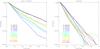 |
Fig. 16 Cumulative volume distribution functions for the ratio of turbulent energy and of thermal energy inside ~1 Mpc3 for two clusters in the sample, by adopting the filtering with lMAX = 300 kpc. |
3.6. On the connection between turbulence and giant radio halos
Radio halos are Mpc synchrotron radio sources detected in the central regions of a fraction of galaxy clusters (Feretti & Giovannini 2000; Kempner & Sarazin 2001; Van Weeren et al. 2009; Ferrari et al. 2008, for a modern review). These emissions are found preferentially in X-ray luminous galaxy clusters (e.g. Giovannini et al. 1999; Venturi et al. 2008; Giovannini et al. 2009) and only in systems with a X-ray perturbed morphology, showing indications of merger activity (Buote 2001). Nowaday’s clear evidence of a statistical connection between cluster mergers and radio halos is provided by present data (Cassano et al. 2010). In principle, several physical mechanisms may contribute to the origin of non-thermal components powering this large-scale radio emission (e.g. Blasi & Colafrancesco 1999; Sarazin 1999; Dolag & Ensslin 2000; Brunetti et al. 2001).
Turbulence in the magnetized ICM may power large-scale radio emission in galaxy clusters, provided that relativistic electrons can couple with the MHD modes excited during merger events (e.g. Brunetti et al. 2008, and references therein). Brunetti & Lazarian (2007, 2011) developed a comprehensive model of the properties of MHD turbulence in the ICM and of the turbulent acceleration of relativistic particles. According to their picture, compressible turbulence provides the most important contribution to the process of particle (turbulent) re-acceleration in the ICM. Under the assumption of a collisional coupling between the turbulent modes and both the thermal and relativistic particles in the ICM, these authors have shown that radio halos can be switched on in massive clusters when compressible turbulence (generated on ~ 300 kpc scales) accounts for ≥ 15−30 per cent of the thermal energy. Although we have shown in Sect. 3.2 that in merging and post-merger clusters, Eturb/Etherm is fairly large, turbulence should also be rather volume filling to produce radio halos of ~ Mpc size.
In Fig. 16, we show the low redshift (z < 0.2) evolution of the cumulative volume distribution of Eturb/Etherm, inside a reference fixed volume of the order of that filled by a typical radio halo (≈ 1 Mpc3) centered on the cluster center of two massive systems of our sample, with nearly identical final mass: a relaxed cluster at z = 0 (right) and a major merger cluster (left). To be conservative in Fig. 16 we used the lMAX = 300 kpc filter, which likely provides a lower limit to the turbulent motions in the ICM.
The fraction of volume where Eturb/Etherm is above a fixed threshold is larger in the post-merger cluster. At z ~ 0, only ~5 per cent of this central volume has Eturb/Etherm > 0.3 in the relaxed cluster, compared to ~30−40 per cent in the post-merger cluster. Although turbulence within the scale length of < 300 kpc does not completely fill the volume even in the post-merger cluster, the whole total “projected” volume within the central 1 Mpc3 of the cluster would be seen as “turbulent” from every line of sight (e.g. Subramanian et al. 2006; Iapichino & Niemeyer 2008). Similar results can be found for all the clusters within the sample, which display a very tight correlation between the volume filling factor of turbulence and the dynamical state of the host galaxy cluster.
Our sample is large enough to allow a first statistical estimate of the frequency of “turbulent” clusters and a first comparison with the observed frequency of radio halos in real galaxy clusters. The cluster-mass distribution of completeness of our sample is consistent with the Press & Schecter mass function for M ≥ 7 × 10¹⁴ M⊙/h; for lower masses, the lack of objects is of the order of ~30 per cent (Fig. 17). This shows that our sample can be safely used for statistical studies provided that our clusters are not biased toward to a particular dynamical state (as in our case, see Paper I).
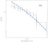 |
Fig. 17 Cumulative mass function for the clusters of our sample (solid line) compared to the theoretical Press-Schecter mass function for the same volume (dashed line). The vertical error bars indicate the Poissonian noise for every mass bin. |
According to calculations of turbulent acceleration in galaxy clusters an energy ratio of  (where TkeV is the cluster temperature measured in keV) may allow the generation of radio halos (Brunetti & Lazarian 2007)6. In Fig. 18 we show the distribution of Eturb/Etherm for the clusters in our sample, evaluated in the typical volume occupied by radio halos. The size of observed radio halos is usually in the range of ~ Mpc, which corresponds to ~ Rvir/3 for most of the clusters in our sample (for completeness, we also report the distribution for r < Rvir/10 and Rvir/2 in the same figure). The cumulative distributions extracted for < Rvir/2 and Rvir/3 are similar for the lMAX = 300 kpc filtering (right panel), while the turbulent energy ratio increases in the lMAX filtering when larger volumes are considered for the integration; this may be due to the large-scale bulk motions present outside the cluster innermost region. Regardless of the filtering technique, about one third of the massive galaxy clusters in the local Universe is found to host turbulent motions of the order of Etherm/4 within Rvir/3. This suggests that the theoretical conditions for the generation of radio halos in our simulated clusters are achieved for ~ 1/3 of our clusters, provided that turbulence drives the formation of diffuse radio emission. Nowadays, extensive radio follow-ups of complete samples of galaxy clusters indicate that a ~ 1/3 of massive LX > 5 × 1044 erg/s (M > 1015 M⊙) objects host Mpc-scale halos (e.g. Venturi et al. 2007, 2008; Cassano et al. 2008) and that all radio halo clusters are merging systems (e.g. Cassano et al. 2010). This is consistent with our previous claim. Semi-analytical calculations based on extended Press-Schechter theory have demonstrated that the theoretical occurrence of Mpc-scale radio halos (assuming that they originate from turbulent acceleration) is consistent with the occurrence of these sources as measured by present surveys (Cassano et al. 2008). This is the first time in which an overall consistency between the fraction of “turbulent” clusters and that of radio-halos clusters in massive objects is underlined by means of numerical cosmological simulations.
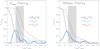 |
Fig. 18 Distribution functions for Eturb/Etherm inside three reference radii (Rvir/2, Rvir/3, and Rvir/10) for the simulated clusters at z = 0. The left panel is for the turbulent ICM velocity field estimated using the lMAX filtering, while the right panel is for the filtering at lMAX = 300 kpc. The solid lines show the differential distributions (for r < Rvir/3 only), while the dashed lines show the cumulative distributions. The vertical gray band shows the approximate regime of turbulence required by calculating the turbulent re-acceleration of relativistic electrons (e.g. Brunetti & Lazarian 2007). |
4. Discussion and conclusions
We have explored the properties of turbulent motions in a statistical sample of massive galaxy clusters simulated at high-resolution with the AMR code ENZO (Norman et al. 2007).
We have focused on a sample of 20 massive galaxy clusters already presented in Paper I and simulated with the tailor-made AMR technique introduced in Vazza et al. (2010b). We have provided a complete view of the onset and the evolution of gravity-driven turbulent motions that are injected into massive galaxy clusters via mergers.
However, the physical modeling adopted in our simulations does not include the effect of AGN activity, cosmic rays and magnetic field. In reality, AGN activity may drive small-scale turbulent motions around the core region of clusters (e.g. Heinz et al. 2006; Scannapieco & Bruggen 2009; Dubois et al. 2010, Morsony et al. 2010; Vazza 2011), while the interplay of a tangled magnetic field and cosmic rays is expected to inject chaotic motions at very small scales, via instabilites in the ICM (Parrish & Stone 2008; Quataert 2008; Ruskowsky & Oh 2010; McCourt et al. 2011; Ruszkowsky et al. 2010).
The magnetic field is also expected to play a role in the cluster evolution (e.g. Dolag 2006; Dubois & Teyssier 2008; Dolag & Stasyszyn 2009; Donnert et al. 2009; Collins et al. 2010), even if without affecting the spectral properties outlined in Sect. 3.3 for a wide range of scales (e.g. Xu et al. 2009, 2010).
The implicit assumption to trust in the development of the turbulent motions derived from our simulations is that kinematic viscosity in the ICM is negligible on all scales larger than the minimum cell size, 25 kpc h-1, which implies that the effective kinematic viscosity, ν, must be smaller than ν ~ 1029 cm2 s-1 7. On smaller scales, there are physical reasons to believe that the turbulence in the ICM is finally dissipated in a collision-less regime, e.g. by accelerating relativistic particles (Brunetti & Lazarian 2007). We have demonstrated that the dynamics of turbulent motions can be accurately modeled on the scales between the numerical resolution of the scheme and the physical scale responsible for dissipation (which is likely ≪ kpc) by means of sub-grid modeling, when assuming some closure relation for the turbulent equations. Valuable attempts have been recently made in the framework of galaxies and galaxy clusters simulations (e.g. Scannapieco & Bruggen 2008; Maier et al. 2009; Iapichino et al. 2010); however, the application of these techniques to astrophysics is still in its infancy.
To summarize our results, the analysis of turbulent motions in this sample of massive galaxy clusters extends the previous results based on the same AMR technique in ENZO and focused on clusters with lower masses (Vazza et al. 2009b, 2010b). Given the fairly large number of objects in this present sample (20), we have been able to study the dependence of the turbulent features on the dynamical state of clusters, following from their matter accretion history across cosmic time. Two methods were presented to detect turbulent motions in the ICM. One is based on a filtering in the Fourier space of the component of velocities associated with wave numbers larger than the wavenumber of the maximum spectral energy, and the other is based on the filtering in the real space of the velocity component with coherence scales smaller than the fixed length of lMAX = 300 kpc. (Sect. 3.1). We have shown that the statistical results obtained in this paper are largely independent of the particular method adopted. Post-merger and merging clusters have large values of turbulent energy compared to the thermal energy of the ICM, with Eturb/Etherm ~ 0.2−0.3 in the innermost cluster regions. On the other hand, relaxed clusters show much lower values of the turbulent ratio, Eturb/Etherm ~ 0.05 (Sect. 3.2) within the same radius. These results are in line with the recent studies of Paul et al. (2011), but extend to clusters with higher masses.
Owing to the very high dynamical range achieved in our simulations (N ~ 550), we have been able to study the spectral features of the ICM velocity field with an unprecedented separation between the forcing and the dissipation scales, achieving a typical Reynolds number of the order of Re ~ 500−1000. The power spectra of the 3D velocity fields extend across nearly two orders of magnitude, with E(k) ~ k−5/3 ÷ −2, and show a typical scale for the peak of the energy spectrum at the scales of 1−2 Rvir (with the tendency of merging clusters to extend across the largest outer correlation scales). Consistent results were also obtained for the measure of the third-order structure function of the velocity field across the cluster sample (Sect. 3.3). As a sanity check, we compared our results with the available limits on turbulent motions in the ICM for X-ray observations (Sanders et al. 2011). We have shown that the available limits on turbulent motions on ~ 10−50 kpc scales obtained in the compact cores of relaxed clusters, Eturb/Etherm < 10 per cent, are consistent with the amount of these motions measured in our simulated clusters (Sect. 3.4). We have derived scaling laws for the integrated turbulent energy in our clusters, and confirm previous results based on GADGET2 runs (Dolag et al. 2005; Vazza et al. 2006), where turbulence is found to scale with the thermal energies (Sect. 3.4). The time evolution of the turbulent energy within clusters was sampled at different epochs (z = 0, z = 0.3, and z = 0.6), and a significant similarity between the turbulence found in the past of relaxed clusters and that found in merging clusters at z = 0 (Sect. 3.5) was identified. We also found an anti-correlation between the look-back time since the last major merger of a cluster and the level of turbulence at z = 0.
Finally we explored the connection between turbulence and radio halos in galaxy clusters. Thanks to the unprecedented large range of statistics for our sample of massive clusters simulated with AMR, we have compared the occurrence of turbulence in our clusters with that of observed giant radio halos in nearby massive clusters. Current calculations of turbulent acceleration for the origin of radio halos suggest that these sources can be generated in the turbulent ICM (e.g. Brunetti & Lazarian 2007). We found that these conditions are reached only in the case of merging systems, where ~1/3 of the cluster volume is in the form of turbulent motions for a few Gyr, while only a few percent of the cluster volume is turbulent in the case of relaxed systems (Sect. 3.6). In particular, we found that ~1/3 of our clusters have Eturb/Etherm > 0.15−0.30 on Mpc-scales and we noted that this fraction is consistent with that of massive clusters hosting giant radio halos. These findings are in line with previous results based on extended Press-Schechter theory, which indicate that the theoretical occurrence of radio halos in the turbulent acceleration model is consistent with present observations.
The generation and evolution of turbulent motions in our simulated ICM is very complex, and follows from the multi-scale energy distribution of the turbulent ICM, as produced by the dynamical evolution of galaxy clusters. It is intriguing that our rather simple physical setup (which does not consider any non-gravitational mechanism) is sufficient to capture some of the most important multi-scale features at work in the turbulent ICM and to produce results in line with existing observations. The adoption of a specially adapted adaptive mesh refinement scheme is mandatory to capture the full range of scales needed to describe the evolution of turbulence in the ICM. However, in the future more sophisticated physical modeling including magnetic fields and cosmic rays would be needed to model the morphological and spectral features of synchrotron radio emission in an accurate and time-dependent way.
In this paper, we adopt the customary definition of the virial radius, Rvir, as the radius enclosing a mean total (gas+DM) overdensity of ≈ 109 times the critical density of the Universe (e.g. Eke et al. 1998).
A public archive of this data-sample is accessible at http://data.cineca.it
For a discussion of the effect of PPM artificial dissipation on the smallest scales in the simulation, see however the discussion in Sect. 3.3.
The motions are likely to be correlated on large scales because of geometrical reasons (see Vazza et al. 2010b).
This can be roughly estimated considering that at the scale of the minimum cell size, Δx = 25 kpc, the typical value of the dispersion in the velocity field is v < 50 km s-1, as shown in Fig. 12, and the Reynolds number is equal to one, and therefore: ν ~ 50 km s-1·25 kpc h-1/Re ~ 1029 cm2 s-1.
Acknowledgments
We acknowledge partial support through grant ASI-INAF I/088/06/0 and PRIN INAF 2007/2008, and the usage of computational resources under the CINECA-INAF 2008-2010 agreement and the 2009 Key Project “Turbulence, shocks and cosmic rays electrons in massive galaxy clusters at high resolution”. F.V. and M.B. acknowledge support from the grant FOR1254 from Deutschen Forschungsgemeinschaft. We thank J. Sanders for kindly making available to us his data points for Fig. 12. We acknowledge very fruitful discussions with S. Ettori, R. Valdarnini, J. Donnert, A. Kritsuk and A. Bonafede. We thank the anonymous referee for his useful comments on this paper. We thank A. J. Brüggen for his late, but fundamental contribution to our work.
References
- Agertz, O., Moore, B., Stadel, J., et al. 2007, MNRAS, 380, 963 [NASA ADS] [CrossRef] [Google Scholar]
- Berger, M. J., & Colella, P. 1989, JCoPh, 82, 64 [Google Scholar]
- Blasi, P., & Colafrancesco, S. 1999, Astrop. Phys., 12, 169 [NASA ADS] [CrossRef] [Google Scholar]
- Bonafede, A., Feretti, L., Murgia, M., et al. 2010, A&A, 513, A30 [NASA ADS] [CrossRef] [EDP Sciences] [Google Scholar]
- Brüggen, M., Hoeft, M., & Ruszkowski, M. 2005, ApJ, 628, 153 [NASA ADS] [CrossRef] [Google Scholar]
- Brunetti, G., & Lazarian, A. 2007, MNRAS, 378, 245 [NASA ADS] [CrossRef] [Google Scholar]
- Brunetti, G., & Lazarian, A. 2011, MNRAS, 412, 817 [NASA ADS] [Google Scholar]
- Brunetti, G., Setti, G., Feretti, L., & Giovannini, G. 2001, MNRAS, 320, 365 [NASA ADS] [CrossRef] [Google Scholar]
- Brunetti, G., Venturi, T., Dallacasa, D., et al. 2007, ApJ, 670, L5 [NASA ADS] [CrossRef] [Google Scholar]
- Brunetti, G., Giacintucci, S., Cassano, R., et al. 2008, Nature, 455, 944 [NASA ADS] [CrossRef] [Google Scholar]
- Bryan, G. L., & Norman, M. L. 1998, ApJ, 495, 80 [NASA ADS] [CrossRef] [Google Scholar]
- Buote, D. A. 2001, ApJ, 553, L15 [NASA ADS] [CrossRef] [Google Scholar]
- Burns, J. O., Skillman, S. W., & O’Shea, B. W. 2010, ApJ, 721, 1105 [Google Scholar]
- Cassano, R., & Brunetti, G. 2005, MNRAS, 357, 1313 [NASA ADS] [CrossRef] [Google Scholar]
- Cassano, R., Brunetti, G., Venturi, T., et al. 2008, A&A, 480, 687 [NASA ADS] [CrossRef] [EDP Sciences] [Google Scholar]
- Cassano, R., Ettori, S., Giacintucci, S., et al. 2010, ApJ, 721, L82 [NASA ADS] [CrossRef] [Google Scholar]
- Churazov, E., Forman, W., Jones, C., Sunyaev, R., & Bohringer, H. 2004, MNRAS, 347, 29 [NASA ADS] [CrossRef] [Google Scholar]
- Churazov, E., Forman, W., Vikhlinin, A., et al. 2008, MNRAS, 388, 1062 [NASA ADS] [CrossRef] [Google Scholar]
- Collins, D. C., Xu, H., Norman, M. L., Li, H., & Li, S. 2010, ApJS, 186, 308 [NASA ADS] [CrossRef] [Google Scholar]
- Deiss, B. M., & Just, A. 1996, A&A, 305, 407 [NASA ADS] [Google Scholar]
- Dolag, K. 2006, Astron. Nachr., 327, 575 [Google Scholar]
- Dolag, K., & Enßlin, T. A. 2000, A&A, 362, 151 [NASA ADS] [Google Scholar]
- Dolag, K., & Stasyszyn, F. 2009, MNRAS, 398, 1678 [NASA ADS] [CrossRef] [Google Scholar]
- Dolag, K., Vazza, F., Brunetti, G., & Tormen, G. 2005, MNRAS, 364, 753 [NASA ADS] [CrossRef] [Google Scholar]
- Dolag, K., Borgani, S., Schindler, S., Diaferio, A., & Bykov, A. M. 2008, SSRv, 134, 229 [NASA ADS] [Google Scholar]
- Donnert, J., Dolag, K., Lesch, H., & Müller, E. 2009, MNRAS, 392, 1008 [NASA ADS] [CrossRef] [Google Scholar]
- Dubois, Y., & Teyssier, R. 2008, A&A, 482, L13 [NASA ADS] [CrossRef] [EDP Sciences] [Google Scholar]
- Dubois, Y., Devriendt, J., Slyz, A., & Teyssier, R. 2010, MNRAS, 409, 985 [NASA ADS] [CrossRef] [Google Scholar]
- Eke, V. R., Cole, S., Frenk, C. S., & Patrick Henry, J. 1998, MNRAS, 298, 1145 [NASA ADS] [CrossRef] [Google Scholar]
- Enßlin, T. A., & Vogt, C. 2006, A&A, 453, 447 [NASA ADS] [CrossRef] [EDP Sciences] [Google Scholar]
- Ferrari, C. 2010 [arXiv:1005.3699] [Google Scholar]
- Giovannini, G., & Feretti, L. 2000, New A, 5, 335 [Google Scholar]
- Giovannini, G., Tordi, M., & Feretti, L. 1999, NewA, 4, 141 [Google Scholar]
- Giovannini, G., Bonafede, A., Feretti, L., et al. 2009, A&A, 507, 1257 [NASA ADS] [CrossRef] [EDP Sciences] [Google Scholar]
- Govoni, F., Dolag, K., Murgia, M., et al. 2010, A&A, 522, A105 [NASA ADS] [CrossRef] [EDP Sciences] [Google Scholar]
- Haardt, F., & Madau, P. 1996, ApJ, 461, 20 [NASA ADS] [CrossRef] [Google Scholar]
- Heinz, S., Brüggen, M., Young, A., & Levesque, E. 2006, MNRAS, 373, L65 [NASA ADS] [CrossRef] [Google Scholar]
- Heinz, S., Brüggen, M., & Morsony, B. 2010, ApJ, 708, 462 [NASA ADS] [CrossRef] [Google Scholar]
- Henry, J. P., Finoguenov, A., & Briel, U. G. 2004, ApJ, 615, 181 [NASA ADS] [CrossRef] [Google Scholar]
- Hockney, R. W., & Eastwood, J. W. 1981, Computer Simulation Using Particles (New York: McGraw-Hill) [Google Scholar]
- Iapichino, L., & Niemeyer, J. C. 2008, MNRAS, 388, 1089 [NASA ADS] [CrossRef] [Google Scholar]
- Iapichino, L., Maier, A., Schmidt, W., & Niemeyer, J. C. 2010, Am. Inst. Phys. Conf. Ser., 1241, 928 [NASA ADS] [Google Scholar]
- Inogamov, N. A., & Sunyaev, R. A. 2003, Astron. Lett., 29, 791 [NASA ADS] [CrossRef] [Google Scholar]
- Kempner, J. C., & Sarazin, C. L. 2001, ApJ, 548, 639 [NASA ADS] [CrossRef] [Google Scholar]
- Kitsionas, S., Federrath, C., Klessen, R. S., et al. 2009, A&A, 508, 541 [NASA ADS] [CrossRef] [EDP Sciences] [Google Scholar]
- Kritsuk, A. G., Norman, M. L., & Padoan, P. 2006, ApJ, 638, L25 [NASA ADS] [CrossRef] [Google Scholar]
- Kritsuk, A. G., Norman, M. L., Padoan, P., & Wagner, R. 2007, ApJ, 665, 416 [NASA ADS] [CrossRef] [Google Scholar]
- Lacey, C., & Cole, S. 1993, MNRAS, 262, 627 [NASA ADS] [CrossRef] [Google Scholar]
- Lau, E. T., Kravtsov, A. V., & Nagai, D. 2009, ApJ, 705, 1129 [NASA ADS] [CrossRef] [Google Scholar]
- Lazarian, A. 2006, ApJ, 645, L25 [NASA ADS] [CrossRef] [Google Scholar]
- Maier, A., Iapichino, L., Schmidt, W., & Niemeyer, J. C. 2009, ApJ, 707, 40 [NASA ADS] [CrossRef] [Google Scholar]
- Markevitch, M., & Vikhlinin, A. 2007, PhR, 443, 1 [Google Scholar]
- Maurogordato, S., Sauvageot, J. L., Bourdin, H., et al. 2011, A&A, 525, A79 [NASA ADS] [CrossRef] [EDP Sciences] [Google Scholar]
- McCourt, M., Parrish, I. J., Sharma, P., & Quataert, E. 2011, MNRAS, accepted [arXiv:1009.2498] [Google Scholar]
- Mitchell, N. L., McCarthy, I. G., Bower, R. G., Theuns, T., & Crain, R. A. 2009, MNRAS, 395, 180 [NASA ADS] [CrossRef] [Google Scholar]
- Morsony, B. J., Heinz, S., Brüggen, M., & Ruszkowski, M. 2010, MNRAS, 407, 1277 [NASA ADS] [CrossRef] [Google Scholar]
- Murgia, M., Govoni, F., Feretti, L., et al. 2004, A&A, 424, 429 [NASA ADS] [CrossRef] [EDP Sciences] [Google Scholar]
- Murgia, M., Govoni, F., Feretti, L., & Giovannini, G. 2010, A&A, 509, A86 [NASA ADS] [CrossRef] [EDP Sciences] [Google Scholar]
- Nagai, D., Kravtsov, A. V., & Vikhlinin, A. 2007, ApJ, 668, 1 [NASA ADS] [CrossRef] [Google Scholar]
- Narayan, R., & Medvedev, M. V. 2001, ApJ, 562, L129 [NASA ADS] [CrossRef] [Google Scholar]
- Norman, M. L., & Bryan, G. L. 1999, The Radio Galaxy Messier, 87, 530, 106 [Google Scholar]
- Norman, M. L., Bryan, G. L., Harkness, R., et al. 2007 [arXiv:0705.1556] [Google Scholar]
- Ota, N., et al. 2007, PASJ, 59, 351 [NASA ADS] [Google Scholar]
- Paul, S., Iapichino, L., Miniati, F., Bagchi, J., & Mannheim, K. 2011, ApJ, 726, 17 [NASA ADS] [CrossRef] [Google Scholar]
- Parrish, I. J., & Quataert, E. 2008, ApJ, 677, L9 [NASA ADS] [CrossRef] [Google Scholar]
- Piffaretti, R., & Valdarnini, R. 2008, A&A, 491, 71 [NASA ADS] [CrossRef] [EDP Sciences] [Google Scholar]
- Porter, D. H., & Woodward, P. R. 1994, ApJS, 93, 309 [NASA ADS] [CrossRef] [Google Scholar]
- Press, W. H., & Schechter, P. 1974, ApJ, 187, 425 [NASA ADS] [CrossRef] [Google Scholar]
- Quataert, E. 2008, ApJ, 673, 758 [NASA ADS] [CrossRef] [Google Scholar]
- Rasia, E., Tormen, G., & Moscardini, L. 2004, MNRAS, 351, 237 [NASA ADS] [CrossRef] [Google Scholar]
- Rebusco, P., Churazov, E., Böhringer, H., & Forman, W. 2005, MNRAS, 359, 1041 [NASA ADS] [CrossRef] [Google Scholar]
- Ricker, P. M., & Sarazin, C. L. 2001, ApJ, 561, 621 [NASA ADS] [CrossRef] [Google Scholar]
- Roediger, E., Brüggen, M., Simionescu, A., et al. 2010 [arXiv:1007.4209] [Google Scholar]
- Roettiger, K., Stone, J. M., & Burns, J. O. 1999, ApJ, 518, 594 [NASA ADS] [CrossRef] [Google Scholar]
- Ruszkowski, M., & Oh, S. P. 2010, ApJ, 713, 1332 [NASA ADS] [CrossRef] [Google Scholar]
- Ruszkowski, M., Lee, D., Bruggen, M., Parrish, I., & Oh, S. P. 2010 [arXiv:1010.2277] [Google Scholar]
- Ryu, D., Kang, H., Cho, J., & Das, S. 2008, Science, 320, 909 [NASA ADS] [CrossRef] [PubMed] [Google Scholar]
- Sanders, J. S., Fabian, A. C., Smith, R. K., & Peterson, J. R. 2010, MNRAS, 402, L11 [Google Scholar]
- Sanders, J. S., Fabian, A. C., & Smith, R. K. 2011, MNRAS, 410, 1797 [NASA ADS] [Google Scholar]
- Sarazin, C. L. 1999, ApJ, 520, 529 [NASA ADS] [CrossRef] [Google Scholar]
- Scannapieco, E., & Brüggen, M. 2008, ApJ, 686, 927 [NASA ADS] [CrossRef] [Google Scholar]
- Schekochihin, A. A., Cowley, S. C., Kulsrud, R. M., Hammett, G. W., & Sharma, P. 2005, ApJ, 629, 139 [NASA ADS] [CrossRef] [Google Scholar]
- Schekochihin, A. A., Cowley, S. C., Rincon, F., & Rosin, M. S. 2010, MNRAS, 405, 291 [NASA ADS] [Google Scholar]
- Schuecker, P., Finoguenov, A., Miniati, F., Böhringer, H., & Briel, U. G. 2004, A&A, 426, 387 [NASA ADS] [CrossRef] [EDP Sciences] [Google Scholar]
- Springel, V. 2005, MNRAS, 364, 1105 [NASA ADS] [CrossRef] [Google Scholar]
- Springel, V. 2010, MNRAS, 401, 791 [NASA ADS] [CrossRef] [Google Scholar]
- Subramanian, K., Shukurov, A., & Haugen, N. E. L. 2006, MNRAS, 366, 1437 [NASA ADS] [CrossRef] [Google Scholar]
- Takahashi, T., et al. 2010, Proc. SPIE, 7732 [Google Scholar]
- Tasker, E. J., Brunino, R., Mitchell, N. L., et al. 2008, MNRAS, 390, 1267 [NASA ADS] [CrossRef] [Google Scholar]
- Teyssier, R. 2002, A&A, 385, 337 [NASA ADS] [CrossRef] [EDP Sciences] [Google Scholar]
- Vacca, V., Murgia, M., Govoni, F., et al. 2010, A&A, 514, A71 [NASA ADS] [CrossRef] [EDP Sciences] [Google Scholar]
- Valdarnini, R. 2011, A&A, 526, A158 [NASA ADS] [CrossRef] [EDP Sciences] [Google Scholar]
- van Weeren, R. J., Röttgering, H. J. A., Brüggen, M., & Cohen, A. 2009, A&A, 508, 75 [NASA ADS] [CrossRef] [EDP Sciences] [Google Scholar]
- Vazza, F. 2011, MNRAS, 410, 461 [NASA ADS] [CrossRef] [Google Scholar]
- Vazza, F., Tormen, G., Cassano, R., Brunetti, G., & Dolag, K. 2006, MNRAS, 369, L14 [NASA ADS] [Google Scholar]
- Vazza, F., Brunetti, G., & Gheller, C. 2009a, MNRAS, 395, 1333 [NASA ADS] [CrossRef] [Google Scholar]
- Vazza, F., Brunetti, G., Kritsuk, A., et al. 2009b, A&A, 504, 33 [NASA ADS] [CrossRef] [EDP Sciences] [Google Scholar]
- Vazza, F., Brunetti, G., Gheller, C., & Brunino, R. 2010a, NewA, 15, 695 [Google Scholar]
- Vazza, F., Gheller, C., & Brunetti, G. 2010b, A&A, 513, A32 [NASA ADS] [CrossRef] [EDP Sciences] [Google Scholar]
- Venturi, T., Giacintucci, S., Brunetti, G., et al. 2007, A&A, 463, 937 [NASA ADS] [CrossRef] [EDP Sciences] [Google Scholar]
- Venturi, T., Giacintucci, S., Dallacasa, D., et al. 2008, A&A, 484, 327 [NASA ADS] [CrossRef] [EDP Sciences] [Google Scholar]
- Vogt, C., & Enßlin, T. A. 2005, A&A, 434, 67 [NASA ADS] [CrossRef] [EDP Sciences] [Google Scholar]
- Zhu, W., Feng, L.-l., & Fang, L.-Z. 2010, ApJ, 712, 1 [NASA ADS] [CrossRef] [Google Scholar]
- Wadsley, J. W., Veeravalli, G., & Couchman, H. M. P. 2008, MNRAS, 387, 427 [NASA ADS] [CrossRef] [Google Scholar]
- Woodward, P., & Colella, P. 1984, JCoPh, 54, 115 [Google Scholar]
- Xu, H., Li, H., Collins, D. C., Li, S., & Norman, M. L. 2009, ApJ, 698, L14 [NASA ADS] [CrossRef] [Google Scholar]
- Xu, H., Li, H., Collins, D. C., Li, S., & Norman, M. L. 2010, ApJ, 725, 2152 [NASA ADS] [CrossRef] [Google Scholar]
All Figures
|
Fig. 1 Two dimensional slice showing the gas temperature for the innermost region of galaxy cluster E1, during its main merger event (z = 0.6). The side of the slice is 8.8 Mpc h-1 and the depth along the line of sight is 25 kpc h-1. |
| In the text | |
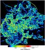 |
Fig. 2 Slice showing the curl of velocity for the same region of Fig. 1. |
| In the text | |
|
Fig. 3 Maps of the absolute value of the chaotic velocity field for three choices of the coherence scale for Vl (lMAX = 300 kpc, = 600 kpc and = 1200 kpc). The side of the slices is 4 Mpc h-1 and the depth along the line of sight is 25 kpc h-1. |
| In the text | |
|
Fig. 4 Profiles of the turbulent to total energy ratio for lMAX = 300 kpc (top panel) and for lMAX = 2π/kMAX (lower panel), at z = 0. The different colors refer to clusters with a different dynamical state, as explained in Sect. 2. |
| In the text | |
|
Fig. 5 Average profiles of the cumulative turbulent to total energy ratio at z = 0, for nine random displacements from the putative center of mass of the cluster (solid black profiles). The top curves are for a post-merger cluster, the bottom curves for a relaxed cluster. The different colors refer to different displacements from the center (the corresponding absolute values being reported in the panel). |
| In the text | |
|
Fig. 6 Average profiles of the turbulent to total energy ratio at z = 0, for the 3 dynamical classes of clusters adopting lMAX = 300 kpc for the filtering of the local velocity field (top) or lMAX = 2π/kMAX (bottom). |
| In the text | |
|
Fig. 7 Time evolution for a slice cut through the center of the major merger cluster E26 (from left to right, images are taken at z = 0.79, z = 0.59 and z = 0.28). The bottom panels show the gas temperature, the top ones show the velocity module. The side of each slice is of 8 Mpc h-1. |
| In the text | |
|
Fig. 8 Average gas temperature (left), average turbulent velocity (center), and average energy ratio Eturb/Etherm (right) along the axis of the major merger of cluster E26, for a cylinder of radius ~300 kpc. The different lines and colors correspond to different redshits. |
| In the text | |
|
Fig. 9 Average power spectra of the 3D velocity field for the different classes of galaxy clusters in our sample, at z = 0. |
| In the text | |
|
Fig. 10 Third order structure functions for |v(r + l) − v(r)| for the dynamical classes of the sample. The spatial scale has been normalized for the virial radius of every cluster, while S3 has been normalized by |
| In the text | |
|
Fig. 11 Scaling between the turbulent energy and the thermal energy inside a given radius, for three different radii: < Rvir (squares), < 0.5 Rvir (stars), and < 0.25 Rvir (crosses). The dotted grey line shows the Eturb ∝ Etherm scaling, while the dashed gray line shows the Eturb ~ 0.27Etherm scaling reported in Vazza et al. (2006) for GADGET2 runs. The meaning of colors for the data points is the same as in Fig. 4. |
| In the text | |
|
Fig. 12 Scaling between the average temperature and the mean velocity dispersion (small squares) for all clusters of the simulated sample (squares in colors) and the cluster observed with XMM-Newton by Sanders et al. (2011). The additional dotted lines show the dependence of the ICM sound speed with the temperature. To compare with the observations, we filtered the velocity for the same spatial coherence scale of l ≈ 30 kpc available to Sanders et al. (2011); the data-point derived in this way are shown as connected thick squares. |
| In the text | |
|
Fig. 13 Radial profiles of the Eturb/Etherm ratio for the clusters classified as relaxed at z = 0. |
| In the text | |
|
Fig. 14 Scaling between the turbulent energy and the thermal energy inside a given radius, as estimated for r < Rvir (top squares) and for r < 0.25 Rvir (lower squares). The dotted gray line shows the Eturb = Etherm scaling, while the long dashed one shows the Eturb = 0.27Etherm best fit relation of Vazza et al. (2006). The meaning of colors is the same as in Fig. 4. |
| In the text | |
|
Fig. 15 Energy ratio Eturb/Ethermal at z = 0 versus the look-back time of the last merger event for the post-merger systems of the datasample; the horizontal errorbars show the approximate uncertainty in the exact epoch of the central phase of the major merger event for each cluster. |
| In the text | |
|
Fig. 16 Cumulative volume distribution functions for the ratio of turbulent energy and of thermal energy inside ~1 Mpc3 for two clusters in the sample, by adopting the filtering with lMAX = 300 kpc. |
| In the text | |
|
Fig. 17 Cumulative mass function for the clusters of our sample (solid line) compared to the theoretical Press-Schecter mass function for the same volume (dashed line). The vertical error bars indicate the Poissonian noise for every mass bin. |
| In the text | |
|
Fig. 18 Distribution functions for Eturb/Etherm inside three reference radii (Rvir/2, Rvir/3, and Rvir/10) for the simulated clusters at z = 0. The left panel is for the turbulent ICM velocity field estimated using the lMAX filtering, while the right panel is for the filtering at lMAX = 300 kpc. The solid lines show the differential distributions (for r < Rvir/3 only), while the dashed lines show the cumulative distributions. The vertical gray band shows the approximate regime of turbulence required by calculating the turbulent re-acceleration of relativistic electrons (e.g. Brunetti & Lazarian 2007). |
| In the text | |
Current usage metrics show cumulative count of Article Views (full-text article views including HTML views, PDF and ePub downloads, according to the available data) and Abstracts Views on Vision4Press platform.
Data correspond to usage on the plateform after 2015. The current usage metrics is available 48-96 hours after online publication and is updated daily on week days.
Initial download of the metrics may take a while.