| Issue |
A&A
Volume 528, April 2011
|
|
|---|---|---|
| Article Number | A45 | |
| Number of page(s) | 5 | |
| Section | Stellar structure and evolution | |
| DOI | https://doi.org/10.1051/0004-6361/201015273 | |
| Published online | 28 February 2011 | |
Bayesian timing analysis of giant flare of SGR 180620 by RXTE PCA
1
Astrophysikalisches Institut und Universitäts-Sternwarte, Universität
Jena,
07745
Jena,
Germany
e-mail: This email address is being protected from spambots. You need JavaScript enabled to view it.
2
Theoretical Astrophysics, Eberhard-Karls-Universität
Tübingen, 72076
Tübingen,
Germany
Received: 24 June 2010
Accepted: 26 December 2010
Abstract
Aims. By detecting high-frequency quasi-periodic oscillations (QPOs) and estimating their frequencies during the decaying tail of giant flares from soft gamma-ray repeaters (SGRs) useful constraints for the equation of state (EoS) of superdense matter may be obtained via comparison with theoretical predictions of eigenfrequencies.
Methods. We used the data collected by the Rossi X-Ray Timing Explorer (RXTE/XTE) Proportional Counter Array (PCA) of a giant flare of SGR 1806−20 on 2004 Dec. 27 and applied an existing Bayesian periodicity detection method to search for oscillations of a transient nature.
Results. In addition to the already detected frequencies, we found a few new frequencies (fQPOs ~ 16.9,21.4,36.4,59.0,116.3 Hz) of predicted oscillations based on the APR14 EoS for SGR 1806−20.
Key words: stars: magnetars / stars: oscillations / X-rays: bursts / methods: data analysis / methods: statistical
© ESO, 2011
1. Introduction
The study of periods of activity of soft gamma-ray repeaters (SGRs, for a recent review see Mereghetti 2008) showing recurrent bursts with subsecond duration and much more extreme events known as giant flares (on rare occasions), may give important input to our understanding of neutron stars (NSs).
In particular, the detection and analysis of quasiperiodic oscillations (QPOs), up to a few kHz, has triggered a number of theoretical studies for prediction and direct comparison with various equations of state (EoS) for superdense matter. These oscillations have been interpreted initially as torsional oscillations of the crust (Samuelsson & Andersson 2007; Sotani et al. 2007), while later the Alfvén oscillations of the fluid core have been taken into account (Levin 2007; Sotani et al. 2008b; Colaiuda et al. 2009; Cerdá-Durán et al. 2009; Hoven & Levin 2011; Gabler et al. 2011; Colaiuda & Kokkotas 2010). These studies suggest how the observations can constrain the mass, the radius, the thickness of the crust, and the strength of magnetic field of NSs. In particular, the timing analysis of the decaying tail of the unprecedent giant flare of SGR 1806−20 on 2004 Dec. 27, allowed detection of QPO frequencies approximately at 18, 26, 30, 92, 150, 625, and 1840 Hz (Israel et al. 2005; Watts & Strohmayer 2006; Strohmayer & Watts 2006; Watts & Strohmayer 2007) in different time intervals, different rotation phases and different amplitudes of oscillations, by means of computation and analysis of the averaged power spectrum.
Here, we present the results of a Bayesian approach to timing analysis of the giant flare data set of SGR 1806−20 registered on 2004 Dec. 27 by RXTE PCA, for detecting a periodic signal of unknown shape and period developed by Gregory & Loredo (1992) (for its sensitivity and advantages see also Gregory & Loredo 1996).
2. Observational data and results of analysis
The giant flare of SGR 1806−20 has been observed by many space-based missions. The data recorded by RXTE PCA instrument consists of five Xenon-filled detectors covering the energy range 2−50 keV and uses the configuration GoodXenon, which records all good events detected in the Xenon chamber with a full timing accuracy of 1 μs. Publicly available data were retrieved by the XTE Data Finder (XDF) user interface (Rots & Hilldrup 1997). Event data files were created and photon arrival times corrected for the solar barycenter using scripts provided in the package XTE ftools. The data set consists of 698 770 registered photons. However, the detectors were saturated during the initial intensive spike phase of the giant flare. For that reason, in our analysis we use the data after ~8.9 s of the flare onset, consisting of ~650 000 photon arrival times, clearly covering 51 rotational cycles of SGR 1806−20 (see Fig. 1).
It is clear that observational detection and parameter estimation of QPO frequencies may play a crucial role for testing any theory predicting eigenfrequencies of the neutron star. In this connection, timing analysis of complex flare data set of SGR 1806−20, with the aim of QPO detection, may be divided into several mutually connected, challenging problems. They include the significance of quasi-periodic signal detection and parameter estimation with high precision. Indeed, the decaying tail of the giant flare of SGR 1806−20 itself has a bumpy structure, very complex light curve shape modulated by rotation of the neutron star (see Fig. 1).
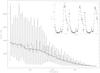 |
Fig. 1 Light curve of the RXTE giant flare of SGR 1806−20 observed on 2004 Dec. 27. The general decay of the giant flare with a bumpy structure on top of it, namely a strongly periodic signal due to rotation (7.56 s). The inset panel shows the rotational modulated light curve (filled circles), together with fitted piecewise constant model (solid line, Hutter 2007), shown here only for 2.5 rotational cycles, with a very complex light curve structure (see text for details). |
The most widely-used procedure for detecting QPOs is an analysis of the power spectrum calculated from the fast Fourier transform (FFT) of uniformly sampled data. Applying the FFT to unevenly spaced, arrival time series data requires binning the data to produce equally spaced samples. Binning is a subjective procedure, because the choice of the bin width and edges can affect the apparent significance of a detection and can limit sensitivity on short time scales. Moreover, the presence of the so-called red-noise (low-frequency signal in the data, i.e. high calculated power can appear at low frequency because of long-timescale features of the data and at high frequencies from higher harmonics of complex shape strong periodic signal) may cause some problems with the interpretation of the results (e.g. Bretthorst 1988). In the previous timing analysis of the giant flare data set of SGR 1806−20 by Israel et al. (2005) and Watts & Strohmayer (2006), an averaged power spectrum was considered. Namely, for each rotational cycle or certain rotational phase interval of SGR 1806−20 an independent classical power spectrum was determined that depends on the phase of rotation and decaying tail of the giant flare, which were subsequently co-added and averaged. This approach divides the data set into small time intervals, which automatically reduces the significance of any periodicity detection of a transient nature and may cause problems related to the windowing of the data sets (van der Klis 1989; Galleani et al. 2001). The complex shape of the light curve (rotational modulation and decaying tail of flare light curves, Fig.1) is properly not taken into account, i.e, by assuming that there are no significant intrinsic variations in the data subsets during small time/phase intervals. Moreover, in some circumstances, FFT may fail to detect the periodic signal (see e.g. Bretthorst 1988; Gregory & Loredo 1996). As explicitly shown by Jaynes (1987) (see also, Bretthorst 1988, 2001; Gregory 2005), the probability for the frequency of a periodic sinusoidal signal is approximately given by ![Mathematical equation: \begin{equation} p(f_n|D,I) \propto \exp\left[\frac{C(f_n)}{\sigma^2}\right], \label{hav} \end{equation}](/articles/aa/full_html/2011/04/aa15273-10/aa15273-10-eq6.png) (1)where C(fn) is the squared magnitude of the FFT, showing that the proper approach toward converting C(fn) into probabilities involves first dividing by the noise variance and then exponentiating, which suppresses spurious ripples in the power spectrum.
(1)where C(fn) is the squared magnitude of the FFT, showing that the proper approach toward converting C(fn) into probabilities involves first dividing by the noise variance and then exponentiating, which suppresses spurious ripples in the power spectrum.
We used a procedure that does not require binning and considers the rotational modulation and decaying tail of the flare (Bretthorst 1988; Gregory & Loredo 1992, 1996; Jaynes & Bretthorst 2003; Vaughan 2010).
For the analysis of the data for the search of QPOs during the giant flare of SGR 1806−20, we applied the Bayesian method developed by Gregory & Loredo (1992) (hereafter referred to as the GL method) to search for pulsed emission from pulsars in X-ray data, consisting of the arrival times of events, when we have no specific prior information about the shape of the signal. The particular case of QPO can be considered a periodic signal with some length of coherence (Q ≡ ν0/2σ, where ν0 is the centroid of the frequency and σ half width at half maximum), i.e. a periodic signal with additional parameters of the oscillation with start and end times1.
The GL method for timing analysis first tests whether a constant, variable, or periodic signal is present in a data set.
In the GL method, periodic models are represented by a signal folded into trial frequency with a light curve shape as a stepwise function with m phase bins per period plus a noise contribution. With such a model we are able to approximate a phase-folded light curve of any shape. Hypotheses for detecting periodic signals represent a class of stepwise, periodic models with the following parameters: trial period, phase, noise parameter, and number of bins (m). The most probable model parameters are then estimated by marginalizing the posterior probability over the prior specified range of each parameter. In Bayesian statistics, posterior probability contains a term that penalizes complex models (unless there is no significant evidence to support that hypothesis), so we calculate the posterior probability by marginalizing over a range of models, corresponding to a prior range of number of phase bins, m, from 2 to 12. Moreover, the GL method is well-suited to variability detection, i.e. to characterize an arbitrary shape light curve with piecewise constant function Z(t) (Rots 2006).
For the search and detection of QPOs, we used a slightly different version of the GL method. First we determined Z(t) – fitting with a piecewise constant model (inset panel of the Fig. 1, Hutter 2007) to characterize the complex light curve shape in the data set, giant flare decaying tail and rotational modulated light curve. Then we subsequently compared competing hypothesis, i.e. whether the data support a purely piecewise constant or piecewise constant+periodic model. If there is an indication of a periodic signal (e.g. odds ratio of competing models exceeding 1, see also Gregory & Loredo (1992, 1996)) we also determined the time intervals where it has its maximum strength (e.g. amplitude or pulsed fraction) via a Markov Chain Monte Carlo (MCMC) approach using QPO start and end times as free parameters.
Finally, in the latter case, we estimate parameters (frequency, phase, amplitude, coherence length of QPO, etc.) of the periodic signal with high precision. For example, in order to estimate the frequency of a periodic signal, the posterior probabilities density function used: 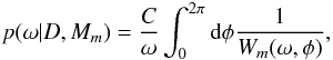 (2)where
 ![Mathematical equation: \hbox{$C=\left[\int_{\omega_{lo}}^{\omega_{hi}}\frac{{\rm d}\omega}{\omega}\int_{0}^{2\pi} {\rm d}\phi \frac{1}{W_m(\omega,\phi)}\right]^{-1}$}](/articles/aa/full_html/2011/04/aa15273-10/aa15273-10-eq14.png) and
and 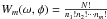 are the normalization constant and number of ways the binned distribution could have arisen “by chance” (nj,j = 1,...,m is the number of events, from the total number of photons–N, falling into the j th of m phase bins given the frequency, ω, and phase, φ, for details, see Gregory & Loredo 1992).
First, we applied the GL method as implemented by Gregory & Loredo (1992) to the 2004 Dec. 27 giant flare whole data set of SGR 1806−20 observed by RXTE PCA and started the timing analysis by performing a blind periodicity search in the range of 12.0–160 Hz. Naturally, we found a very strong coherent signal at ~ 7.56 s, the pulsation period of the NS, followed by higher harmonics up to the 100 Hz (see Fig. 2).
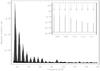 |
Fig. 2 Application of the GL method for a blind periodicity search to the complete data set obtained by RXTE PCA of giant flare of SGR 1806−20 2004 Dec. 27 revealed a strong coherent signal at the frequency of 0.13219244 Hz and higher harmonics up to 100 Hz. Bayesian posterior probability density vs. frequencies in the range of 12.0–160 Hz is shown. The inset panel shows a zoomed part of it around 16.88 Hz. Arrows indicate higher harmonics (from 125 to 132) of the fundamental frequency and the dash-dotted vertical line shows one of the detected QPO frequency in a short time interval (see text, for details). |
Next, we divided the data set into 51 rotational cycles (see Fig. 1). Each of these subsamples were treated as independent data sets. We determined the Bayesian probability densities versus trial frequency. Final probabilities were derived in two ways: first, as the multiplication (the likelihood) of those independent Bayesian posterior probability density functions, and the second one simply summing those independent probabilities2 (see Fig. 3).
This approach also revealed a number of rotational cycles within which the probability of the model of periodic signal is significantly higher than the constant one. Namely, during time intervals of 183.8−191.2, 244.3−251.9 and 259.4−267.1 s, from the flare onset, odd ratios of periodic vs. piece-wise constant models are ~10, ~30, and ~197, correspondingly.
To detect QPO start and end times oscillations, we included also observational data of neighbouring rotational cycles (where an oscillation with that frequency was not detected) and performed the periodicity search for an expanded time interval with additional two free parameters with the MCMC approach with Metropolis-Hastings algorithm. As initial values of these (tQPOstart and tQPOend) parameters served start and end times of an observation, satisfying the condition: tObs.start ≤ tQPOstart < tQPOend ≤ tObs.end. Starting with the abovementioned initial values can be considered as a good strategy, since the detected signal has a higher significance in a subinterval of the considered time interval and the fast convergence of the MCMC procedure already provided. This analysis via MCMC revealed even shorter time intervals within which periodic signal is stronger. The estimates of QPO frequencies and the corresponding 68% interval of the highest probability densities are presented in the Table 1 (see, also Figs. 4, 7).
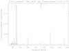 |
Fig. 3 The Bayesian posterior probability density vs. trial frequency of the periodic signal for the giant flare data set of SGR 1806−20. QPO frequencies already detected by averaged power spectrum analysis and also with other mission RHESSI (Israel et al. 2005; Watts & Strohmayer 2006) are marked as small lines at the top axis. Those QPO frequencies are also detected by us. In addition, we have detected several more QPO frequencies (21, 59, and 116 Hz) with the Bayesian method, which were also predicted by Colaiuda et al. (2009). |
Detected QPO frequencies not reported in the literature (Israel et al. 2005; Watts & Strohmayer 2006; Strohmayer & Watts 2006).
As shown by our intensive simulations, this approach readily detects time intervals where the periodic signal has its highest and lowest3 strengths. Nevertheless, we also performed time-frequency analysis (see Figs. 5 and 6, as well as dynamic power spectrum, van der Klis 1989) and candidate QPOs fitted to a Lorentzian function. We estimated frequency centroids and full widths at half maximums. For significant detections they are presented in Table 1. The coherence values Q ≡ ν0/2σ ~ 60–200 indicate the transient nature of almost perfect periodic signals.
For those significant detections, we also fitted folded light curves with a template function, ![Mathematical equation: \hbox{$\psi(t)=\sum_{i=1}^{n} ~A_{i} \sin [i \omega_0(t-\psi_{i})]$}](/articles/aa/full_html/2011/04/aa15273-10/aa15273-10-eq42.png) , truncating the series at the highest harmonic that was statistically significant after performing an F-test (see Dall’Osso et al. 2003, for details). It turned out that oscillations at 16.9 Hz and 36.8 Hz, adding the second harmonic does not improve the fit of the phase-folded light curve (signifcance levels, accordingly are 0.71 and 0.16), while in the case of 21.3 Hz it significantly improves it (significance level of 0.0006. Thus, oscillations at the frequencies of 16.9 Hz and 36.8 Hz can be considered as having sinusoidal shape, and at 21.3 Hz not. We obtained similar results by also analysing power spectra, i.e. fitting spectral profiles of them with sinc function.
, truncating the series at the highest harmonic that was statistically significant after performing an F-test (see Dall’Osso et al. 2003, for details). It turned out that oscillations at 16.9 Hz and 36.8 Hz, adding the second harmonic does not improve the fit of the phase-folded light curve (signifcance levels, accordingly are 0.71 and 0.16), while in the case of 21.3 Hz it significantly improves it (significance level of 0.0006. Thus, oscillations at the frequencies of 16.9 Hz and 36.8 Hz can be considered as having sinusoidal shape, and at 21.3 Hz not. We obtained similar results by also analysing power spectra, i.e. fitting spectral profiles of them with sinc function.
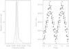 |
Fig. 4 Bayesian posterior probability density vs. frequencies in the time interval of 259–267 s from the giant flare onset. Dashed vertical lines indicate the 68% region of the highest probability density. Odds ratio of periodic vs. constant model is ~200. The right panel depicts the phase-folded light curve with frequency fQPO = 16.88 Hz, with an almost perfect sinusoidal shape (for details, see text). |
3. Discussion
We report the detection of oscillations of transient nature from SGR 1806−20 giant flare decaying tail recorded by the RXTE PCA by applying the GL method for periodicity search. We have confirmed the detections of QPOs at frequencies (in the range of 12−160 Hz) reported by Watts & Strohmayer (2006) and, in addition, found some more QPOs at fQPOs = 16.9,21.4,36.8 Hz with corresponding odds ratios ~197, ~30, and ~10, on shorter time scales, i.e. within individual rotational cycles (see, Fig.7).
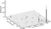 |
Fig. 5 Bayesian posterior probability density vs. frequencies and the time of the giant flare onset. |
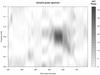 |
Fig. 6 Dynamic power spectrum of giant flare of SGR 1806−20 in the frequency range of 16.5–17.5 Hz and in the time interval of 250–275 s (see, Table 1). |
These odds ratios, describing the significance of a periodic signal, are sensitive to the frequency search range. In contrast, detected frequencies of QPOs, found by locating maximums in the posterior probability density function, are insensitive to the prior search range of frequencies. We computed the uncertainty of fQPOs at 68% confidence level by using this posterior probability density function. In addition to that, we also estimated the significance of our QPO detection by an empirically determined cumulative distribution (see, Fig. 7).
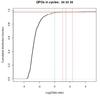 |
Fig. 7 Empirical cumulative distribution function as a function of Odds ratio, i.e. the probability of a periodic model vs. constant one, on the basis of simulations of QPO frequencies with different amplitudes and noise, as much as possible, to the observed values in terms of number of registered photons, spanned times, etc. Detected QPO frequencies are indicated by vertical dashed lines, showing a high significance of detections. |
The broad variety of neutron star oscillation modes (McDermott et al. 1985) is associated with their global structure as well as their internal characteristics. Neutron star seismology has already been proposed as a tool for understanding their internal structure (Kokkotas et al. 2001). The various types of oscillations carry information about the equation of state, the thickness of the crust, the mass, radius, and even the rotation rate (Gaertig & Kokkotas 2010). Still, modelling a truly realistic oscillating neutron star is difficult, although the potential reward is considerable. This has been demonstrated from the recent theoretical results for the QPOs, which have been interpreted as magneto-elastic oscillations. These calculations have shown how the observations constrain the mass, the radius, the thickness of the crust, and the strength of magnetic field of these stars (Sotani et al. 2007; Samuelsson & Andersson 2007; Colaiuda et al. 2009; Cerdá-Durán et al. 2009), while one could even set severe constrains in the geometry of the interior magnetic field (see Sotani et al. 2008a).
In particular, by studying Alfvén oscillations, in the stellar interior and in the absence of crust, Colaiuda et al. (2009) could reveal the existence of Alfvén continua (as suggested by Levin 2007). The edges of this continuum have been used to explain the observed QPOs. It is worth noticing that QPO frequencies found in this work have been predicted by Colaiuda et al. (2009). More recent calculations by Colaiuda & Kokkotas (2010) taking the presence of crust into account, i.e., the coupled crust-core oscillations, verified the presence of the continuum, but in addition they revealed discrete Alfvén oscillations, as well as some extra discrete modes that can be associated with the oscillations of the crust. These new results explain the previously published QPO frequencies, but also the ones presented here, and set quite severe constraints in the parameters of the neutron star.
4. Conclusions
We found new oscillations a transient nature by applying Bayesian timing analysis method of the decaying tail of the giant flare of SGR 1806−20 2004 Dec. 27, observed by RXTE PCA, not yet reported in the literature. Some of those oscillations frequencies (fQPOs ~ 17,22,37,56,112 Hz) are predicted by the theoretical study of torsional Alfvén oscillations of magnetars (see, Table 2, by Colaiuda et al. 2009), suggesting APR14 (Akmal et al. 1998) EoS4 of SGR 1806−20. These preliminary results are very promising, we plan to extend our high-frequency oscillation research (both the theoretical predictions and the observations) to both activity periods, and to the quiescent state of SGRs and AXPs, as well as to the isolated neutron stars with comparatively smaller magnetic fields.
More strictly, coherent transient signal (van der Klis 2010, priv. comm.)
Addition rule of probabilities: probability that the QPOs at the given frequency are present Δt1 or Δt2 or both time intervals, while likelihood (i.e. summed power spectrum) defines the probability of QPOs being present during Δt1 and Δt2 (i.e. multiplication rule of probabilities, see also, Eq. (1)).
A time interval where odds ratio of the models of a periodic and piecewise constant models just exceeds a theoretical minimum, Odds ratio = 1, i.e. both models have an equal probability of being true.
Neutron star models based on the models for the nucleon-nucleon interaction with the inclusion of a parameterized three-body force and relativistic boost corrections, estimating maximum mass and stiffness (see,also Heiselberg & Hjorth-Jensen 1999).
Acknowledgments
We acknowledge support by the German Deutsche Forschungsgemeinschaft (DFG) through project C7 of SFB/TR 7 “Gravitationswellenastronomie” This research made use of data obtained from the High Energy Astrophysics Science Archive Research Center (HEASARC) provided by NASA’s Goddard Space Flight Center.
References
- Akmal, A., Pandharipande, V. R., & Ravenhall, D. G. 1998, Phys. Rev. C, 58, 1804 [NASA ADS] [CrossRef] [Google Scholar]
- Bretthorst, G. L. 1988, Bayesian Spectrum Analysis and Parameter Estimation, ed. J. Berger, S. Fienberg, J. Gani, K. Krickenberg, & B. Singer (New York: Springer-Verlag) [Google Scholar]
- Bretthorst, G. L. 2001, in Bayesian Inference and Maximum Entropy Methods in Science and Engineering, ed. A. Mohammad-Djafari, AIP Conf. Ser., 568, 241 [Google Scholar]
- Cerdá-Durán, P., Stergioulas, N., & Font, J. A. 2009, MNRAS, 397, 1607 [NASA ADS] [CrossRef] [Google Scholar]
- Colaiuda, A., & Kokkotas, K. D. 2010, [arXiv:1005.5228] [Google Scholar]
- Colaiuda, A., Beyer, H., & Kokkotas, K. D. 2009, MNRAS, 396, 1441 [NASA ADS] [CrossRef] [Google Scholar]
- Dall’Osso, S., Israel, G. L., Stella, L., Possenti, A., & Perozzi, E. 2003, ApJ, 599, 485 [NASA ADS] [CrossRef] [Google Scholar]
- Gabler, M., Cerdá Durán, P., Font, J. A., Müller, E., & Stergioulas, N. 2011, MNRAS, 410, L37 [NASA ADS] [Google Scholar]
- Gaertig, E., & Kokkotas, K. D. 2010, [arXiv:1005.5228] [Google Scholar]
- Galleani, L., Cohen, L., Nelson, D. J., & Scargle, J. D. 2001, in SPIE Conf. Ser. 4477, ed. J.-L. Starck, & F. D. Murtagh, 123 [Google Scholar]
- Gregory, P. C. 2005, Bayesian Logical Data Analysis for the Physical Sciences: A Comparative Approach with Mathematica Support, ed. P. C. Gregory (Cambridge University Press) [Google Scholar]
- Gregory, P. C., & Loredo, T. J. 1992, ApJ, 398, 146 [NASA ADS] [CrossRef] [Google Scholar]
- Gregory, P. C., & Loredo, T. J. 1996, ApJ, 473, 1059 [NASA ADS] [CrossRef] [Google Scholar]
- Heiselberg, H., & Hjorth-Jensen, M. 1999, ApJ, 525, L45 [NASA ADS] [CrossRef] [PubMed] [Google Scholar]
- Hoven, M. V., & Levin, Y. 2011, MNRAS, 410, 1036 [NASA ADS] [CrossRef] [Google Scholar]
- Hutter, M. 2007, Bayesian Analysis, 2, 635 [Google Scholar]
- Israel, G. L., Belloni, T., Stella, L., et al. 2005, ApJ, 628, L53 [NASA ADS] [CrossRef] [Google Scholar]
- Jaynes, E. T. 1987, in In Proc. Maximum Entropy and Bayesian Spectral Analysis, 1 [Google Scholar]
- Jaynes, E. T., & Bretthorst, G. L. 2003, Probability Theory, ed. E. T. Jaynes, & G. L. Bretthorst (Cambridge University Press) [Google Scholar]
- Kokkotas, K. D., Apostolatos, T. A., & Andersson, N. 2001, MNRAS, 320, 307 [NASA ADS] [CrossRef] [Google Scholar]
- Levin, Y. 2007, MNRAS, 377, 159 [NASA ADS] [CrossRef] [Google Scholar]
- McDermott, P. N., van Horn, H. M., Hansen, C. J., & Buland, R. 1985, ApJ, 297, L37 [NASA ADS] [CrossRef] [Google Scholar]
- Mereghetti, S. 2008, A&A Rev., 15, 225 [NASA ADS] [CrossRef] [Google Scholar]
- Rots, A. H. 2006, in Astronomical Data Analysis Software and Systems XV, ed. C. Gabriel, C. Arviset, D. Ponz, & S. Enrique, ASP Conf. Ser., 351, 73 [Google Scholar]
- Rots, A. H., & Hilldrup, K. C. 1997, in Astronomical Data Analysis Software and Systems VI, ed. G. Hunt, & H. Payne, ASP Conf. Ser., 125, 275 [Google Scholar]
- Samuelsson, L., & Andersson, N. 2007, MNRAS, 374, 256 [NASA ADS] [CrossRef] [Google Scholar]
- Sotani, H., Kokkotas, K. D., & Stergioulas, N. 2007, MNRAS, 375, 261 [NASA ADS] [CrossRef] [Google Scholar]
- Sotani, H., Colaiuda, A., & Kokkotas, K. D. 2008a, MNRAS, 385, 2161 [Google Scholar]
- Sotani, H., Kokkotas, K. D., & Stergioulas, N. 2008b, MNRAS, 385, L5 [Google Scholar]
- Strohmayer, T. E., & Watts, A. L. 2006, ApJ, 653, 593 [NASA ADS] [CrossRef] [Google Scholar]
- van der Klis, M. 1989, in Timing Neutron Stars, ed. H. Ögelman, & E. P. J. van den Heuvel, 27 [Google Scholar]
- Vaughan, S. 2010, MNRAS, 402, 307 [NASA ADS] [CrossRef] [Google Scholar]
- Watts, A. L., & Strohmayer, T. E. 2006, ApJ, 637, L117 [NASA ADS] [CrossRef] [Google Scholar]
- Watts, A. L., & Strohmayer, T. E. 2007, Ap&SS, 308, 625 [NASA ADS] [CrossRef] [Google Scholar]
All Tables
Detected QPO frequencies not reported in the literature (Israel et al. 2005; Watts & Strohmayer 2006; Strohmayer & Watts 2006).
All Figures
|
Fig. 1 Light curve of the RXTE giant flare of SGR 1806−20 observed on 2004 Dec. 27. The general decay of the giant flare with a bumpy structure on top of it, namely a strongly periodic signal due to rotation (7.56 s). The inset panel shows the rotational modulated light curve (filled circles), together with fitted piecewise constant model (solid line, Hutter 2007), shown here only for 2.5 rotational cycles, with a very complex light curve structure (see text for details). |
| In the text | |
|
Fig. 2 Application of the GL method for a blind periodicity search to the complete data set obtained by RXTE PCA of giant flare of SGR 1806−20 2004 Dec. 27 revealed a strong coherent signal at the frequency of 0.13219244 Hz and higher harmonics up to 100 Hz. Bayesian posterior probability density vs. frequencies in the range of 12.0–160 Hz is shown. The inset panel shows a zoomed part of it around 16.88 Hz. Arrows indicate higher harmonics (from 125 to 132) of the fundamental frequency and the dash-dotted vertical line shows one of the detected QPO frequency in a short time interval (see text, for details). |
| In the text | |
|
Fig. 3 The Bayesian posterior probability density vs. trial frequency of the periodic signal for the giant flare data set of SGR 1806−20. QPO frequencies already detected by averaged power spectrum analysis and also with other mission RHESSI (Israel et al. 2005; Watts & Strohmayer 2006) are marked as small lines at the top axis. Those QPO frequencies are also detected by us. In addition, we have detected several more QPO frequencies (21, 59, and 116 Hz) with the Bayesian method, which were also predicted by Colaiuda et al. (2009). |
| In the text | |
|
Fig. 4 Bayesian posterior probability density vs. frequencies in the time interval of 259–267 s from the giant flare onset. Dashed vertical lines indicate the 68% region of the highest probability density. Odds ratio of periodic vs. constant model is ~200. The right panel depicts the phase-folded light curve with frequency fQPO = 16.88 Hz, with an almost perfect sinusoidal shape (for details, see text). |
| In the text | |
|
Fig. 5 Bayesian posterior probability density vs. frequencies and the time of the giant flare onset. |
| In the text | |
|
Fig. 6 Dynamic power spectrum of giant flare of SGR 1806−20 in the frequency range of 16.5–17.5 Hz and in the time interval of 250–275 s (see, Table 1). |
| In the text | |
|
Fig. 7 Empirical cumulative distribution function as a function of Odds ratio, i.e. the probability of a periodic model vs. constant one, on the basis of simulations of QPO frequencies with different amplitudes and noise, as much as possible, to the observed values in terms of number of registered photons, spanned times, etc. Detected QPO frequencies are indicated by vertical dashed lines, showing a high significance of detections. |
| In the text | |
Current usage metrics show cumulative count of Article Views (full-text article views including HTML views, PDF and ePub downloads, according to the available data) and Abstracts Views on Vision4Press platform.
Data correspond to usage on the plateform after 2015. The current usage metrics is available 48-96 hours after online publication and is updated daily on week days.
Initial download of the metrics may take a while.