| Issue |
A&A
Volume 528, April 2011
|
|
|---|---|---|
| Article Number | A85 | |
| Number of page(s) | 11 | |
| Section | Stellar atmospheres | |
| DOI | https://doi.org/10.1051/0004-6361/201015138 | |
| Published online | 04 March 2011 | |
M67-1194, an unusually Sun-like solar twin in M67⋆,⋆⋆
1 Department of Physics and Astronomy,
Division of AstronomyUppsala University, Box 515, 751 20 Uppsala, Sweden
e-mail: Anna.Onehag@fysast.uu.se
2 Department of Physics and Astronomy,
UVIC, Victoria,
BC
V8W 3P6,
Canada
Received: 2 June 2010
Accepted: 17 December 2010
Context. The rich open cluster M67 is known to have a chemical composition close to solar, and an age around 4 Gyr. It thus offers the opportunity to check our understanding of the physics and the evolution of solar-type stars in a cluster environment.
Aims. We present the first spectroscopic study at high resolution, R ≈ 50 000, of the potentially best solar twin, M67-1194, identified among solar-like stars in M67.
Methods. G dwarfs in M67 (d ≈ 900 pc) are relatively faint (V ≈ 15), which makes detailed spectroscopic studies time-consuming. Based on a pre-selection of solar-twin candidates performed at medium resolution by Pasquini et al. (2008, A&A, 489, 677), we explore the chemical-abundance similarities and differences between M67-1194 and the Sun, using VLT/FLAMES-UVES.
Working with a solar twin in the framework of a differential analysis, we minimize systematic model errors in the abundance analysis compared to previous studies which utilized more evolved stars to determine the metallicity of M67. The differential approach yields precise and accurate chemical abundances for M67, which enhances the possibility to use this object in studies of the potential peculiarity, or normality, of the Sun.
Results. We find M67-1194 to have stellar parameters indistinguishable from the solar values, with the exception of the overall metallicity which is slightly super-solar ([Fe/H] = 0.023 ± 0.015). An age determination based on evolutionary tracks yields 4.2 ± 1.6 Gyr. Most surprisingly, we find the chemical abundance pattern to closely resemble the solar one, in contrast to most known solar twins in the solar neighbourhood.
Conclusions. We confirm the solar-twin nature of M67-1194, the first solar twin known to belong to a stellar association. This fact allows us to put some constraints on the physical reasons for the seemingly systematic departure of M67-1194 and the Sun from most known solar twins regarding chemical composition. We find that radiative dust cleansing by nearby luminous stars may be the explanation for the peculiar composition of both the Sun and M67-1194, but alternative explanations are also possible. The chemical similarity between the Sun and M67-1194 also suggests that the Sun once formed in a cluster like M67.
Key words: stars: abundances / stars: fundamental parameters / stars: solar-type / Sun: abundances / open cluster and associations: individual: NGC 2682 (M67) / techniques: spectroscopic
Appendix A is only available in electronic form at http://www.aanda.org
© ESO, 2011
1. Introduction
For at least four decades, searches have been conducted for stars with properties very similar to the Sun (see Hardorp 1978; Cayrel de Strobel et al. 1981; see also the review by Cayrel de Strobel 1996, and for a recent short summary e.g. Meléndez & Ramírez 2007). It would be important to find a star with physical characteristics indistinguishable from those of the Sun, a “perfect good solar twin”, as defined by Cayrel de Strobel (1996). The reasons for this importance are both physical and technical. Physically, the statistics of solar twins would certainly contribute to our understanding of the uniqueness or normality of the Sun (cf. Gustafsson 1998). Technically, a solar twin would be useful in setting zero points in the calibration of effective-temperature scales, based on stellar colours. Another use would be in the calibration of night-time reflectance spectroscopy of solar-system bodies, where the spectral component of the Sun must be removed before an analysis of the spectroscopic features of the body itself can be performed.
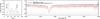 |
Fig. 1 Left panel: cross-dispersion cut showing the eight-fibre set-up. Right panel: the pipeline-reduced data provided by ESO (red) compared to our work. Below the two spectra a difference spectrum is displayed for a direct comparison of the two reductions (data taken 2009-04-03: OB ID 331412). |
Numerous searches and accurate analyses have resulted in a small sample of solar-twin candidates (Porto de Mello & da Silva 1997; Meléndez et al. 2006; Takeda et al. 2007; Meléndez et al. 2009; Ramírez et al. 2009). Although these stars in general have fundamental parameters very close to solar, recent advances in high-accuracy differential abundance analyses have proven almost all of them to have chemical compositions slightly, but systematically, deviating from that of the Sun.
A special opportunity in the search for solar twins is offered by the old and populous open cluster M67. It has a chemical composition similar to the Sun with [Fe/H] in the range −0.04 to 0.03 on the customary logarithmic scale normalised to the Sun (Hobbs & Thorburn 1991; Tautvai iene et al. 2000; Yong et al. 2005; Randich et al. 2006; Pace et al. 2008; Pasquini et al. 2008). Its age is also comparable to that of the Sun: 3.5–4.8 Gyr (e.g. Yadav et al. 2008). M67 is relatively nearby (~900 pc) and is only little affected by interstellar extinction, which allows detailed spectroscopic studies of its main-sequence stars. The depleted Li abundance of the Sun seems rather representative of solar-twins in the Galactic field (Baumann et al. 2010). M67 also seems to contain Li-depleted G stars (Pasquini et al. 1997). M67 thus offers good possibilities of finding solar-twin candidates for further exploration. Pasquini et al. (2008) (followed by a paper of Biazzo et al. 2009) recently searched the cluster for solar analogs, and listed ten promising candidates.
Here we present an analysis of M67-1194 (NGC 2682 YBP 1194, ES 4063, ES IV-63, FBC 2867, MMJ 5357, SAND 770, 2MASS J08510080+1148527), a cluster solar-twin candidate suggested by Pasquini et al. (2008). Our analysis is based on high-resolution observations with relatively high signal-to-noise (S/N) ratio. In Sect. 2, we discuss the observations and some aspects of the data reduction. Section 3 describes the analysis method and the determination of fundamental parameters (Teff, log g, [Fe/H] and ξt). In Sect. 4 we present the results of a detailed analysis of a number of chemical elements, and these results are compared to those obtained for known twins in the Galactic field. In Sect. 5, we present a new age determination for M67, and in Sect. 6 we discuss the results.
2. Observations
The observations of M67-1194 were carried out with the multi-object spectrometer FLAMES-UVES at ESO-VLT in Service Mode in the spring of 2009 during a period of three months (18th of January – 3rd of April). The observations analysed here are part of a larger project with a main goal to study atomic diffusion in stars of M67 (082.D-0726(A)). In each observing block of the project, one fibre of the spectrograph system was positioned on M67-1194 in order to collect as many observations as possible of this faint G dwarf.
We obtained altogether 18 h in 13 observing nights (23 individual observations). The spectrometer setting (RED580) was chosen to yield a resolution of R = λ/Δλ = 47 000 (1′′ fibre) and a wavelength coverage of 480–670 nm. The typical signal-to-noise ratio (S/N) per frame is 36 pixel-1 (as measured in the line-free region between 6426 Å and 6430 Å). Barycentric radial velocities were determined from the individual spectra yielding a radial velocity of −33.8 ± 0.4 km s-1. This is in exellent agreement (1σ) with the mean radial velocity of the cluster as determined by Pasquini et al. (2008), vrad = −33.30 ± 0.40, and Yadav et al. (2008), vrad = −33.673 ± 0.208. The latter study classifies M67-1194 as a high-probability proper-motion cluster member (99%). The frames were subsequently co-added for highest possible S/N ratio.
2.1. Data reduction
While ESO provides pipeline-reduced data for an initial assessment of the observed spectra, these are not intended for a full scientific analysis. In fact, we found that the extraction of our spectra by the ESO pipeline was problematic, mainly because the instrumental setup of FLAMES-UVES combined with our choice of targets is challenging. Having eight fibres tightly packed in a slit-like fashion, FLAMES-UVES can obtain echelle spectra of up to 8 targets in parallel. However, the spacing between the individual fibres is rather small, which leads to non-negligible light contamination between adjacent fibres. This was made even more challenging by the fact that our target is considerably fainter than the one of the adjacent fibre. The ESO pipeline had severe problems extracting such a spectrum, which is apparent from a strong and periodic pattern of low-sensitivity spikes. This is illustrated in Fig. 1, where we show a cross-order profile and a section of the pipeline-reduced spectrum of M67-1194 (in red) from frame OB 331412 (2009-04-03) – an illustrative frame in this context.
Given the problems in the pipeline-reduced data, we adapted the code of the echelle-reduction package REDUCE (Piskunov & Valenti 2002) to perform an accurate spectrum extraction. Here we used special calibration frames provided by ESO, the so-called even and odd flat-field frames. In these frames, only every second fibre is illuminated, which eliminates crosstalk between fibres and allows us to calculate an accurate two-dimensional model of the individual aperture shapes. The extraction of the target spectra was then performed in two steps. We first used a very narrow aperture to extract the central (non-overlapping) part of each fibre. This allowed us to estimate the relative contribution of each individual fibre at each wavelength, which we then combined with the earlier determined aperture shapes to create a full two-dimensional model (which includes spectral features) for each fibre in the observed frame. We then eliminated the fibre-to-fibre contamination by subtracting the models of adjacent apertures prior to a full extraction of each individual spectrum. We show an example of a spectrum extracted with this method in Fig. 1 (black). The periodic pattern of spikes has been removed successfully, and the agreement with the pipeline-reduced spectra outside the spikes is excellent.
Figure 2 shows a portion of the co-added spectrum covering the Mg ib lines. The S/N in the co-added spectrum reaches a mean of 160 pixel-1.
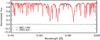 |
Fig. 2 Observations of the Mg ib triplet region, for both M67-1194 (black) and the FLAMES-UVES Sun (red). A difference spectrum is plotted below. |
3. Analysis
We performed a line-by-line differential analysis of the combined spectrum of M67-1194 relative to the Sun. The latter was represented by a day-time spectrum of the sky taken with the 580 nm setting of FLAMES-UVES in 2004 (Program ID 60.A-9022). The S/N of the solar spectrum is generally higher than that of M67-1194 (typically 230 pixel-1). Together with the Kitt-Peak Solar Atlas (Kurucz et al. 1984), this made it possible to identify blends of weak lines, in the wings of the lines measured as well as their surrounding regions used for setting the continuum.
For analysis we used SIU (Reetz 1991), a tool to visualize and compare observed and theoretical spectra. SIU has a built-in line-synthesis module which uses one-dimensional hydrostatic model atmospheres in LTE with an ODF representation of line opacity (MAFAGS, Fuhrmann et al. 1997; Grupp 2004). The line-formation code also assumes LTE. The highly differential character of the analysis make our results very little dependent on the model atmospheres used; if, e.g., the more detailed MARCS models (Gustafsson et al. 2008) were used, the same results would be obtained.
In a first step, we analysed the solar spectrum. We selected iron lines from the work of Korn et al. (2003), complemented by lines used by Meléndez et al. (2009, priv. comm.) to cover a wide range in excitation energies. The KPNO solar atlas was consulted when setting the local continuum around lines of interest. With Teff = 5777 K, log g = 4.44, [Fe/H] = 0.00, a solar microturbulence of ξt = 0.95 km s-1 was found to minimize trends of abundance with line strength for both Fe i and Fe ii.
The derivation of a differential elemental abundance is a three-step process. First, the spectral region around every spectral line of interest is carefully normalized by comparing the relative fluxes in the solar and the stellar spectrum. Next, the solar spectrum is analysed varying the product of the elemental abundance and the gf value until a satisfactory fit to the line profile is achieved. For strong lines damping parameters are based on quantum-mechanical calculations and adopted from VALD (Kupka et al. 1999). The Mg ib triplet line, used in the determination of the surface gravity, is fitted to the solar line varying the damping. The treatment of Hα follows Korn et al. (2003). The “external” profile, including effects of macroturbulence, projected rotational velocity and instrumental profile, is assumed to be Gaussian with a width determined in this fitting process. Finally, the stellar spectrum is analysed and the abundance difference noted. Steps 2 and 3 are not carried out one after the other, to avoid biases that interactive differential line fitting may be subject to. Rather, a set of lines is analysed in the solar spectrum, then the same set of lines in the stellar one, without preconceptions as regards the abundance.
We performed several test calculations to quantify to which extent this interactive procedure gives results in agreement with those of a fully automatic procedure. An unweighted χ2 on the whole line profile was found to give somewhat higher abundances in the analysis of the stellar spectrum. This is not surprising, as the experienced spectroscopist will tend to compensate for suspected blends while χ2 will blindly fit them as part of the line profile. The 1σ offset in abundance when comparing the two methods was found to be 0.01 dex. Given the good agreement between these two fitting techniques, we are confident that the results of this study are independent of the line-fitting method used. To further check our procedures, we measured equivalent widths for all spectral lines, both in the spectrum of M67-1194 and in the solar spectrum (see Tables A.1, A.2 and Fig. A.1), and analysed these widths with a fully independent set of programs (MARCS, Gustafsson et al. 2008, for the model atmospheres and the Uppsala EQWIDTH/BSYN package to calculate model spectra and equivalent widths). The departures in differential abundances | [X/Fe](M67-1194 – Sun) | were typically ± 0.01 dex or less; the maximum deviation was 0.02 dex.
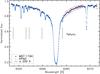 |
Fig. 3 The Hα line observed in the solar spectrum (Kitt Peak National Observatory, KPNO) and in the spectrum of M67-1194. Synthetic spectra with effective temperatures offset by ± 200 K are shown as solid lines. The most prominent telluric lines are marked out as vertical lines. |
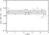 |
Fig. 4 The line-by-line difference in Fe i abundance plotted as a function of the excitation energy of each line. A slope insignificantly different from zero is found, suggesting an effective temperature close to 5780 K. The standard deviation is indicated by the grey-shaded area. |
3.1. Fundamental stellar parameters and chemical composition
The stellar parameters of M67-1194 have been constrained employing several spectroscopic techniques. The primary method to estimate the effective temperature is based on the self-broadened wings of Hα. As Fig. 3 shows, the agreement between the Hα profile observed for M67-1194 and that of the Kitt Peak atlas is excellent. Within the noise level, there are no appreciable departures, except for the few telluric lines present in our observations. The estimated effective temperature of M67-1194 when based on the wings of Hα is 5780 ± 50 K.
We furthermore analysed the excitation equilibrium of neutral iron (see Fig. 4) and obtained a Teff equal to 5780 K, omitting one uncertain high-excitation line. We derived a mean metallicity for M67-1194 of [Fe/H]I = 0.023 ± 0.015 (1σ). The uncertainty in [Fe/H] translates into an uncertainty in effective temperature at the 20 K level (1σ).
Combining the above two indicators, we adopt 5780 ± 27 K as our current best estimate of the effective temperature of M67-1194. The error is the combined error from the two methods propagated into the mean.
Since the effective temperature is of key significance for the abundance results to be discussed below, we have performed two independent checks. One is to apply the line-ratio method of Gray (1994). Here, the central line depths of two neighbouring spectral lines, one at low and one at relatively high excitation, are compared. Following Gray, we have chosen the V i 6251.8 Å line (χ = 0.29 eV) and the Fe i 6252.6 Å line (χ = 2.40 eV) and measured the ratios between their line depths in our spectra. The difference in the line-depth ratio r = d(6251.8)/d(6252.6) between M67-1194 and the Sun is found to be δr = 0.02 ± 0.02, the latter figure denoting estimated maximum errors. With the r − Teff relation of Gray (1994, Table 4) this suggests a range of Teff(M67-1194) − Teff( ⊙ ) = 60 ± 60 K, assuming a solar [V/Fe] (consistent with the results of our analysis).
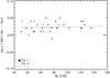 |
Fig. 5 The line-by-line difference in Fe i and Fe ii abundances plotted as a function of the equivalent width of the lines. Fe i lines return a slightly positive dependence (solid line), Fe ii (dashed line) a slightly negative one suggesting an average ξt very close to the solar value of 0.95 km s-1. |
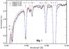 |
Fig. 6 Observations of the gravity-sensitive wing of Mg i 5183.6 Å shown together with synthetic spectra for models with log g values of 4.24, 4.44, and 4.64 (cgs units). |
A second method is to use the observed colour of the star. According to Yadav et al. (2008), (B − V)M67 − 1194 = 0.667 ± 0.01. Together with the comprehensive assessment of the reddening towards M67 (E(B − V) = 0.041 ± 0.004, Taylor 2007), this points towards a (B − V) of 0.626 ± 0.011 which is in the lower end of the interval (B − V)⊙ = 0.62 − 0.65 suggested for the Sun by contemporary studies (see Holmberg et al. 2006, who, however, favour a high value around 0.64). If we adopt the recent calibration of (B − V)(Teff) by Casagrande et al. (2010) we get Teff(M67-1194) = 5832 K. If we adopt a stellar K magnitude from the 2MASS catalogue we find (V − K) = 1.664, correct for reddening following Cox (2000) which suggests (V − K)0 = 1.556, and apply the Casagrande et al. (V − K) calibration we obtain Teff(M67-1194) = 5773 K. Taking uncertainties in continuum positioning for the line-depth estimates and reddening for the colour estimates into consideration, all these results are consistent with our adopted value of 5780 K. The line-depth ratio method and photometry suggest that this value might rather be slightly underestimated than overestimated.
The surface gravity is set by requiring lines of Fe ii to return the same differential abundance as lines of Fe i (LTE ionization equilibrium). As in the case of Fe i, we opted for a careful selection of relatively few well-observed weakly blended lines. Figure 5 demonstrates that the ionization equilibrium is established at log g = 4.44. Given the 1σ scatter among the log g-sensitive Fe ii lines (0.013 dex), the value of the surface gravity is uncertain at the 0.04 dex level. In this step, the microturbulence is found to be ξt = 0.95 km s-1 (cf. Fig. 5), i.e. the same value as used in the analysis of the solar spectrum.
Further evidence as regards the solar-like surface gravity is obtained from the analysis of the damping wings of the Mg ib lines. The Mg abundance was derived from the Mg i doublet lines at 6718.7 and 6319.2 Å which are on the linear part of the curve of growth, as well as from the moderately strong Mg i 5711 Å line. These lines consistently give the result [Mg/Fe] = 0.02 ± 0.01. There are no other suitable atomic Mg lines in the spectral regions available to us. To get further constraints on the Mg abundance, we explored the wavelength region around 5134–5137 Å with Q2(23), Q1(23) and R2(11) features of the (0,0) bands of the A-X system of MgH. This region is severely affected also by lines from the C2 Swan bands. The observed spectrum appears very similar but with about 8% stronger MgH bands, as compared with the solar spectrum. Our spectrum synthesis, assuming solar isotopic ratios, shows that the observed MgH bands are consistent with our abundance estimate for Mg and the somewhat enhanced overall metallicity. The adoption of a significantly lower Mg abundance (by 0.1 dex) would, lead to too weak MgH features. Adopting [Mg/H] = 0.02, the pressure-broadened red wing of Mg i 5183 Å (the strongest line of the Mg i triplet with the largest log g sensitivity) indicates a log g of 4.44 ± 0.05 (see Fig. 6). To this we add in quadrature the uncertainty stemming from the Mg abundance. This yields an error for log g of 0.06.
Combining the two independent methods (Fe i/ii, Mg ib), we finally adopt 4.44 ± 0.035 as our current best estimate of the surface gravity of M67-1194. The error is the combined error from the two methods, propagated into the mean.
Abundances are determined using the line list of Meléndez et al. (2009), which was chosen in order to make our results directly comparable to the twin results of that group. In the case of carbon, we needed to depart from that list replacing lines not available in our wavelength range with C2 lines. In the case of oxygen, inspection of the wavelength regions around the [O i] lines at 6300.3 and 6363.7 Å proved this region to be far too noisy for an accurate oxygen abundance determination. Within this noise, the spectrum does not depart significantly from the solar spectrum, and fits of synthetic spectra suggest the oxygen abundance ratio [O/Fe] to be solar with an estimated maximum error of about 0.15 dex. The high excitation O i 6158.1 line was found to be more useful at this level of S/N, allowing an estimated [O/Fe] = 0.07 ± 0.07. These errors are here to be seen as maximum errors, and the uncertainties are mainly related to the placement of the continuum. We note that this result is consistent with the mean [O/Fe] = 0.01 ± 0.03, as determined for ten somewhat brighter and hotter main-sequence stars in M67 by Randich et al. (2006) using the 6300.3 Å line.
The resulting abundances are illustrated in Fig. 7 as differences between the solar values and those of M67-1194, and compared to the mean results for the solar twin sample of Meléndez et al. (2009). We note that, given the similarity of the spectrum of M67-1194 to the solar one, uncertainties in line data effectively cancel. Similarly, errors due to inadequacies in the model atmospheres, e.g., in describing the formation of molecular lines in the upper layers of the atmospheres, should cancel, provided that the elemental abundances are practically the same, and no other effects but those related to the fundamental stellar parameters characterize the atmospheres.
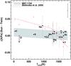 |
Fig. 7 Abundance difference as a function of condensation temperature (according to Lodders 2003). Filled circles: this paper, plus signs: Meléndez et al. (2009). Shaded area: this paper, dotted line: Meléndez et al. (2009). The shaded area summarizes the result of this paper when submitted to a linear-regression analysis (including the upper limit of O), giving Δ [X/Fe] = a + mTcond. The area delineates the range of regression lines due to the uncertainties in a and m. The elements in the range 1300–1500 K not identified are (from left to right): Cr, Si, Co, Ni and V. Error bars are discussed in detail in Sect. 3.2. |
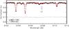 |
Fig. 8 M67-1194 compared to the FLAMES-UVES spectrum representing the Sun (red). The difference spectrum is shown below (offset by +0.7 units). At the current S/N level, there is no systematic difference between the two spectra at the position of the Li i doublet. |
3.2. Abundance errors
There are several kinds of errors that could have an impact on our abundance results. Despite the good data quality achieved for this faint star, continuum placement is a non-negligible source of error (see the case of oxygen above and lithium below). However, it can be classified as a random error, given the similarity between the solar and the stellar spectrum and the differential nature of our analysis. Thus, these errors are reflected in the line-to-line scatter in abundances. Errors stemming from stellar-parameter uncertainties are also discussed below.
The error bars indicated in Fig. 7 are the sample standard deviation for the abundance of each element as determined from the available lines, e.g. they represent internal errors. Given the generally small number of lines, we adopt this more conservative estimate over the standard deviation of the mean (as throughout this study). If this error is found to be below 0.02 dex, we adopt 0.02 dex as a lower limit (indicated in the upper right corner of Fig. 7 and representative of all points without error bars). In the case of Na (two lines giving abundances in numerical agreement) we adopted an estimate of the fitting error.
The result shown in Fig. 7 could also be affected by errors in fundamental parameters of M67-1194. Generally, errors in fundamental stellar parameters would lead to vertical shifts of the points by typically 0.00–0.02 dex. Exploring this in detail, we have found that the only error which could qualitatively affect the abundance trend would be an overestimate of the effective temperature by 50 K or more. If the star were cooler by that amount, the abundances of the volatiles would be overestimated so that when correcting for that error the points for C, O and S in the diagram would be pushed upwards towards the red dashed Meléndez twin line while some points representing refractories in the right part of the diagram would be pushed down. In view of the discussion of possible errors and biases in Teff (M67-1194) we find, however, such an overestimate improbable.
4. M67-1194 in comparison with other twins
The resulting abundance ratios for M67-1194 relative to iron and normalized on the solar abundances, are plotted in Fig. 7 versus the 50% condensation temperature of the various elements, according to Lodders (2003). Here, the results of Meléndez et al. (2009) for their sample of eleven solar twins in the Galactic field are also indicated, and following those authors we plot the differences between the solar abundances and corresponding stellar results.
Meléndez et al. found that for almost all their stars, the volatile elements are relatively less abundant than in the Sun, while the refractory elements are somewhat enhanced in the stars. This effect is seemingly not present in the M67 twin, at least not to the same extent. It is thus seen (cf. Fig. 7) that the abundance profile of M67-1194 is more similar to the Sun than for all the Meléndez et al. twins, with one or two exceptions. We perform a simple statistical test, essentially judging the probability that all black dots in Fig. 7 just by chance fall above the red dashed line for Tcond > 1400 K, and below it for Tcond < 1400 K. We find that the probability for M67-1194 to be drawn from the same sample of stars as the majority of the Meléndez et al. twins is less than 5%. On the other hand, the errors in the analysis are fully compatible with solar abundance ratios for the M67 star. This astonishing result will be discussed further below.
4.1. Lithium content
Pasquini et al. (2008) estimated the lithium content of ten solar-type stars in M67 including M67-1194 from FLAMES-MEDUSA data. The authors derived lithium abundances similar to that of the Sun from the Li doublet at 6707.8 Å, using spectra with a resolution of R ~ 17 000 and a S/N ratio of 80–110 pixel-1. The weakness of the Li i 6707.8 Å doublet in M67-1194 and the noise level of the spectra make it difficult to determine an accurate Li abundance for the twin. A major problem is the location of the local continuum around the line. With our preferred positioning of the continuum (cf. Fig. 9, lower part) we find a stronger 6707 Å line than the solar one, and a Li abundance of log ε = 1.26, corresponding to [Li/H] = +0.2 dex. This continuum positioning presumes that the wide depression around 6707.8 Å is a real spectral feature, and not due to some instrumental effect. If the latter is assumed, a more local continuum drawing is appropriate (see upper part of Fig. 9). This would lead to a Li abundance close to solar, [Li/H] = 0.0, i.e. a value closer but still greater than that obtained by Pasquini et al. (2008), [Li/H] < –0.2. We regard the Li i doublet line identification in M67-1194 to be a probable but not a definitive one. It can therefore not be excluded that the true abundance is significantly below solar. Probably, however, the Li abundance of M67-1194 is solar or larger, but not exceeding the solar value by more than a factor of 2.5.
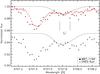 |
Fig. 9 Upper part: the spectrum of M67-1194 (black bullets) around Li i 6707 Å with a local continuum compared to the FLAMES-UVES spectrum representing the Sun (red circles). The best theoretical fit to the spectrum is shown as a solid line. Lower part: a global continuum placement for M67-1194 together with the best theoretical fit (both offset vertically by 0.045 units). |
5. The age of M67
Analysing a target very similar to the Sun, we profit from a number of advantages. The spectroscopic stellar parameters are more accurately determined than is generally achieved. This is again a result of the strictly differential approach relative to the Sun, which is expected to promote cancellation of the modelling errors that usually dominate these types of analyses. The absolute accuracy in the values obtained is directly based on the accurate knowledge of the solar parameters.
The age determination also benefits from these advantages of a differential approach. The stellar-evolutionary tracks are admittedly uncertain, due to e.g. diffusion, mixing and overshooting, the choice of mixing length parameter (α) and He mass fraction (Y), as well as the absolute values of the solar CNO abundances. However, α and Y are set to fit the solar radius and age. Assuming that α and Y are close to solar also for the solar twin, we may then use the tracks calibrated in this way to obtain the age of the twin and thus of M67.
Using the current version of the Victoria stellar evolutionary code, we have computed several grids of tracks in order to evaluate the dependence of the predicted age on Teff, log g, Y and [Fe/H]. The main improvements that have been made to this code since the VandenBerg et al. (2007) study of M67 are the following: (1) The gravitational settling of helium and turbulent mixing that occur below the envelope convection zones are now treated, using methods very similar to those employed by Proffitt & Michaud (1991)1, (2) the latest rates for H-burning reactions (see Weiss 2008; Marta et al. 2008) and the improved conductive opacities given by Cassisi et al. (2007) have been adopted and (3) the assumed solar abundances are those reported by Asplund et al. (2009). To reproduce the properties of the Sun at its present age (4.57 Gyr; Bahcall et al. 2005), it is necessary to adopt an initial helium content corresponding to Y = 0.2553, along with a value of αMLT = 2.007 for the usual mixing-length parameter.The evolutionary tracks in each grid, for masses in the range 0.98 ≤ ℳ/ℳ⊙ ≤ 1.06, were evolved from fully-convective structures high on the Hayashi line to the solar age. Interpolations between the tracks yielded values of Teff and log g at ages ranging from 3.5 to 4.57 Gyr, which encompasses most of the ages that have been determined for M67 in the past decade (see below). An example of one of the computed grids on the (Teff, log g)-plane is shown in Fig. 10.
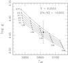 |
Fig. 10 Plot of the 3.5 to 4.57 Gyr segments of the post-main-sequence tracks (dashed) that were computed for masses from 0.98 to 1.06 ℳ⊙ (indicated below each track) and the indicated values of Y and [Fe/H]. Open circles represent the Teff and log g values at the ages noted just to the right of the y-axis; and hence the solid curves are isochrones for those ages. The filled circle and attached error bars indicate the location of the solar twin, M67-1194. |
The chemical-composition dependence of the inferred mass and age of M67-1194.
From cubic spline interpolations in these results, the inferred age of the solar twin is 4.21 Gyr and its mass is estimated to be 1.013 ℳ⊙. At Teff = 5780 K, one can readily determine that the gravity uncertainty implies a range in age from ≈2.6 to 5.6 Gyr. The age range spanned by the Teff error bar is much smaller, 3.8–4.6 Gyr. Similar analyses of the model grids which were computed for slightly different helium and metal abundances yield the results that are listed in Table 1. The measured uncertainty in [Fe/H] (±.015) implies an age uncertainty of approximately ±0.2 Gyr, whereas the evolutionary calculations predict about a ± 0.3 Gyr change in age if the assumed value of Y is altered by ± 0.01. Meléndez et al. (2009) propose that the Sun could have a reduced fraction of refractories in its present relatively thin convection zone, as compared with the composition of its interior. The effects of such a chemical inhomogeneity not only for the Sun but also for M67-1194 on its age determination would cancel, but it is also possible that the twin, in spite of its solar abundance profile in the atmosphere, does not have a corresponding inhomogeneity. In that case, we find (using the results given in the bottom row of Table 1) a systematic error in the age determination, leading to an underestimate of the age by about 0.35 Gyr. Table 2 provides a convenient summary of the errors in the fundamental parameters of M67-1194 and their effects on its inferred mass and age.
Our best estimate of the age of M67-1194 (4.2 ± 1.6 Gyr) agrees very well with determinations based on alternative methods. Most fits of isochrones to the M67 color-magnitude diagram, whether using Garching (see Magic et al. 2010), Montreal (Michaud et al. 2004), Padova (Yadav et al. 2008), Teramo (Bellini et al. 2010), Victoria (VandenBerg et al. 2007), or Yale-Yonsei (Yadav et al.) isochrones, favour an age of 4.0 ± 0.3 Gyr. Moreover, Bellini et al. have recently found that the age obtained from the cluster white dwarfs is fully consistent with the aforementioned turnoff age. However, higher ages cannot yet be completely excluded (see examples provided by Yadav et al. and Magic et al.). We note that the solar age is within the 2σ error bar of M67’s age.
Errors (ϵ) in mass and age estimates for M67-1194 due to uncertainties in fundamental stellar parameters.
6. Discussion
Our main finding, illustrated in Fig. 7, is that M67-1194 is indeed more similar to the Sun than most of the nearby solar twins in the field. This is interesting in view of the possible explanations for the systematic departures of the field twin from the Sun in abundances with condensation temperature, found and discussed by Meléndez et al. (2009, see also Gustafsson et al. 2010). Basically, three possible explanations were discussed: (1) The solar proto-planetary gas disk was sufficiently long-lived, after the gas had been depleted in refractories by the formation of planetesimals and planets, for the solar convection zone to become so thin that the accreted gas could give visible traces in the solar spectrum. The field twins, however, in general accreted their gas disks much earlier. (2) The solar outer convection zone never reached deep enough to encompass most of the solar mass, and was therefore much more easily polluted by the rarified infalling disk. This property of the Sun, presumably reflecting the initial conditions of the cloud to later form the Sun and the Solar System or the details of the more or less episodic accretion history of the Sun (cf. Baraffe & Chabrier 2010), was not usual among solar-type stars and is thus not shared by most twins. (3) The proto-solar cloud was cleansed by radiation fields from massive stars, pushing dust grains out of the cloud. These effects must then have been greater for the solar cloud than for most of the twins.
If the tendency found here for our M67 twin is representative for the cluster, it speaks against the first explanation above. We see no reason why the gas disks around stars in a cluster should have longer life-times than those in the field. It might be that the initial conditions of star formation are different in a cluster than in the field, and that this might couple to the evolution of the stellar convection zones, but this is only speculation. Maybe, a more episodic accretion history, gradually building stars from quite small entities, is more characteristic of a cluster environment. In any case, there is independent evidence from radioisotopic abundances in the solar system that the Sun was born in a cluster (Looney et al. 2006; see also Portegies Zwart 2009) containing relatively close supernovae or massive AGB stars (Trigo-Rodríguez et al. 2009).
The similarity of the age and overall composition of the Sun with the corresponding data of M67, and in particular the agreement of the detailed chemical composition of the Sun with that of M67-1194, could suggest that the Sun has formed in this very cluster. According to the numerical simulations by Hurley et al. (2005) the cluster has lost more than 80% of its stars by tidal interaction with the Galaxy, in particular when passing through the Galactic plane, and the Sun might be one of those. We note that the orbit of the cluster encloses, within its apocentre and pericentre, the solar orbit. However, the cluster has an orbit extending to much higher Galactic latitudes, presently it is close to its vertical apex at z = 0.41 kpc (Davenport & Sandquist 2010), while the Sun does not reach beyond z = 80 pc (Innanen et al. 1978). Thus, in order for this hypothesis of an M67 origin of the Sun to be valid, it must have been dispersed from the cluster into an orbit precisely in the plane of the Galactic disk, which seems improbable.
7. Conclusions
We draw the following conclusions from the analysis of M67-1194 presented here:
-
Within the framework of a differential analysis, the stellar parameters (Teff, log g, mass and age) of M67-1194 are found to be compatible with the solar values, while [Fe/H] is found to be slightly super-solar. M67-1194 is thus the first solar twin known to belong to a stellar association.
-
The chemical abundance pattern of M67-1194 closely resembles the solar one, in contrast to most known solar twins. This suggests similarities in the formation of M67-1194 and the Sun. A common origin of both stars as members of M67 is conceivable, albeit not likely, considering their different Galactic orbits. If the chemical abundance pattern reflects environmental effects, then the Sun was likely born in a cluster similar to M672.
-
Of the three scenarios for the peculiar abundance pattern of the Sun relative to field solar twins presented in Meléndez et al. (2009), a particularly long-lived gas disk is the least probable due to the cluster membership of M67-1194. In the standard picture of stellar evolution with an early fully-convective phase, dust cleansing by nearby luminous stars seems to have affected both the Sun and M67-1194. Another possibility is that the initial boundary conditions or accretion history of the early Sun were similar to those in the young cluster, and that these led to a shallow convection zone in the early evolution of these stars. More stars in M67 must be investigated to give further support to such explanations.
Methodologically, we consider the method of age determination, based on spectroscopy of solar-like stars, to be an interesting alternative to other determinations of cluster ages (as independently done by Castro et al. 2011). Its main advantages is that the uncertainties in cluster distance and reddening are not important. The age errors, in particular due to errors in the surface gravity, could be further reduced by higher S/N, a wider spectral range and observations of more stars. The uncertainty due to the unknown He abundance could be reduced by accurate studies of the horizontal branch or of visual binaries. In fact, the method can be extended to age estimates for other clusters, including globular ones. The basic idea is to make a systematic spectroscopic comparison with well known standard stars with very similar parameters in the nearby field or in other clusters. Even if the absolute ages of these standards are not as well established, the method offers an accurate age ranking, revealing possible age differences between different populations of clusters.
In general, the highly differential method used here has great possibilities in other situations when detailed comparisons are to be carried out e.g. between Thick and Thin Galactic-disk stars, or different types of Halo stars. Then, a close adherence to a pairwise selection of stars with similar effective temperatures and metallicities will make it possible to keep the systematic modelling errors at a low level.
Online material
Appendix A: Chemical elements
Fe i and Fe ii lines used in the analysis.
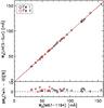 |
Fig. A.1 Upper panel: comparison of equivalent widths of M67-1194 and the FLAMES/UVES sky spectrum representing the Sun. 1D polynomial fits for both Fe i and Fe ii are shown as solid and dashed lines, respectively. Lower panel: the percentage equivalent-width difference of Fe i and Fe ii lines between M67-1194 and the FLAMES/UVES sky spectrum representing the Sun. Note that the abundances are not derived from equivalent widths, but from fits of synthetic spectra. |
Chemical elements (except Fe) and spectral lines in the analysis.
At the solar age, settling reduces the surface helium abundance to Y = 0.2384, which is slightly less than the value inferred from helioseismology, but similar to the values predicted by other Standard Solar Models, see the Bahcall et al. paper. Following Proffitt and Michaud, the free parameter in the adopted treatment of turbulent mixing was set so that our model for the Sun predicts the observed solar Li abundance.
Acknowledgments
We thank the anonymous referee whose constructive criticism considerably improved the paper. A.Ö. acknowledges support by Värmlands nation (Uddeholms research scholarship). A.J.K. acknowledges support by the Swedish Research Council and the Swedish National Space Board.
References
- Asplund, M., Grevesse, N., Sauval, A. J., & Scott, P. 2009, ARA&A, 47, 481 [NASA ADS] [CrossRef] [Google Scholar]
- Bahcall, J. N., Basu, S., Pinsonneault, M., & Serenelli, A. M. 2005, ApJ, 618, 1049 [NASA ADS] [CrossRef] [Google Scholar]
- Baraffe, I., & Chabrier, G. 2010, A&A, 521, A44 [NASA ADS] [CrossRef] [EDP Sciences] [Google Scholar]
- Baumann, P., Ramírez, I., Meléndez, J., Asplund, M., & Lind, K. 2010, A&A, 519, A87 [NASA ADS] [CrossRef] [EDP Sciences] [Google Scholar]
- Biazzo, K., Pasquini, L., Bonifacio, P., Randich, S., & Bedin, L. R. 2009, MmSAI, 80, 125 [Google Scholar]
- Bellini, A., Bedin, L. R., Piotto, G., et al. 2010, A&A, 513, A50 [NASA ADS] [CrossRef] [EDP Sciences] [Google Scholar]
- Casagrande, L., Ramírez, I., Meléndez, J., Bessell, M., & Asplund, M. 2010, A&A, 512, 54 [Google Scholar]
- Cassisi, S., Potekhin, A., Pietrinferni, A., Catelan, M., & Salaris, M. 2007, ApJ, 661, 1094 [NASA ADS] [CrossRef] [Google Scholar]
- Castro, M., do Nascimento Jr., J. D., Biazzo, K., Meléndez, J., & De Medeiros, J. R. 2011, A&A, 526, A17 [NASA ADS] [CrossRef] [EDP Sciences] [Google Scholar]
- Cayrel de Strobel, G. 1996, A&ARv, 7, 243 [CrossRef] [Google Scholar]
- Cayrel de Strobel, G., Knowles, N., Hernandez, G., & Bentolila, C. 1981, A&A, 94, 1 [NASA ADS] [Google Scholar]
- Cox, A. N. 2000, Allen’s Astrophysical Quantities, 4th edn. (New York: Springer-Verlag, Inc.) [Google Scholar]
- Davenport, J. R. A., & Sandquist, E. L. 2010, ApJ, 711, 559 [NASA ADS] [CrossRef] [Google Scholar]
- Fuhrmann, K., Pfeiffer, M., Frank, C., Reetz, J., & Gehren, T. 1997, A&A, 323, 909 [NASA ADS] [Google Scholar]
- Gray, D. F. 1994, PASP, 106, 1248 [NASA ADS] [CrossRef] [Google Scholar]
- Grupp, F. 2004, A&A, 420, 289 [NASA ADS] [CrossRef] [EDP Sciences] [Google Scholar]
- Gustafsson, B. 1998, SSrv, 85, 419 [Google Scholar]
- Gustafsson, B., Edvardsson, B., Eriksson, K., et al. 2008, A&A, 486, 951 [NASA ADS] [CrossRef] [EDP Sciences] [Google Scholar]
- Gustafsson, B., Meléndez, J., Asplund, M., & Yong, D. 2010, Ap&SS, 328, 185 [NASA ADS] [CrossRef] [Google Scholar]
- Hardorp, J. 1978, A&A, 63, 383 [NASA ADS] [Google Scholar]
- Hobbs, L. M., & Thorburn, J. A. 1991, AJ, 102, 1070 [NASA ADS] [CrossRef] [Google Scholar]
- Holmberg, J., Flynn, C., & Portinari, L. 2006, MNRAS, 367, 449 [NASA ADS] [CrossRef] [Google Scholar]
- Hurley, J. R., Pols, O. R., Aarseth, S. J., & Tout, C. A. 2005, MNRAS, 363, 293 [NASA ADS] [CrossRef] [Google Scholar]
- Innanen, K. A., Patrick, A. T., & Duley, W. W. 1978, Ap&SS, 57, 511 [NASA ADS] [CrossRef] [Google Scholar]
- Korn, A. J., Shi, J., & Gehren, T. 2003, A&A, 407, 691 [NASA ADS] [CrossRef] [EDP Sciences] [Google Scholar]
- Kraft, R. P., Sneden, C., Smith, G. H., et al. 2007, AJ, 113, 279 [Google Scholar]
- Kurucz, R. L., Furenlid, I., Brault, J., & Testerman, L. 1984, Solar Flux Atlas from 296 to 1300 nm, Kitt Peak National Solar Observatory [Google Scholar]
- Lodders, K. 2003, ApJ, 591, 1220 [NASA ADS] [CrossRef] [Google Scholar]
- Looney, L. W., Tobin, J. J., & Fields, B. D. 2006, 652, 1755 [Google Scholar]
- Magic, Z., Serenelli, A. M., Weiss, A., & Chaboyer, B. 2010, ApJ, 718, 1378 [NASA ADS] [CrossRef] [Google Scholar]
- Marta, M., formicola, A., Gyürky, G. Y., et al. 2008, Phys. Rev. C, 78, 022802 [NASA ADS] [CrossRef] [Google Scholar]
- Meléndez, J., & Ramírez, I. 2007, ApJ, 669, 89 [Google Scholar]
- Meléndez, J., Dodds-Eden, K., & Robles, J. 2006, ApJ, 641, 133 [NASA ADS] [CrossRef] [Google Scholar]
- Meléndez, J., Asplund, M., Gustafsson, B., & Yong, D. 2009, ApJ, 704, L66 [NASA ADS] [CrossRef] [Google Scholar]
- Michaud, G., Richard, O., Richer, J., & VandenBerg, D. A. 2004, ApJ, 606, 452 [NASA ADS] [CrossRef] [EDP Sciences] [Google Scholar]
- Pace, G., Pasquini, L., & François, P. 2008, A&A, 489, 403 [NASA ADS] [CrossRef] [EDP Sciences] [Google Scholar]
- Pasquini, L., Randich, S., & Pallavicini, R. 1997, A&A, 325, 535 [NASA ADS] [Google Scholar]
- Pasquini, L. Biazzo, K., Bonifacio, P., Randich, S., & Bedin, L. R. 2008, A&A, 489, 677 [NASA ADS] [CrossRef] [EDP Sciences] [Google Scholar]
- Piskunov, N. E., & Valenti J. A. 2002, A&A 385, 1095 [Google Scholar]
- Portegies Zwart, S. F. 2009, ApJ, 696, 13 [Google Scholar]
- Porto de Mello, G. F., & da Silva, L. 1997, ApJ, 482, 89 [Google Scholar]
- Porto de Mello, G. F., da Silva, R., & da Silva, L. 2000, ASPC, 213, 73 [NASA ADS] [Google Scholar]
- Ramírez, I., Meléndez, J., & Asplund, M. 2009, A&A, 508, 17 [NASA ADS] [CrossRef] [EDP Sciences] [Google Scholar]
- Proffitt, C. R., & Michaud, G. 1991, ApJ, 371, 584 [NASA ADS] [CrossRef] [Google Scholar]
- Randich, S., Sestito, P., Primas, F., Pallavicini, R., & Pasquini, L. 2006, A&A, 450, 557 [NASA ADS] [CrossRef] [EDP Sciences] [Google Scholar]
- Reetz, J. K. 1991, Diploma Thesis, Universität München [Google Scholar]
- Takeda, Y., Kawanomoto, S., Honda, S., Ando, H., & Sakurai, T. 2007, A&A, 468, 663 [NASA ADS] [CrossRef] [EDP Sciences] [Google Scholar]
- Taylor, B. J. 2007, AJ, 133, 370 [NASA ADS] [CrossRef] [Google Scholar]
- Tautvaišiene, G., Edvardsson, B., Tuominen, I., & Ilyin, I. 2000, A&A, 360, 499 [NASA ADS] [Google Scholar]
- Trigo-Rodríguez, J. M., García-Hernández, D. A., Lugaro, M., et al. 2009, M&PS, 44, 627 [Google Scholar]
- VandenBerg, D. A., Gustafsson, B., Edvardsson, B., Eriksson, K., & Ferguson, J. 2007, ApJ, 666, 105 [Google Scholar]
- Weiss, A. 2008, Phys. Scripta T, 133, 014025 [Google Scholar]
- Yadav, R. K. S., Bedin, L. R., Piotto, G., et al. 2008, A&A, 484, 609 [NASA ADS] [CrossRef] [EDP Sciences] [Google Scholar]
- Yong, D., Carney, B. W., & Teixera de Almeida, M. L. 2005, AJ, 130, 597 [NASA ADS] [CrossRef] [Google Scholar]
All Tables
Errors (ϵ) in mass and age estimates for M67-1194 due to uncertainties in fundamental stellar parameters.
All Figures
|
Fig. 1 Left panel: cross-dispersion cut showing the eight-fibre set-up. Right panel: the pipeline-reduced data provided by ESO (red) compared to our work. Below the two spectra a difference spectrum is displayed for a direct comparison of the two reductions (data taken 2009-04-03: OB ID 331412). |
| In the text | |
|
Fig. 2 Observations of the Mg ib triplet region, for both M67-1194 (black) and the FLAMES-UVES Sun (red). A difference spectrum is plotted below. |
| In the text | |
|
Fig. 3 The Hα line observed in the solar spectrum (Kitt Peak National Observatory, KPNO) and in the spectrum of M67-1194. Synthetic spectra with effective temperatures offset by ± 200 K are shown as solid lines. The most prominent telluric lines are marked out as vertical lines. |
| In the text | |
|
Fig. 4 The line-by-line difference in Fe i abundance plotted as a function of the excitation energy of each line. A slope insignificantly different from zero is found, suggesting an effective temperature close to 5780 K. The standard deviation is indicated by the grey-shaded area. |
| In the text | |
|
Fig. 5 The line-by-line difference in Fe i and Fe ii abundances plotted as a function of the equivalent width of the lines. Fe i lines return a slightly positive dependence (solid line), Fe ii (dashed line) a slightly negative one suggesting an average ξt very close to the solar value of 0.95 km s-1. |
| In the text | |
|
Fig. 6 Observations of the gravity-sensitive wing of Mg i 5183.6 Å shown together with synthetic spectra for models with log g values of 4.24, 4.44, and 4.64 (cgs units). |
| In the text | |
|
Fig. 7 Abundance difference as a function of condensation temperature (according to Lodders 2003). Filled circles: this paper, plus signs: Meléndez et al. (2009). Shaded area: this paper, dotted line: Meléndez et al. (2009). The shaded area summarizes the result of this paper when submitted to a linear-regression analysis (including the upper limit of O), giving Δ [X/Fe] = a + mTcond. The area delineates the range of regression lines due to the uncertainties in a and m. The elements in the range 1300–1500 K not identified are (from left to right): Cr, Si, Co, Ni and V. Error bars are discussed in detail in Sect. 3.2. |
| In the text | |
|
Fig. 8 M67-1194 compared to the FLAMES-UVES spectrum representing the Sun (red). The difference spectrum is shown below (offset by +0.7 units). At the current S/N level, there is no systematic difference between the two spectra at the position of the Li i doublet. |
| In the text | |
|
Fig. 9 Upper part: the spectrum of M67-1194 (black bullets) around Li i 6707 Å with a local continuum compared to the FLAMES-UVES spectrum representing the Sun (red circles). The best theoretical fit to the spectrum is shown as a solid line. Lower part: a global continuum placement for M67-1194 together with the best theoretical fit (both offset vertically by 0.045 units). |
| In the text | |
|
Fig. 10 Plot of the 3.5 to 4.57 Gyr segments of the post-main-sequence tracks (dashed) that were computed for masses from 0.98 to 1.06 ℳ⊙ (indicated below each track) and the indicated values of Y and [Fe/H]. Open circles represent the Teff and log g values at the ages noted just to the right of the y-axis; and hence the solid curves are isochrones for those ages. The filled circle and attached error bars indicate the location of the solar twin, M67-1194. |
| In the text | |
|
Fig. A.1 Upper panel: comparison of equivalent widths of M67-1194 and the FLAMES/UVES sky spectrum representing the Sun. 1D polynomial fits for both Fe i and Fe ii are shown as solid and dashed lines, respectively. Lower panel: the percentage equivalent-width difference of Fe i and Fe ii lines between M67-1194 and the FLAMES/UVES sky spectrum representing the Sun. Note that the abundances are not derived from equivalent widths, but from fits of synthetic spectra. |
| In the text | |
Current usage metrics show cumulative count of Article Views (full-text article views including HTML views, PDF and ePub downloads, according to the available data) and Abstracts Views on Vision4Press platform.
Data correspond to usage on the plateform after 2015. The current usage metrics is available 48-96 hours after online publication and is updated daily on week days.
Initial download of the metrics may take a while.