| Issue |
A&A
Volume 526, February 2011
|
|
|---|---|---|
| Article Number | A60 | |
| Number of page(s) | 13 | |
| Section | The Sun | |
| DOI | https://doi.org/10.1051/0004-6361/201015391 | |
| Published online | 22 December 2010 | |
Interpretation of HINODE SOT/SP asymmetric Stokes profiles observed in the quiet Sun network and internetwork
1
ESA/ESTEC RSSD, Keplerlaan 1, 2200
AG
Noordwijk,
Netherlands
e-mail: This email address is being protected from spambots. You need JavaScript enabled to view it.
2
Dipartimento di Fisica, Università degli Studi di Roma “Tor
Vergata”, via della Ricerca
Scientifica 1, 00133
Roma,
Italy
e-mail: This email address is being protected from spambots. You need JavaScript enabled to view it.
; This email address is being protected from spambots. You need JavaScript enabled to view it.
3
Instituto de Astrofísica de Canarias,
38205
La Laguna, Tenerife,
Spain
e-mail: This email address is being protected from spambots. You need JavaScript enabled to view it.
Received: 14 July 2010
Accepted: 28 September 2010
Abstract
Stokes profiles emerging from the magnetized solar photosphere and observed by SOT/SP aboard the HINODE satellite exhibit a variety of complex shapes. These are indicative of unresolved magnetic structures that have been overlooked in the inversion analyses performed so far. Here we present the first interpretation of the Stokes profile asymmetries measured in the Fe i 630 nm lines by SOT/SP, in both quiet Sun internetwork (IN) and network regions. The inversion is carried out based on the hypothesis of MIcro-Structured Magnetized Atmosphere (MISMA), where the unresolved structure is assumed to be optically thin. We analyze a 29.52″ × 31.70″ subfield carefully selected to be representative of the properties of a 302″ × 162″ quiet Sun field-of-view (FOV) at the disk center.The inversion code is able to reproduce the observed asymmetries in a very satisfactory way, including 35% of the inverted profiles with large asymmetries. The inversion code interprets 25% of inverted profiles as emerging from pixels in which both positive and negative polarities coexist. These pixels are located in either frontiers between opposite polarity patches or very quiet regions. The kG field strengths are found at the base of the photosphere in both network and IN regions; in the case of the latter, both kG fields and hG fields are admixed. When considering the magnetic properties of the mid photosphere, most kG fields do not exist, and the statistics is dominated by hG fields. According to the magnetic filling factors derived from the inversion, we constrain the magnetic field of only 4.5% of the analyzed photosphere (and this percentage reduces to 1.3% when considering all pixels, including those with low polarization that have not been analyzed). The properties of the rest of the plasma imply that weak fields do not contribute to the detected polarization signals. The average flux densities derived in the full subfield and IN regions are higher than those derived from the same dataset by Milne-Eddington (ME) inversion.We detect large asymmetries in the HINODE SOT/SP polarization profiles. These are not negligible in quiet Sun data. The MISMA inversion code reproduces them in a satisfactory way, and provides a statistical description of the magnetized IN and network which partly differs and complements the results obtained so far. The importance of having a complete interpretation of the line profile shapes is therefore clearly evident.
Key words: Sun: photosphere / Sun: surface magnetism / techniques: polarimetric
© ESO, 2010
1. Introduction
The spectropolarimeter SOT/SP (Lites et al. 2001; Tsuneta et al. 2008) aboard the Japanese HINODE satellite (Kosugi et al. 2007) combines  angular resolution and 10-3 polarimetric sensitivity to perform seeing-free full Stokes measurements of the polarized light emerging from the magnetized solar photosphere. Since its launch in 2006, the SOT/SP instrument has allowed the solar community to investigate the solar surface magnetism under unprecedented stable conditions.
HINODE SOT/SP observations have been analyzed intensely to investigate the quiet Sun magnetism. Its global properties have been described by Orozco Suárez et al. (2007a), Lites et al. (2008), Asensio Ramos (2009), and Jin et al. (2009), while detailed analyses of its local properties, which depend on the temporal evolution due to its interaction with plasma, have been carried out by Centeno et al. (2007), Orozco Suárez et al. (2008), Nagata et al. (2008), Shimizu et al. (2008), Fischer et al. (2009), and Zhang et al. (2009).
The above studies were performed exploiting inversion techniques for interpretation of the observed Stokes profiles. In most cases, the hypothesis of ME atmosphere was adopted to infer the properties of the magnetic field vector in HINODE resolution elements. It assumes that the polarization is produced in an atmosphere where the magnetic field vector is constant. This approximation is a good compromise to interpret large data sets in reasonable times, such as the ones obtained by HINODE. However, it is important to realize that HINODE angular resolution is still too low to perform spectropolarimetric observations of magnetic structures that can be regarded as uniform (e.g., Sánchez Almeida 2004; Stenflo 2009). As we emphasize in Sect. 3.1, asymmetric Stokes profiles in HINODE quiet Sun observations are the rule rather than the exception, which implies that unresolved structure is present (Sánchez Almeida et al. 1996, and references therein). The ME analyses cannot reproduce them, overlooking the expected coexistence of several magnetic components in a single resolution element1.
Sánchez Almeida et al. (1996) put forward arguments for describing the atmosphere where the polarization is formed as a MIcro-Structured Magnetic Atmosphere (MISMA), i.e., an atmosphere in which magnetic fields have structures smaller than the photon mean-free path in the solar photosphere (≲100 km). It can be regarded as a limiting case of structures of all sizes (e.g. Landi Degl’Innocenti 1994a,b). The MISMA hypothesis simplifies the radiative transfer, yet it provides realistic asymmetric Stokes profiles. On the basis of this hypothesis, the polarization from a single pixel in spectropolarimetric observations is equivalent to that produced by the average atmosphere. If one considers several components with diverse physical properties (i.e., thermodynamics, plasma motions, and magnetic fields), the resulting spectrum is not a linear combination of Stokes profiles emerging from each magnetic component. The superposition is instead non-linear, giving rise to asymmetries with the properties observed in the Sun (e.g., with spectral lines that produce net circular polarization). Sánchez Almeida & Lites (2000) illustrated how this complex scenario can be properly adapted using a three-component model MISMA, whose implementation in an inversion code (Sánchez Almeida 1997) allowed them to reproduce the full variety of profile asymmetries emerging from the quiet Sun when observed with the instrumentation available at the time. Stokes profiles in IN and network observations performed with HINODE contain important asymmetries, which encouraged us to attempt the same MISMA analysis on these data.
We present an orderly inversion of Stokes profiles observed by HINODE SOT/SP in IN and network regions. It is performed using the inversion code in Sánchez Almeida (1997), that was employed to explain the reverse polarity patches found by HINODE in sunspot penumbrae by Sánchez Almeida & Ichimoto (2009). Our work represents the first analysis of quiet Sun SOT/SP data that is able to reproduce the asymmetries of the Stokes profiles. It allows us to obtain information contained in Stokes profiles that are hidden to the ME analysis. In particular, we constrain the physical properties of the unresolved magnetic structure creating the asymmetries.
The paper is structured as follows. In Sect. 2 we briefly present the dataset and the selection of a sample subfield representative of the whole FOV. In Sect. 3, the inversion hypotheses are exposed in detail, in addition to the adopted inversion strategy, and a few inversion examples (Sect. 3.1). The main results from the analysis are presented in Sect. 4. These are then discussed in Sect. 5. An outline of conclusions is given in Sect. 6.
2. Dataset and subfield selection
We analyze full Stokes profiles of a 302″ × 162″ portion of the solar photosphere observed at disk center on 2007 March 10 between 11:37 and 14:34 UT. The spectropolarimetric measurements were taken by the SOT/SP instrument aboard HINODE in the two Fe i 630 nm lines, with a wavelength sampling of 2.15 pm pixel-1, and a spatial sampling of 0.1476″ pixel-1 and 0.1585″ pixel-1 along the east-west and south-north directions, respectively. The dataset was previously analyzed by Orozco Suárez et al. (2007a), Lites et al. (2008), and Asensio Ramos (2009) to derive magnetic properties of IN and network regions.
The data reduction and calibration were performed using the sp_prep.pro routine available in solar soft (Ichimoto et al. 2008). For a correct absolute wavelength calibration, a correction for the gravitational redshift of 613 m s-1 has been taken into account. Using the polarization signals in continuum wavelengths, we estimated a noise level of σV ≃ 1.1 × 10⁻³ Ic for Stokes V, and of σQ ≃ σU ≃ 1.2 × 10⁻³ Ic for Stokes Q and U (Ic represents the continuum intensity).
The inversion is carried out on a 29.52″ × 31.70″ subfield (equivalent to 200 × 200 pixels) of the full FOV. MISMA inversions are time consuming, and this selection permits the in-depth analysis of a representative FOV on a reasonable timescale. The representative subfield was selected based on two criteria. First, we consider invertible only those Stokes profiles with a maximum amplitude in either Stokes V, Q, or U above 4.5 times their noise. This check is performed in two different wavelength windows centered on the two spectral lines2. Second, the subfield must be a good representation of the whole set of invertible data attending to the statistical properties of the total circular polarization ( dλ/ Ic), total linear polarization (
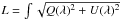 dλ/ Ic), net-circular polarization (NCP = |ΔV|/ ∫|V(λ)| dλ)3, and net-linear polarization (NLP = (|ΔQ| + |ΔU|)/ ∫|Q(λ)| +
|U(λ)| dλ)3. The distributions employed to characterize the statistical properties of the full FOV and subfields use 30 bins to sample the full domain of each quantity. Bins with fewer than 16 counts in the case of the subfields, or 25 in the case of the full FOV, are discarded. In the subfield selection procedure, all possible 29.52″ × 31.70″ subfields in the 302″ × 162″ FOV are considered. The selected subfield is the one that minimizes the sum of differences between the subfield distributions and the ones defined over the 302″ × 162″ domain. Figure 1 compares both the 302″ × 162″ region statistics and the selected subfield statistics, while Fig. 2 presents the selected subfield continuum intensity, the center-of-gravity magnetogram (COG; see Rees & Semel 1979), and the C, L, NCP, and NLP maps.
dλ/ Ic), net-circular polarization (NCP = |ΔV|/ ∫|V(λ)| dλ)3, and net-linear polarization (NLP = (|ΔQ| + |ΔU|)/ ∫|Q(λ)| +
|U(λ)| dλ)3. The distributions employed to characterize the statistical properties of the full FOV and subfields use 30 bins to sample the full domain of each quantity. Bins with fewer than 16 counts in the case of the subfields, or 25 in the case of the full FOV, are discarded. In the subfield selection procedure, all possible 29.52″ × 31.70″ subfields in the 302″ × 162″ FOV are considered. The selected subfield is the one that minimizes the sum of differences between the subfield distributions and the ones defined over the 302″ × 162″ domain. Figure 1 compares both the 302″ × 162″ region statistics and the selected subfield statistics, while Fig. 2 presents the selected subfield continuum intensity, the center-of-gravity magnetogram (COG; see Rees & Semel 1979), and the C, L, NCP, and NLP maps.
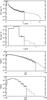 |
Fig. 1 Comparison between the statistical properties of the full 302″ × 162″ FOV (dashed line) and the statistical properties of the selected 29.52″ × 31.70″ subfield (solid line). From top to bottom: histogram of total circular polarization (C, first plot), total linear polarization (L, second plot), net-circular polarization (NCP, third plot), and net-linear polarization (NLP, fourth plot). The error bars are defined as the square root of the number of counts in each bin. |
3. Inversion hypothesis and strategy
We assign physical properties to each point of the portion of photosphere under examination by identifying a model atmosphere that reproduces Stokes profiles as close as possible to the observed ones. In the technical literature, this procedure is usually referred to as Stokes profile inversion. We perform the inversion based on the MISMA hypothesis. In a MIcro-Structured Magnetized Atmosphere, magnetic fields vary on scales smaller than the photon mean-free-path of the solar photosphere (Sánchez Almeida et al. 1996; Sánchez Almeida 1997). Starting from this hypothesis, Sánchez Almeida & Lites (2000) derived by inversion eleven classes of MISMA models representative of typical profiles observed in IN and network regions at the disk center.
All these models are formed by three components: one of them is field-free, while the other two are magnetized. The field-free component represents the non-magnetized plasma in which the magnetic fields are embedded, while the two magnetized components allow us to model the coexistence, in the resolution element, of different magnetic fields contributing to the formation of the observed polarization profiles. It has been shown by Sánchez Almeida et al. (1996, Sect. 4.2) that, based on the MISMA hypothesis, three is the minimum number of components with constant magnetic field required to reproduce the asymmetries of the Stokes profiles observed in the network, and three seem to suffice to reproduce all quiet Sun profiles (Sánchez Almeida & Lites 2000). These components should be considered as a schematic representation of the average properties of the atmosphere (see Sánchez Almeida & Lites 2000, Sect. 5). Each component of the model is characterized by the variation with height in the thermodynamical properties, plasma motions along the magnetic field lines, occupation fraction, and magnetic field strengths. These variations are forced to conserve magnetic flux and mass flows. The temperature stratification is imposed to be the same in the three optically thin components, since we expect an efficient radiative thermal exchange among them. Moreover, the lateral pressure balance links the properties of the components at every height; they must have the same total pressure defined as the sum of the gas pressure and the magnetic pressure. The mechanical balance couples the magnetic field with the thermodynamics in the model atmosphere. Magnetic field inclination and azimuth are constant with height. Finally, an unpolarized straylight contribution is considered (for a complete description of the inversion code and hypotheses, see Sánchez Almeida 1997; Sánchez Almeida & Lites 2000). The inversion of some 400 wavelengths defining each set of Stokes profiles employs only 20 free parameters, which is still twice the number of free parameters of ME inversions (Orozco Suárez et al. 2007c).
The adopted inversion strategy is the following. Stokes I and V are inverted in those pixels containing a |V| amplitude above 4.5 × σV at least for one wavelength in one of the two Fe i lines. If either the |Q| or |U| amplitude is above 4.5 × σQ,U, at least for one wavelength in one of the two Fe i lines, a full Stokes inversion is also performed. According to these criteria, about 29% of the subfield was inverted, with 2.3% corresponding to full Stokes inversions. The 4.5 × σQ,U,V thresholds were chosen to be the same as that of the ME inversion analyses already performed on our dataset (Orozco Suárez et al. 2007a; Asensio Ramos 2009). Each profile was inverted using as an initial guess all the eleven classes of MISMA models of Sánchez Almeida & Lites (2000). Among the eleven inversions, we select the one with the smallest deviation between the observed and the computed profiles. When only Stokes I and V are inverted, we assume the magnetic field to be longitudinal for both the magnetic components (i.e., the inclination is either zero or 180°). As we argue in Appendix A, this assumption influences the fraction of straylight inferred from the inversion, but not the magnetic field strength.
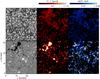 |
Fig. 2 Main observational properties of the representative 29.52″ × 31.70″ subfield selected for in-depth analysis. Continuum intensity (upper-left panel), total linear polarization (L, upper-central panel), net-linear polarization (NLP, upper-right panel), COG magnetogram saturated at ± 200 G (lower-left panel), total circular polarization (C, lower-central panel), and net-circular polarization (NCP, lower-right panel). The total polarization maps are both saturated at 1 pm, while the net-circular and net-linear polarization maps are saturated at 0.3. Black pixels in L, C, NLP, and NCP maps represent regions with signals below the threshold for inversion. The bars on top represent the color palettes adopted for the two pairs of images below them. |
3.1. Inversion examples
We now present examples of inversions. They were selected from all the 11 600 inverted profiles, and they are representative of the goodness of the fit.
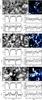 |
Fig. 3 Examples of MISMA inversion of HINODE SOT/SP Stokes profiles corresponding to mixed polarities in the resolution element. We show profiles in three different pixels representative of a weakly polarized IN region (upper panels), frontier pixels between regions with opposite polarity in the IN (central panels) and network (lower panels). The results are organized in two sets of panels; each of these sets contains an upper row with images that place the pixel in context, and a lower row with the four Stokes profiles (as labeled). The upper row shows l × l (l ≃ 6′′) maps of the COG magnetogram saturated at ±50 G (left), the continuum intensity (central), and the net-circular polarization saturated at 0.3 (right). The red square indicates the position from which the profiles are taken. Lower rows: observed Stokes profiles (symbols) and best-fit Stokes profiles (solid lines). The vertical dotted lines indicate the laboratory wavelengths of the two lines. |
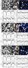 |
Fig. 4 Examples of MISMA inversion of HINODE SOT/SP Stokes profiles corresponding to a single polarity in the resolution element. For details of the layout of the figure, see the caption of Fig. 3. |
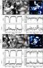 |
Fig. 5 Examples of full Stokes MISMA inversion of HINODE SOT/SP Stokes profiles. For details of the layout of the figure, see the caption of Fig. 3. |
Figure 3 shows three examples of pixels where the inversion code retrieves two opposite polarity fields coexisting in the resolution element. They were selected in different regions of the subfield, i.e., around the negative network patch at the top-left corner of Fig. 2, and in IN regions. The profiles show how the two polarities can be either easily detectable, when quasi-symmetric Stokes V profiles are measured, or almost hidden, when one of the two lobes of Stokes V almost vanishes. Two of the three selected cases coincide with a spatially-resolved large-scale change of polarity, i.e., the inverted pixels correspond to frontiers between positive and negative polarities in the COG magnetogram. In addition, the third example in Fig. 3 shows that mixed polarities can be found associated with polarized pixels that are not in frontiers between opposite polarities. We note that the three cases reported in Fig. 3 show no evidence of linear polarization signals above the 4.5 × σQ,U threshold. Even below the imposed threshold, the linear polarization profiles do not present any shape that could be interpreted by an inversion procedure with reliability.
Figure 4 contains three examples of profiles observed far from network regions. They were chosen to be characteristic of the typical profiles found in the IN as observed by HINODE SOT/SP. All Stokes V profiles display asymmetries, for which the inversion works in a really satisfactory way. The central panels of Figs. 3 and 4 correspond to adjacent pixels next to an apparent neutral line in COG magnetogram (i.e., where the magnetic field changes sign; we indicate their position on the magnetogram). They were selected to show how the MISMA inversion discerns between a single polarity model (Fig. 4) and a mixed polarity model (Fig. 3). The Stokes V profile in the central panel of Fig. 3 displays a dominant negative blue lobe, which is indicative the presence of negative fields. Apart from this, a small negative red lobe is also detected by the inversion. The latter denotes the presence of positive fields. The MISMA code correctly interprets this profile as emerging from a pixel in which opposite polarities coexist. This interpretation is consistent with the COG map, showing how the pixel from which the profile is taken lies in the frontier between positive and negative field patches. The central panel of Fig. 4 shows the Stokes V profile of a pixel next to the previous one in the direction of the positive polarity concentration. It is very different from its neighbor – the profile in Fig. 4 is dominated by a negative red lobe and presents a small positive blue lobe. The MISMA code interprets such a profile as emerging from a pixel in which only positive fields are present. In this case, the inversion is also consistent with the COG magnetogram, which shows the pixel lying on a positive polarity patch.
Figure 5 presents two examples of full Stokes inversion, i.e., inversions including Q and U. These examples illustrate the linear polarization signals we considered to be invertible. The upper panel of Fig. 5 shows the inversion of a pixel very close to the example in the lower panel of Fig. 3. In this case, the linear polarization signal is strong enough to be analyzed and the MISMA code succeeds in the inversion. We note that in such a pixel, as found in the lower panel of Fig. 3, polarization profiles are still interpreted by the code as emerging from a mixed polarity pixel. In the lower panel of Fig. 5, a full inversion of an IN pixel is represented. In this case, even if the pixel is almost on the boundary between opposite polarity regions, a single polarity is measured. In the two cases, the magnetic field strengths at the base of the photosphere are in the kG regime.
The examples discussed here illustrate not only the goodness of the fits but also the soundness of the MISMA interpretation of HINODE SOT/SP measurements. These measurements are often characterized by important asymmetries in Stokes V profiles; Figs. 3 and 4 show three examples of Stokes V profiles whose NCP ≥ 0.3. From the maps in Fig. 2, we note that these values for the NCP are very common in the selected 29.52″ × 31.70″ subfield and, by extrapolation, they should be very common in the full FOV as well. The common presence of large asymmetries demands a refined inversion method to interpret quiet Sun SOT/SP profiles, such as the MISMA inversion we employ. Detail of the percentage of asymmetric profiles are reported in Sect. 4.
4. Results
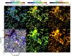 |
Fig. 6 Results of the inversion at the constant reference height, corresponding to the base of the photosphere. The different panels contain: classes of initial model MISMAs used in the inversion (upper-left panel), field strength for the minor component (upper-central panel), and occupation fraction for the minor component (upper-right panel), COG magnetogram saturated at ± 50 G (lower-left panel), field strength for the major component (lower-central panel), occupation fraction of the major component (lower-right panel). The contours in the COG magnetogram represent the network regions identified by our automatic procedure (red), and the pixels with mixed polarities in the resolution element (blue). Black pixels in the MISMA class, field strength, and occupation fraction maps correspond to regions that are not inverted (see Fig. 2). The bars at the top represent the color palettes adopted for the MISMA initial models (on the left), and for the two pairs of images of field strength (at the center) and occupation fraction (on the right). |
The inversion code succeeded in inverting 11 600 profiles, which represent 29% of the selected subfield. The total time needed to perform this analysis is about two days when the inversion analysis is divided into eight IDL jobs running in parallel4. Among the 11 600 inverted profiles, 925 (≃8% of the total number) show invertible linear polarization signals. These profiles were found mainly in correspondence with patches of strong polarization (see the upper panel in Fig. 5). Here we present the results obtained from the inversion of Stokes I and V profiles alone. Full Stokes inversions using modified MISMA models for which inclination and azimuth are free parameters were performed with success (e.g., Fig. 5), but their results are less representative than the ones from Stokes I and V inversions from a statistical point of view, and they provide similar results. Magnetic field strengths from few hG to kG fields are measured in fully inverted pixels, with a slightly higher probability for kG fields. We focus our analysis on the statistical properties of the magnetic field strength and occupation fraction at the photosphere as retrieved by the inversion code (the occupation fraction is just the volume filling factor). Assuming the model atmospheres to be in lateral pressure balance, each value of total pressure defines the same geometrical height in all model MISMAs. We decided to take as a reference height in the atmosphere the one corresponding to the base of the photosphere in typical 1D quiet Sun model atmospheres (e.g., Maltby et al. 1986). The photospheric lower boundary in these models is defined as the height where the continuum optical depth at 500 nm equals one, which corresponds to a pressure of about 1.3 × 10⁵ dyn cm-2. Unless otherwise mentioned explicitly, all the parameters discussed hereafter refer to this reference height or, equivalently, to this reference total pressure.
Figure 6 shows six maps summarizing the inversion at the reference height, and the COG magnetogram to illustrate the context. The red contours on the COG magnetogram distinguish network and IN regions in the selected subfield. Network patches were identified using an algorithm that takes into account two properties of the IN and network regions. First, the IN covers most of the solar photosphere at any time (more than 90% for Harvey-Angle 1993, which is the figure we use in the calculations). Second, network patches are magnetic concentrations showing a spatial coherence. The network must be identified not just as a strongly polarized region; it is expected to also be spatially extended. The procedure for defining the network works as follows: (1) It automatically finds the threshold of the total polarization that makes the patches of large signal covering a few percent of the FOV (≃4%). These signals are tentatively identified as cores of network elements; (2) It verifies the spatial extension of the network patch candidates so as to exclude connected structures consisting of fewer than ten pixels. Once the network patches have been identified, the procedure dilates them using a 10 × 10 pixel square kernel. The network patches thus selected cover 11% of the subfield.
At the location of the network patches, the map showing the initial guess models for the inversion of each pixel reveals a significant degree of local coherence (Fig. 6, top left panel). In contrast, the initial model MISMA fluctuates in the IN on scales smaller than 1″. Considering the network and IN together, the percentages of different types of best initial guess models are class 0 ≃ 5%, class 1 ≃ 18%, class 2 ≃ 16%, class 3 ≃ 10%, class 4 ≃ 11%, class 5 ≃ 0%, class 6 ≃ 7%, class 7 ≃ 12%, class 8 ≃ 14%, class 9 ≃ 5%, and class 10 ≃ 0% (see Sánchez Almeida & Lites 2000, for a detailed description of the classes). The initial model MISMAs can be used as a proxy of the asymmetries present in HINODE spectra. We find that 35% of the inverted profiles belong to classes 4, 6, 7, and 9. These are the classes where Stokes V exhibits large asymmetries, similar to those shown in Figs. 3 and 4.
The central panels of Fig. 6 display the magnetic field strengths of the two magnetized components of the model MISMAs. The results are organized so that the major and the minor components are considered separately5. On the one hand, the major component has occupation fractions (equivalent to volume-filling factors) from ~10-2 to ≳10-1, and magnetic field strengths between 0 G and 1.8 kG. On the other hand, the minor component has a filling factor of almost always ≲10-2 and field strengths ≳1 kG. Only in the network patches does the minor component display filling factor values comparable to those of the major component.
The statistical properties of the field strength for both the major and minor components are reported in Fig. 7. The figure indicates the fraction of analyzed photosphere covered by a given field strength PZ(B), i.e., except for a scaling factor, it gives the sum of all occupation fractions for each magnetic field strength B. The histograms were defined by sampling the interval 0−2 kG with 20 bins of 100 G. They show the probability of finding a given field strength in our quiet Sun inversion. The distribution corresponding to the whole subfield presents a maximum at ≃1.6 kG, and then an extended tail for lower field strengths. The statistics for the IN regions (Fig. 7, top, thick solid line) infer that they contain kG fields, with a secondary maximum at the equipartition value of ≃5 hG. We note the reduction in the kG peak with respect to the full subfield distribution (Fig. 7, top, thin solid line). It is clear that the hG fields are almost completely in the IN, while the network is dominated by kG fields with little contribution for fields in the hG regime. On the other hand, the statistics of the minor component is completely dominated by strong kG fields with a maximum at 1.8 kG alone and an almost null hG contribution; this is valid for the whole subfield, IN, and network.
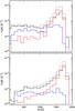 |
Fig. 7 Fraction of analyzed photosphere covered by a given strength. Field strength distributions for the major component (upper panel): IN (black thick line), network (red line), mixed polarity regions (blue line), and the full 29.52″ × 31.70″ subfield (black thin line). Field strength distributions for the minor component (lower panel). |
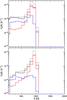 |
Fig. 8 Fraction of analyzed photosphere covered by a given strength at 150 km height in MISMA models. For details of the layout of the figure, see the caption of Fig. 7. |
The magnetic field strength distribution in Fig. 8 is calculated for a height in the atmosphere of approximatively 150 km, i.e., a height representative of the formation region of the core of the Fe i lines. As when defining the reference height of the photosphere, the heights are selected to be those of a total pressure of 4 × 10⁴ dyn cm-2 (at approximatively 150 km in the pressure stratification of the mean photosphere; e.g. Maltby et al. 1986). The main difference between the two statistics in Figs. 7 and 8 is the large reduction in kG fields at 150 km. The magnetic structures are treated as thin fluxtubes by the inversion code, hence the magnetic field lines must fan out with height to maintain the mechanical equilibrium, leading to a drop in field strength and an expansion of the magnetic structures (e.g., Spruit 1981). These two factors conspire to produce the observed increase in hG fields with height (cf. Figs. 7 and 8). For example, the volume occupied by magnetic fields weaker than 1 kG at 150 km is some 8 times stronger than their volume at the base of the photosphere.
A very interesting result, unique to MISMA inversions, is the detection of a large number of mixed polarity pixels (three examples are reported in Fig. 3). These are identified by the blue contours in the COG magnetogram of Fig. 6. Pixels with mixed polarities are very common to IN, namely about 25% of the total number of inverted profiles. In contrast, network patches tend to be interpreted by the code as unipolar regions. We note that mixed polarities show up almost always either in the boundaries between strong signals of opposite polarity, or in low polarization regions, close to the 4.5 × σV level. We also note the presence of mixed polarities surrounding the large negative polarity network patch in the selected subfield (see the upper left corner in the COG magnetogram in Fig. 6). They are always found where positive small concentrations are close to the network patch. Figure 7 also includes the statistical properties of the mixed polarity pixels separately. In contrast to the other statistics described above, the distribution for mixed polarity pixels is not dominated by kG fields: hG and kG fields are found almost with the same occupation fraction in both IN and network regions, and for both minor and major components. The distribution has an absolute maximum at about 1.6 kG and a secondary one at about 500 G.
The fraction of analyzed photosphere occupied by magnetic fields α can be computed as the integral of the distributions in Fig. 7, i.e., 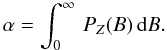 (1)The value of α for the major and the minor components across the full subfield is 3.1% and 1.4%, respectively. In other words, 95.5% of the analyzed photosphere is field free or, more precisely, it has field strengths much weaker than those inferred from inversion, so the inversion code cannot distinguish them from zero. Other fractions corresponding to the various components in the FOV are listed in Table 1. The first moment of the magnetic field strength distributions also provides an estimate of the unsigned flux density ⟨ B ⟩ (see, e.g., Domínguez Cerdeña et al. 2006b)
 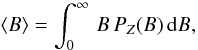 (2)and of the average field strength
  (3)The values of ⟨ B ⟩ and
  for the various components in the FOV are listed in Table 1. As the table shows, ⟨ B ⟩ = 66 G for both the network and IN together. This flux density is so high partly because it reflects the fraction of the 29.52″ × 31.70″ subfield with the largest polarization signals. This fraction f is about 0.29, therefore, if one considers the full subfield, the fraction of photosphere occupied by the magnetic fields inferred from our inversion is αf, and the unsigned flux density is ⟨ B ⟩ f. The values of the filling factor and unsigned flux densities corresponding to this other normalization are also included in Table 1 within parentheses. The unsigned flux density then decreases to about 19 G. This still large value is placed in context in Sect. 5, but it is important to realize that it implicitly assumes the (1 − f) non-inverted subfield to have no magnetic fields.
We also tried a crude separation between granules and intergranules. A simple thresholding criterion was used, so that pixels brighter than the mean intensity are granules, and vice-versa. We find that 75% of the magnetized plasma is in intergranules, and this fraction increases with increasing field strength – 85% of the plasma with B > 1.5 kG is contained in intergranules. These figures are meant to be rough estimates since our simple criterion is insufficient for an accurate separation between granules and intergranules.
5. Discussion
Summary of magnetic properties at the base of the photosphere derived from the MISMA inversion.
The ubiquity of Stokes profiles with asymmetries implies that even the HINODE SOT/SP resolution is insufficient to resolve the structure of the quiet Sun magnetic fields (see Sánchez Almeida et al. 1996). This unresolved structure has been neglected in the analyses carried out so far, and we have presented the first attempt to account for it when interpreting HINODE spectra. We have employed the MISMA inversion code by Sánchez Almeida (1997), which produces very good fits. The MISMA description is able to reproduce the whole range of profile shapes observed by HINODE SOT/SP in the quiet Sun, which are often extremely asymmetric. This was known to be true for Advanced Stokes Polarimeter (ASP) spectra (Sánchez Almeida & Lites 2000), but the HINODE SOT/SP has three times the spatial resolution of ASP (i.e., 0.3″ against 1″).
The percentages of MISMA classes used as initial guesses differ from those reported in Sánchez Almeida & Lites (2000). This may be due to either the inversion strategy (e.g., the imposed threshold to select invertible data) or a general modification of Stokes profile shapes caused by the higher spatial resolution.
As pointed out in Sánchez Almeida & Lites (2000), the major component is the dominant source of polarization of the model since it contains the highest mass. For this reason, the statistics of the major component is assumed to be the reference statistics derived from our analysis. The field strength distribution of the major component differs significantly from the results of Sánchez Almeida & Lites (2000); our analysis is able to reveal far more hG fields than the analysis of the ASP data. These are almost completely within the IN, and a large part of them are found in mixed polarity pixels. Moreover, the statistics of the latter indicates that hG and kG fields are measured with the same probability. The IN kG magnetic fields are more important in our inversion than the inversions carried out by Orozco Suárez et al. (2007a) and Asensio Ramos (2009). Part of this difference is certainly due to their use of ME atmospheres, which are unable to reproduce the important line asymmetries characteristic of the quiet Sun Stokes profiles. This difficulty may be secondary when dealing with slightly asymmetrical profiles, but the field strengths are inferred from the Stokes V shapes, and any field strength extracted by fitting anti-symmetric ME profiles to profiles such as those in Figs. 3 and 4 is open to question. Another part of the difference can come from the large drop in magnetic field strength with height in the atmosphere. As discussed in Domínguez Cerdeña et al. (2006b) and in Sect. 4, a reduction in the magnetic pressure is required to maintain the mechanical balance between the magnetic structures and the field-free atmosphere when the gas pressure decreases exponentially with height. This decrease in field strength is intrinsic to the MISMA models, which force their components to be in horizontal and vertical mechanical equilibrium. Orozco Suárez et al. (2007b) showed that the ME inversion of Fe i 630 nm gives us information on the solar atmosphere at the height of formation of the lines, which is higher than the reference height adopted in this work. When the magnetic field strength statistics are calculated at a height of 150 km, then kG fields are almost absent (Fig. 8), which partly reconciles our results with those inferred from ME inversions. However, the shape of our distribution still differs from the one reported in Orozco Suárez et al. (2007a) in which the most probable field strength is ≃100 G.
Three additional comments about the field strength distribution are in order. First, kG fields are needed to explain the presence of G-band bright points in the quiet Sun intergranular lanes (e.g., Sánchez Almeida et al. 2004; de Wijn et al. 2005; Bovelet & Wiehr 2008; Sánchez Almeida et al. 2010) and, therefore, it is a sign of consistency that they show up in spectropolarimetric observations. The occupation fraction of kG fields inferred from the inversion is of the order of a few percent, which is in good agreement with the 0.5−2% G-band bright point surface coverage that has been measured (Sánchez Almeida et al. 2004; Bovelet & Wiehr 2008; Sánchez Almeida et al. 2010). Moreover, the strong polarization signals that we select for inversion appear preferentially in the intergranular lanes (Domínguez Cerdeña et al. 2003a; Lites et al. 2008) where the BPs are known to reside. Second, our results do not exclude the presence of weak fields (i.e., fields producing weak polarization signals in the Fe i visible lines). Our inversion retrieves the field strength of only 4.5% of the photospheric plasma (see Sect. 4). The field strength of the rest remains unconstrained. This part is almost certainly magnetic, but with properties that remain elusive to our observation because of its complex magnetic topology that cancels the Zeeman signals, because of the low field strengths, or both. Sánchez Almeida et al. (2003) and Domínguez Cerdeña et al. (2006a) show how part of these hidden fields can be revealed by means of MISMA inversion by analyzing Fe i infra-red lines. Even weaker fields can be inferred and diagnosed by applying Hanle effect (e.g., Faurobert-Scholl 1994; Bommier et al. 2005). To avoid overlooking the weak field component, the quiet Sun regions need to be analyzed using measurements for both the visible and infra-red spectral ranges, and produced by both the Zeeman and Hanle effects. How to consistently combine these measurements remains an open issue, but this combination is certainly the way to go (see the first attempt by Domínguez Cerdeña et al. 2006b). The third comment on the field strength distribution refers to discarding biases that may artificially produce kG fields. Bellot Rubio & Collados (2003) show how substantial noise in the Stokes V profiles of the Fe i 630 nm lines can mimic kG fields. However, this effect is insignificant above a signal-to-noise ratio threshold that our typical spectra exceed. Moreover, in addition to kG, noise also produces false weak dG, which we do not see. Another potential source of false kG fields could be (polarized) straylight from the network to the IN. Although we cannot discard some influence close to the network patches, straylight cannot account for the bulk of the kG fields in the IN. Straylight is at most 10% as measured for the broadband filter imager aboard HINODE (Wedemeyer-Böhm 2008). It may account for 10% of the network magnetic flux artificially appearing in the IN, but this represents only a few G, thus is unable to explain the some 30 G inferred for the IN (see Table 1).
The mixed polarity regions revealed by the MISMA analysis are about 25% of the total number of inverted profiles, similar to the percentage reported in Sánchez Almeida & Lites (2000) for ASP data (see also Socas-Navarro & Sánchez Almeida 2002). We note that the percentage of mixed polarities has not changed despite the increase in angular resolution (from 1″ to 0.3″) and the polarization signals analyzed here being generally stronger (we use a noise threshold 1.5 times larger than the one used on ASP spectra). The really significant difference between the two datasets is the fraction of solar surface covered by polarization signals; Sánchez Almeida & Lites (2000) invert only 15% of the surface, whereas HINODE spectra allow us to almost double this fraction. The increase in angular resolution has certainly resolved some of the mixed polarities detected at ASP angular resolution, although, at the same time, the newly revealed Stokes V profiles uncover mixed polarities on even finer spatial scales. This observation is consistent with the numerical models of solar magneto-convection and/or turbulent dynamos (e.g., Cattaneo 1999; Vögler & Schüssler 2007). They predict an intricate pattern of highly intermittent fields varying over very small spatial scales down to the diffusion length-scales.
The average flux density we infer from the inverted profiles is of the order of 19 G when the area of the full subfield is considered for normalization (see Table 1). This value is almost twice as high as the one inferred by Sánchez Almeida & Lites (2000, 1″, and it is also significantly higher than the ones obtained from ME inversions of quiet Sun HINODE spectra by Orozco Suárez et al. (2007a, ~9.5, and using the magnetograph equation by Lites et al. (2008, 11. However, our estimate is comparable with other HINODE-based estimates of the unsigned flux of the quiet Sun (e.g., Jin et al. 2009 get 28 G). This difference could be explained by taking into account that ME inversions are blind to sub-pixel magnetic structuring. We note that the average flux density from the major component (i.e., the dominant source of polarization) is in good agreement with that measured by Orozco Suárez et al. (2007a) and Lites et al. (2008) – we derive 12.5 G (see Table 1). The small excess with respect to their results is compatible with the 1.6 G flux contribution from mixed polarities (see Table 1). The bulk of the difference seems to reside in the 6.7 G provided by the minor component. Its contribution to the flux density is more important than the modification it produces to the polarization signals (even though it is needed to reproduce the line asymmetries).
6. Conclusions
We have presented the first inversion of HINODE SOT/SP Stokes profiles that accounts for the asymmetries of the profiles in the quiet Sun. The analysis has been carried out based on the MISMA hypotheses, which allows us to reproduce the different profile shapes observed in the quiet Sun. We have followed an approach already successfully exploited to describe the asymmetries observed with 1″ angular resolution (Sánchez Almeida & Lites 2000).
The main results are as follows:
-
1.
We have inverted sets of Stokes I and V profiles representative of the quiet Sun internetwork (IN) and network at disk center. The inversion code is able to reproduce, in a satisfactory way, the whole variety of asymmetries revealed by HINODE SOT/SP.
-
2.
The MISMA code is also able to reproduce linear polarization measurements when full Stokes inversions are performed. Here we report a few examples.
-
3.
The existence of asymmetries is certainly not negligible. Some 35% of the analyzed profiles display large asymmetries, according to the rough classification used in Sánchez Almeida & Lites (2000).
-
4.
About 25% of the analyzed profiles display asymmetries that are interpreted by the MISMA code as due to mixed polarities in the resolution element. These pixels are found to be located in either transition regions between patches of opposite polarity, or pixels containing weak polarization signals.
-
5.
The magnetic plasma whose properties the inversion code constrains represents only 4.5% of the photospheric plasma. The remainder remains unconstrained by our analysis.
-
6.
The statistics of the detected magnetic field strength at the formation height of the continuum are dominated by strong kG fields, in both the network and the IN. The IN, however, exhibits an extended tail over the whole hG domain.
-
7.
At the height of 150 km (representative of the formation heights of the Fe i visible lines), only extremely faint kG fields are measured. This result narrows down the gap between our field strength distribution and those inferred from ME inversions by Orozco Suárez et al. (2007a) and Asensio Ramos (2009), and follows directly from the decrease in the field strength in response to the decrease in the gas pressure with height in the photosphere.
-
8.
The average flux density derived from the inverted pixels is 66 G. If one considers the full analyzed subfield, it becomes 19 G. The same figures for the IN become 32 G and 9.3 G, respectively. These values are significantly larger than the ones obtained from ME inversions of quiet Sun HINODE spectra by Orozco Suárez et al. (2007a, ~, and using the magnetograph equation by Lites et al. (2008, 11. However, our estimate is comparable to other HINODE-based estimates of the unsigned flux of the quiet Sun (e.g., Jin et al. 2009 get 28 G).
As a general concluding remark, the analysis presented here reveals the importance of a complete interpretation of the shape of Stokes V profiles by means of refined inversion codes. This work should be considered as the first step in the interpretation of HINODE SOT/SP profile shapes. Because of the wealth of information contained in the asymmetries, this topic deserves the attention of the solar community. Different inversion codes and hypotheses can be adopted to interpret these asymmetries, and they will probably also be able to reproduce the line shapes (e.g., a systematic variation in magnetic field and velocity along the LOS; Ruiz Cobo & del Toro Iniesta 1992). The uniqueness of the interpretation cannot be assessed unless different alternatives agree.
ME codes consider the existence of a field-free atmosphere portion in the resolution element via a straylight filling factor (see e.g., Skumanich & Lites 1987; Orozco Suárez et al. 2007a).
Each wavelength window is defined by two wavelengths (λA and λB) centered around the wavelength of the Stokes I minimum (λm). The width of the window centered on the Fe i 630.15 nm line is 86 pm, while for Fe i 630.25 nm the width is 64 pm.
 d
d dλ, where S can be Q,U, or V, and λA, λB, and λm are defined in footnote2.
The inversion of each pixel is independent, so the analysis of the invertible domain can be distributed over different CPUs; the jobs are run on two Xeon E5410 Quad-core processors with 8 GB of shared ram.
In each pixel, the major and the minor components are the magnetized components of the highest and lowest mass, respectively.
Acknowledgments
HINODE is a Japanese mission developed and launched by ISAS/JAXA, with NAOJ as domestic partner and NASA and STFC (UK) as international partners. It is operated by these agencies in co-operation with ESA and NSC (Norway). J.S.A. acknowledges the support provided by the Spanish Ministry of Science and Technology through project AYA2007-66502, as well as by the EC SOLAIRE Network (MTRN-CT-2006-035484). This work was partially supported by ASI grant n.I/015/07/0ESS.
References
- Asensio Ramos, A. 2009, ApJ, 701, 1032 [NASA ADS] [CrossRef] [Google Scholar]
- Bellot Rubio, L. R., & Collados, M. 2003, A&A, 406, 357 [NASA ADS] [CrossRef] [EDP Sciences] [Google Scholar]
- Bommier, V. Derouich, M. Landi Degl’ Innocenti, E., Molodij, G., & Sahal-Bréchot, S. 2005, A&A, 432, 295 [NASA ADS] [CrossRef] [EDP Sciences] [Google Scholar]
- Bovelet, B., & Wiehr, E. 2008, A&A, 488, 1101 [NASA ADS] [CrossRef] [EDP Sciences] [Google Scholar]
- Cattaneo, F. 1999, ApJ, 515, L39 [NASA ADS] [CrossRef] [Google Scholar]
- Centeno, R., Socas-Navarro, H., Lites, B., et al. 2007, ApJ, 666, L137 [NASA ADS] [CrossRef] [Google Scholar]
- de Wijn, A. G., Rutten, R. J., Haverkamp, E. M. W. P., & Sütterlin, P. 2005, A&A, 441, 1183 [NASA ADS] [CrossRef] [EDP Sciences] [Google Scholar]
- Domínguez Cerdeña, I. Kneer, F. & Sánchez Almeida, J. 2003, ApJ, 582, L55 [NASA ADS] [CrossRef] [Google Scholar]
- Domínguez Cerdeña, I. Sánchez Almeida, J., & Kneer, F. 2006a, ApJ, 646, 1421 [NASA ADS] [CrossRef] [Google Scholar]
- Domínguez Cerdeña, I. Sánchez Almeida, J., & Kneer, F. 2006b, ApJ, 636, 496 [NASA ADS] [CrossRef] [Google Scholar]
- Faurobert-Scholl, M. 1994, A&A, 285, 655 [NASA ADS] [Google Scholar]
- Fischer, C. E., de Wijn, A. G., Centeno, R., Lites, B. W., & Keller, C. U. 2009, A&A, 504, 583 [NASA ADS] [CrossRef] [EDP Sciences] [Google Scholar]
- Harvey-Angle, K. L. 1993, Ph.D. Thesis, Utrecht University, The Netherlands [Google Scholar]
- Ichimoto, K., Lites, B., & Elmore, A. O. 2008, Sol. Phys., 249, 233 [NASA ADS] [CrossRef] [Google Scholar]
- Jin, C., Wang, J., & Zhao, M. 2009, ApJ, 690, 279 [NASA ADS] [CrossRef] [Google Scholar]
- Kosugi, T., Matsuzaki, K., Sakao, T., et al. 2007, Sol. Phys., 243, 3 [NASA ADS] [CrossRef] [Google Scholar]
- Landi Degl’Innocenti, E. 1994a, in Solar Surface Magnetism, ed. R. J. Rutten, & C. J. Schrijver, 29 [Google Scholar]
- Landi Degl’Innocenti, E. 1994b, in Solar Surface Magnetism, ed. R. J. Rutten, & C. J. Schrijver, 29 [Google Scholar]
- Lites, B. W., Elmore, D. F., & Streander, K. V. 2001, in Advanced Solar Polarimetry – Theory, Observation, and Instrumentation, ed. M. Sigwarth, ASP Conf. Ser., 236, 33 [Google Scholar]
- Lites, B. W., Kubo, M., Socas-Navarro, H., et al. 2008, ApJ, 672, 1237 [NASA ADS] [CrossRef] [Google Scholar]
- Maltby, P., Avrett, E. H., Carlsson, M., et al. 1986, ApJ, 306, 284 [Google Scholar]
- Nagata, S., Tsuneta, S., Suematsu, Y., et al. 2008, ApJ, 677, L145 [NASA ADS] [CrossRef] [Google Scholar]
- Orozco Suárez, D., Bellot Rubio, L. R., del Toro Iniesta,, et al. 2007a, ApJ, 670, L61 [NASA ADS] [CrossRef] [Google Scholar]
- Orozco Suárez, D., Bellot Rubio, L. R. & del Toro Iniesta, J. C. 2007b, ApJ, 662, L31 [NASA ADS] [CrossRef] [Google Scholar]
- Suárez, D., Bellot Rubio, L. R. Del Toro Iniesta, J. C., et al. 2007c, PASJ, 59, 837 [Google Scholar]
- Orozco Suárez, D., Bellot Rubio, L. R. del Toro Iniesta, J. C., & Tsuneta, S. 2008, A&A, 481, L33 [NASA ADS] [CrossRef] [EDP Sciences] [Google Scholar]
- Rees, D. E., & Semel, M. D. 1979, A&A, 74, 1 [NASA ADS] [Google Scholar]
- Ruiz Cobo, B. & del Toro Iniesta, J. C. 1992, ApJ, 398, 375 [NASA ADS] [CrossRef] [Google Scholar]
- Sánchez Almeida, J. 1997, ApJ, 491, 993 [NASA ADS] [CrossRef] [Google Scholar]
- Sánchez Almeida, J. 2004, in The Solar-B Mission and the Forefront of Solar Physics, ed. T. Sakurai, & T. Sekii, ASP Conf. Ser., 325, 115 [Google Scholar]
- Sánchez Almeida, J., & Ichimoto, K. 2009, A&A, 508, 963 [NASA ADS] [CrossRef] [EDP Sciences] [Google Scholar]
- Sánchez Almeida, J., & Lites, B. W. 2000, ApJ, 532, 1215 [NASA ADS] [CrossRef] [Google Scholar]
- Sánchez Almeida, J. & Trujillo Bueno, J. 1999, ApJ, 526, 1013 [NASA ADS] [CrossRef] [Google Scholar]
- Sánchez Almeida, J. Landi Degl’Innocenti, E. Martinez Pillet, V., & Lites, B. W. 1996, ApJ, 466, 537 [NASA ADS] [CrossRef] [Google Scholar]
- Sánchez Almeida, J. Domínguez Cerdeña, I., & Kneer, F. 2003, ApJ, 597, L177 [NASA ADS] [CrossRef] [Google Scholar]
- Sánchez Almeida, J. Márquez, I. Bonet, J. A. Domínguez Cerdeña, I., & Muller, R. 2004, ApJ, 609, L91 [NASA ADS] [CrossRef] [Google Scholar]
- Sánchez Almeida, J. Bonet, J. A. Viticchié, B. & Del Moro, D. 2010, ApJ, 715, L26 [NASA ADS] [CrossRef] [Google Scholar]
- Shimizu, T., Lites, B. W., Katsukawa, Y., et al. 2008, ApJ, 680, 1467 [NASA ADS] [CrossRef] [Google Scholar]
- Skumanich, A., & Lites, B. W. 1987, ApJ, 322, 473 [Google Scholar]
- Socas-Navarro, H. & Sánchez Almeida, J. 2002, ApJ, 565, 1323 [NASA ADS] [CrossRef] [Google Scholar]
- Spruit, H. C. 1981, A&A, 102, 129 [NASA ADS] [Google Scholar]
- Stenflo, J. O. 2009, Mem. Soc. Astron. Ital., 80, 690 [NASA ADS] [Google Scholar]
- Tsuneta, S., Ichimoto, K., Katsukawa, Y., et al. 2008, Sol. Phys., 249, 167 [NASA ADS] [CrossRef] [Google Scholar]
- Vögler, A., & Schüssler, M. 2007, A&A, 465, L43 [NASA ADS] [CrossRef] [EDP Sciences] [Google Scholar]
- Wedemeyer-Böhm, S. 2008, A&A, 487, 399 [NASA ADS] [CrossRef] [EDP Sciences] [Google Scholar]
- Zhang, J., Yang, S.-H., & Jin, C.-L. 2009, Res. Astron. Astrophys., 9, 921 [NASA ADS] [CrossRef] [Google Scholar]
Appendix A: Lack of crosstalk between magnetic field strength and magnetic field inclination
When Q and U are too small to be used, the inversions assume the magnetic field to be longitudinal. It is important to realize that this assumption does not influence our magnetic field strength diagnostics. When the polarizations signals are weak (our case), and the inclination is constant (our assumption), then Stokes V scales with the cosine of the inclination independently of the field strength (Sánchez Almeida & Trujillo Bueno 1999, Sect. 3.1). The information about the field strength is coded in the shape of Stokes V, whereas the magnetic field inclination modifies the scaling. This scaling is independently obtained by the inversion code disguised as straylight, therefore the inferred magnetic field strength and inclination are uncoupled. All quiet Sun inversions assume the pixels to be partly covered by magnetic fields, and the corresponding filling factor is determined as a free parameter of the inversion (straylight factor). An error in the magnetic field inclination affects the straylight factor, but it does not influence the magnetic field determination. Figure A.1 illustrates the argument. It shows Stokes I and V synthesized in two atmospheres that differ in straylight factor fsl and cosine of inclination cosθ, but they have the same product cosθ (1 − fsl). The two pairs of Stokes profiles are indistinguishable within the noise of HINODE observations.
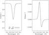 |
Fig. A.1 Two sets of synthetic Stokes I and V profiles of Fe i 630.25 nm obtained with different magnetic field inclinations θ but the same product (1 − fsl) cosθ, with fsl the fraction of straylight. The solid and the dotted lines correspond to θ = 0°and 60°, respectively. The two sets cannot be distinguished within typical HINODE noise. |
All Tables
Summary of magnetic properties at the base of the photosphere derived from the MISMA inversion.
All Figures
|
Fig. 1 Comparison between the statistical properties of the full 302″ × 162″ FOV (dashed line) and the statistical properties of the selected 29.52″ × 31.70″ subfield (solid line). From top to bottom: histogram of total circular polarization (C, first plot), total linear polarization (L, second plot), net-circular polarization (NCP, third plot), and net-linear polarization (NLP, fourth plot). The error bars are defined as the square root of the number of counts in each bin. |
| In the text | |
|
Fig. 2 Main observational properties of the representative 29.52″ × 31.70″ subfield selected for in-depth analysis. Continuum intensity (upper-left panel), total linear polarization (L, upper-central panel), net-linear polarization (NLP, upper-right panel), COG magnetogram saturated at ± 200 G (lower-left panel), total circular polarization (C, lower-central panel), and net-circular polarization (NCP, lower-right panel). The total polarization maps are both saturated at 1 pm, while the net-circular and net-linear polarization maps are saturated at 0.3. Black pixels in L, C, NLP, and NCP maps represent regions with signals below the threshold for inversion. The bars on top represent the color palettes adopted for the two pairs of images below them. |
| In the text | |
|
Fig. 3 Examples of MISMA inversion of HINODE SOT/SP Stokes profiles corresponding to mixed polarities in the resolution element. We show profiles in three different pixels representative of a weakly polarized IN region (upper panels), frontier pixels between regions with opposite polarity in the IN (central panels) and network (lower panels). The results are organized in two sets of panels; each of these sets contains an upper row with images that place the pixel in context, and a lower row with the four Stokes profiles (as labeled). The upper row shows l × l (l ≃ 6′′) maps of the COG magnetogram saturated at ±50 G (left), the continuum intensity (central), and the net-circular polarization saturated at 0.3 (right). The red square indicates the position from which the profiles are taken. Lower rows: observed Stokes profiles (symbols) and best-fit Stokes profiles (solid lines). The vertical dotted lines indicate the laboratory wavelengths of the two lines. |
| In the text | |
|
Fig. 4 Examples of MISMA inversion of HINODE SOT/SP Stokes profiles corresponding to a single polarity in the resolution element. For details of the layout of the figure, see the caption of Fig. 3. |
| In the text | |
|
Fig. 5 Examples of full Stokes MISMA inversion of HINODE SOT/SP Stokes profiles. For details of the layout of the figure, see the caption of Fig. 3. |
| In the text | |
|
Fig. 6 Results of the inversion at the constant reference height, corresponding to the base of the photosphere. The different panels contain: classes of initial model MISMAs used in the inversion (upper-left panel), field strength for the minor component (upper-central panel), and occupation fraction for the minor component (upper-right panel), COG magnetogram saturated at ± 50 G (lower-left panel), field strength for the major component (lower-central panel), occupation fraction of the major component (lower-right panel). The contours in the COG magnetogram represent the network regions identified by our automatic procedure (red), and the pixels with mixed polarities in the resolution element (blue). Black pixels in the MISMA class, field strength, and occupation fraction maps correspond to regions that are not inverted (see Fig. 2). The bars at the top represent the color palettes adopted for the MISMA initial models (on the left), and for the two pairs of images of field strength (at the center) and occupation fraction (on the right). |
| In the text | |
|
Fig. 7 Fraction of analyzed photosphere covered by a given strength. Field strength distributions for the major component (upper panel): IN (black thick line), network (red line), mixed polarity regions (blue line), and the full 29.52″ × 31.70″ subfield (black thin line). Field strength distributions for the minor component (lower panel). |
| In the text | |
|
Fig. 8 Fraction of analyzed photosphere covered by a given strength at 150 km height in MISMA models. For details of the layout of the figure, see the caption of Fig. 7. |
| In the text | |
|
Fig. A.1 Two sets of synthetic Stokes I and V profiles of Fe i 630.25 nm obtained with different magnetic field inclinations θ but the same product (1 − fsl) cosθ, with fsl the fraction of straylight. The solid and the dotted lines correspond to θ = 0°and 60°, respectively. The two sets cannot be distinguished within typical HINODE noise. |
| In the text | |
Current usage metrics show cumulative count of Article Views (full-text article views including HTML views, PDF and ePub downloads, according to the available data) and Abstracts Views on Vision4Press platform.
Data correspond to usage on the plateform after 2015. The current usage metrics is available 48-96 hours after online publication and is updated daily on week days.
Initial download of the metrics may take a while.