| Issue |
A&A
Volume 526, February 2011
|
|
|---|---|---|
| Article Number | A158 | |
| Number of page(s) | 30 | |
| Section | Numerical methods and codes | |
| DOI | https://doi.org/10.1051/0004-6361/201015340 | |
| Published online | 14 January 2011 | |
The impact of numerical viscosity in SPH simulations of galaxy clusters
SISSA/ISAS, via Bonomea 265,
34136
Trieste,
Italy
e-mail: valda@sissa.it
Received: 6 July 2010
Accepted: 14 October 2010
The goal of this paper is to investigate in N-body/SPH hydrodynamical cluster simulations the impact of artificial viscosity on the ICM thermal and velocity field statistical properties. To properly reduce the effects of artificial viscosity, a time-dependent artificial viscosity scheme is implemented in an SPH code in which each particle has its own viscosity parameter, whose time evolution is governed by the local shock conditions. The new SPH code is verified in a number of test problems with known analytical or numerical reference solutions and is then used to construct a large set of N-body/SPH hydrodynamical cluster simulations. These simulations are designed to study in SPH simulations the impact of artificial viscosity on the thermodynamics of the ICM and its velocity field statistical properties by comparing results extracted at the present epoch from runs with different artificial viscosity parameters, cluster dynamical states, numerical resolution, and physical modeling of the gas.
Spectral properties of the gas velocity field are investigated by measuring the velocity power spectrum E(k) for the simulated clusters. Over a limited range, the longitudinal component Ec(k) exhibits a Kolgomorov-like scaling ∝ k−5/3, whilst the solenoidal power spectrum component Es(k) is strongly influenced by numerical resolution effects. The dependence of the spectra E(k) on dissipative effects is found to be significant at length scales ≲100−300 kpc, with viscous damping of the velocities being less pronounced in the runs with the lowest artificial viscosity. The turbulent energy density radial profile Eturb(r) is strongly affected by the numerical viscosity scheme adopted in the simulations, with the turbulent-to-total energy density ratios being higher in the runs with the lowest artificial viscosity settings and lying in the range between a few percent and ~10%. These values are in accord with the corresponding ratios extracted from previous cluster simulations based on mesh-based codes.
The radial entropy profiles show a weak dependence on the artificial viscosity parameters of the simulations, with a small amount of entropy mixing being present in cluster cores. At large cluster radii, the mass correction terms to the hydrostatic equilibrium equation are affected little by the numerical viscosity of the simulations, indicating that the X-ray mass bias is already accurately estimated in standard SPH simulations.
The results presented here indicate that in individual SPH cluster simulations at least N ≳ 2563 gas particles are necessary to provide a correct description of turbulent spectral properties over a decade in wavenumbers, whilst radial profiles of thermodynamic variables can be reliably obtained using N ≳ 643 particles. Finally, simulations in which the gas can cool radiatively are characterized by the presence in the cluster inner regions of high levels of turbulence, generated by the interaction of the compact cool gas core with the ambient medium. These findings strongly support the viability of a turbulent heating model in which radiative losses in the core are compensated by heat diffusion and viscous dissipation of turbulent motion.
Key words: galaxies: clusters: general / X-rays: galaxies: clusters / methods: numerical
© ESO, 2011
1. Introduction
According to the standard hierarchical scenario, the formation of larger structures is driven by gravity and proceeds hierarchically through merging and accretion of smaller size halos. Within this scenario, galaxy clusters are the most recent and the largest virialized objects known in the universe. Their formation and evolution rate is then a strong function of the background cosmology, thus making galaxy clusters powerful tools for constraining cosmological models (see Voit 2005, and references therein). During the gravitational collapse, the gaseous component of the cluster is heated to virial temperatures by processes of adiabatic compression and shock-heating. Accordingly, at virial equilibrium most of the baryons in the cluster will reside in the form of a hot X-ray emitting gas, which is commonly referred to as the intracluster medium (ICM).
A basic feature of cluster formation occurring in this scenario is the large bulk-flow motions (~1000 km s-1) induced in the ICM by major merging and gas accretion. The relative motion between the flow and the ambient gas generates, at the interface, hydrodynamical instabilities that lead to the development of large eddies and the injection of turbulence into the ICM. These eddies will in turn form smaller eddies, thereby transferring some of the merger energy to smaller scales and generating a turbulent velocity field with a spectrum expected to be close to a Kolgomorov spectrum. Additional processes that can stir the ICM are galactic motions and AGN outflows, although the contribution to random gas motions from the latter is expected to be relevant only in the inner regions of the cluster.
Theoretical estimates of the amount of turbulence present in the ICM are dominated by uncertainties in the determination of the kinematic viscosity ν of the medium. In the absence of magnetic fields, classical values are given by Re = UL/ν ~ 100 (Sunyaev et al. 2003), where U is the characteristic injection scale and V is the characteristic velocity. In a magnetized plasma, Reynolds numbers are expected to be much higher because of the reduction in the transport coefficients and the subsequent suppression of viscosity due to the presence of magnetic fields (Iapichino & Niemeyer 2008). These uncertainties in the estimate of the Reynolds numbers of the ICM indicate that the classical value can be considered as a lower limit to the level of turbulence present in the ICM. A conservative assumption is therefore to consider the ICM as moderately turbulent.
On the observational side, turbulence in the ICM could be directly detected using high resolution X-ray spectroscopy to measure turbulent velocities by means of emission-line broadening. Unfortunately, this approach is still below the current limit of detectability. Nevertheless, indirect evidence for the presence of turbulence in the ICM has been provided by a number of authors. From spatially resolved gas pressure maps of the Coma cluster, Schuecker et al. (2004) measured a fluctuation spectrum that is consistent with the presence of turbulence. Other observations that suggest the presence of turbulent motion are the lack of resonant scattering from the He-like iron Kα line at 6.7 kev (Churazov et al. 2004) and the spreading of metals through the ICM (Rebusco et al. 2006).
ICM properties are expected to be affected significantly by turbulence in a variety of ways. Primarily, the energy of the mergers will be redistributed through the cluster volume by the decay of large-scale eddies with a turnover time of the order of a few gigayears. Turbulence generated by substructure motion in the ICM has been proposed as a heating source to solve the “cooling flow” present in cluster cores (Fujita et al. 2004a), the heating mechanism being the shock dissipation of the acoustic waves generated by turbulence. Moreover, the usefulness of clusters for precision cosmology relies on accurate measurements of their gravitating mass and can be influenced significantly by the presence of turbulence in the ICM. X-ray mass estimates are based on the assumption that the gas and the total mass distribution are spherically symmetric and in hydrostatic equilibrium (Rasia et al. 2006; Nagai et al. 2007a; Jeltema et al. 2008; Piffaretti & Valdarnini 2008; Lau et al. 2009). However, the presence of random gas motions implies additional pressure support that is not accounted for by the hydrostatic equilibrium equation.
Turbulence in the ICM may also play an important role in non-thermal phenomena, such as the amplification of seed magnetic fields via dynamo processes (Dolag et al. 2002; Subramanian et al. 2006) and the acceleration of relativistic particles by magnetohydrodynamic waves (Brunetti & Lazarian 2007). The transport of metals in the ICM is also likely to be driven by turbulence (Rebusco et al. 2006).
Numerical simulations provide a valuable tool with which to follow in a self-consistent manner the complex hydrodynamical flows that take place during the evolution of the ICM. In particular, hydrodynamical simulations of merging clusters have shown that moving substructures can generate turbulence in the ICM by means of shearing instabilities (Roettiger et al. 1997; Norman & Bryan 1999a; Takizawa 2000; Ricker & Sarazin 2001; Fujita et al. 2004a; Takizawa 2005; Dolag et al. 2005; Iapichino & Niemeyer 2008; Vazza et al. 2009; Planelles & Quilis 2009).
The solution of the hydrodynamic equations in a simulation depends on the adopted numerical method. In cosmology, hydrodynamic codes that are used to perform simulations of structure formation can be classified into two main categories of either Eulerian or grid-based codes, in which the fluid is evolved on a discretized mesh (Stone & Norman 1992; Ryu et al. 1993; Norman & Bryan 1999b; Fryxell et al. 2000; Teyssier 2002), and Lagrangian methods in which the fluid is tracked following the evolution of particles of fixed mass (Monaghan 2005). Both of these methods have been widely applied to investigate the formation and evolution of galaxy clusters (cf. Borgani & Kravtsov 2009, and references therein).
The main advantage of Lagrangian or smoothed particle hydrodynamics (SPH) codes (Hernquist & Katz 1989; Springel et al. 2001; Springel 2005; Wetzstein et al. 2009) is that they can naturally follow the development of matter concentration, but they have the significant drawback that to properly model shock structure they require in the hydrodynamic equations the presence of an artificial viscosity term (Monaghan & Gingold 1983).
Eulerian schemes such as the parabolic piecewise method (Colella & Woodward 1984) implemented in ENZO (Norman & Bryan 1999b; O’Shea et al. 2005a) and FLASH codes (Fryxell et al. 2000), are characterized instead by the lack of artificial viscosity and by a higher shock resolution than SPH codes. The development of adaptative mesh refinement (AMR) methods, in which the spatial resolution of the Eulerian grid is locally refined according to some selection criterion (Berger & Colella 1989; Kravtsov et al. 1997; Norman 2005), led to a substantial increase in the dynamic range of cosmological simulations of galaxy clusters and a better capability of following the production of turbulence in the ICM induced by merger events (Iapichino & Niemeyer 2008; Maier et al. 2009; Vazza et al. 2009, 2010).
In principle, application of different codes to the same test problem with identical initial setups should lead to similar predictions. However, comparisons between the results produced by AMR and SPH codes in a number of test cases reveal several differences (Frenk et al. 1999; O’Shea et al. 2005b; Agertz et al. 2007; Wadsley et al. 2008; Tasker et al. 2008; Mitchell et al. 2009). Agertz et al. (2007) showed that the formation of fluid instabilities is artificially suppressed in SPH codes compared to AMR codes because of the difficulties of SPH codes in properly modeling the large density gradients that develop at the fluid interfaces. The problem was reanalyzed by Wadsley et al. (2008), who concluded that the origin of the discrepancies is due partly to the artificial viscosity formulation implemented in SPH and mainly to the Lagrangian nature of SPH, which inhibits the mixing of thermal energy (Price 2008).
Moreover, a long-standing problem between the two numerical approaches occurs in non-radiative simulations of a galaxy cluster, where a discrepancy occurs at the cluster core between the two codes in the radial entropy profile of the gas (Frenk et al. 1999; O’Shea et al. 2005b; Wadsley et al. 2008; Mitchell et al. 2009). To investigate the origin of this discrepancy, Mitchell et al. (2009) compared the final entropy profiles extracted from simulation runs of idealized binary merger cluster simulations. They found that in the cluster central regions (~few per cent of the virial radius) the entropy profile of Eulerian simulations is a factor ~2 higher than in the SPH runs. The authors argue that the main explanation of this difference in the amplitude of central entropy is the amount of mixing present in the two codes.
In the Eulerian codes, it is the numerical scheme that forces the fluids to be mixed below the minimum cell size. This is in contrast to SPH simulations, in which some degree of fluid undermixing is present owing to the Lagrangian nature of the numerical method. When compared to the results of cluster simulations performed with AMR codes, entropy generation by fluid mixing is therefore inhibited in SPH simulations. Although a certain degree of overmixing could be present in mesh-based codes (Springel 2010), it then appears worth pursuing any improvement in the SPH method that leads to an increase in the amount of mixing present in SPH cluster simulations. This is motivated by the strong flexibility of Lagrangian methods in tracking large variations in the spatial extent and the density of the simulated fluid. Fluid mixing is expected to increase if viscous damping of random gas motions is effectively reduced. This occurs in SPH simulations because of the artificial viscosity term in the hydrodynamic equations, which is necessary to properly model shocks but introduces a numerical viscosity.
In the standard formulation of SPH, the strength of artificial viscosity for approaching particles is controlled by a pair of parameters that are fixed throughout the simulation domain. This renders the numerical scheme relatively viscous in regions far away from the shocks, with subsequent pre-shock entropy generation and the damping of turbulent motions as a side effect. Given these difficulties, Morris & Monaghan (1997) proposed a modification to the original scheme in which each particle has its own viscous coefficient, whose time evolution is governed by certain local conditions that depend on the shock strength. The benefit of this method is that the artificial viscosity is high in supersonic flows where it is effectively needed but quickly decays to a minimum value in the absence of shocks. As a consequence, the numerical viscosity is strongly reduced in regions away from shocks and the modeling of turbulence generated by shearing motions is greatly improved.
Given the shortcomings of SPH codes that affect the development of turbulence in hydrodynamic cluster simulations, it is therefore interesting to conduct a study to analyze the effect that the adoption of a time-dependent artificial viscosity has on ICM properties of SPH cluster simulations. This is the goal of the present work, in which a time-dependent artificial viscosity formulation is implemented in a SPH code with the purpose of studying the differences induced in the ICM random gas motion of simulated clusters with respect to the standard artificial viscosity scheme.
To this end, a test suite of simulations is presented in which the ICM final profiles and turbulent statistical properties provide the quantitative measures used to compare runs with different artificial viscosity parameters, cluster dynamical states, numerical resolution, and physical modeling of the gas. A similar study was undertaken in pioneering work by Dolag et al. (2005), who analyzed the role of numerical viscosity and the level of random gas motions in a set of cosmological SPH cluster simulations. Here several aspects of a time-dependent artificial viscosity implementation in SPH are discussed in a more systematic way.
Specifically, we study the effects on the development of turbulence in the ICM that come from varying the simulation parameters governing the time evolution of the artificial viscosity strength in the new formulation. Moreover, in addition to the adiabatic gas dynamical simulations a set of cooling runs was constructed in which the physical modeling of the gas includes radiative cooling, star formation, and energy feedback.
The paper is organized as follows. In Sect. 2, we present the hydrodynamical method and the implementation of the artificial viscosity scheme. The construction of the set of simulated cluster samples used to perform comparisons between results extracted from SPH runs with different artificial viscosity parameters, is described in Sect. 3. Section 4 provides an introduction to several statistical methods used in homogeneous isotropic turbulence to characterize statistical properties of the velocity field of a medium. We discuss in Sect. 5 some numerical tests to assess the validity of the code and its shock resolution capabilities. The results of the cluster simulations are presented in Sect. 6, while Sect. 7 summarizes the main conclusions.
2. Description of the code
Here we provide the basic features of the numerical scheme used to follow the hydrodynamics of the fluid; for a comprehensive review, we refer to Monaghan (2005).
2.1. The hydrodynamical method
The hydrodynamic equations of fluid motion are solved according to the SPH method, in which the fluid is described within the domain by a collection of N particles with mass mi, velocity vi, density ρi, and a thermodynamic variable such as the specific thermal energy ui or the entropy Ai. The latter is related to the particle pressure Pi by  , where γ = 5/3 for a monoatomic gas. The density estimate ρ(r) at the particle position ri is given by
  (1)where W(| ri − rj|,hi) is the B2 or cubic spline kernel that has compact support and is zero for |ri − rj| ≥ 2hi (Monaghan 2005). The sum in Eq. (1) is over a finite number of particles and the smoothing length hi is a variable that is implicitly defined by the equation (Springel & Hernquist 2002)
  (2)with Nsph being the number of neighboring particles within a radius 2hi. Typical choices lie in the range Nsph ~ 33−50, here Nsph = 33 is used.
The equation of motion for the SPH particles is given by ![\begin{equation} \frac {{\rm d} \vec v_i}{{\rm d}t}=-\sum_j m_j \left[ \frac{P_i}{\Omega_i \rho_i^2} \vec \nabla_i W_{ij}(h_i) +f_j \frac{P_j}{\Omega_j \rho_j^2} \vec \nabla_i W_{ij}(h_j) \right], \label{fsph.eq} \end{equation}](/articles/aa/full_html/2011/02/aa15340-10/aa15340-10-eq40.png) (3)where the coefficients Ωi are defined as
(3)where the coefficients Ωi are defined as ![\begin{equation} \Omega_i=\left[1-\frac{\partial h_i}{\partial \rho_i} \sum_k m_k \frac{\partial W_{ik}(h_i)}{\partial h_i}\right], \label{fh.eq} \end{equation}](/articles/aa/full_html/2011/02/aa15340-10/aa15340-10-eq42.png) (4)and in the momentum equation Eq. (3) account for the effects caused by the gradients of the smoothing length hi (Monaghan 2005). The momentum equation must be generalized by including an additional viscous pressure term, which in SPH is needed to represent the effects of shocks. This is achieved in SPH by introducing an artificial viscosity (hereafter AV) term with the purpose of converting kinetic energy into heat and preventing particle interpenetration during shocks. The new term is given by
(4)and in the momentum equation Eq. (3) account for the effects caused by the gradients of the smoothing length hi (Monaghan 2005). The momentum equation must be generalized by including an additional viscous pressure term, which in SPH is needed to represent the effects of shocks. This is achieved in SPH by introducing an artificial viscosity (hereafter AV) term with the purpose of converting kinetic energy into heat and preventing particle interpenetration during shocks. The new term is given by  (5)where the term
  is the symmetrized kernel and Πij is the AV tensor. To follow the thermal evolution of the gas, an entropy-conserving approach (Springel & Hernquist 2002) is used here and entropy is generated at a rate
 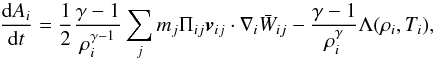 (6)where vij = vi − vj, Ti is the particle temperature, and the additional term Λ(ρi,Ti) accounts for the radiative losses of the gas, if present. In the following, simulations in which the cooling term Λ is absent from Eq. (6) are referred to as adiabatic. The expression for the AV tensor Πij is
 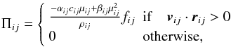 (7)so Πij is non-zero only for approaching particles. Here scalar quantities with the subscripts i and j denote arithmetic averages, ci is the sound speed of particle i, the parameters αi and βi regulate the amount of AV, and fi is a controlling factor that reduces the strength of AV in the presence of shear flows. The μij term is given by
 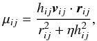 (8)where the factor η = 10-2 is included to prevent numerical divergences. To limit the amount of AV generated in shear flows, Balsara (1995) proposed the expression
 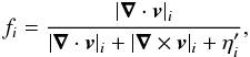 (9)where (∇·v)i and (∇ × v)i are the standard SPH estimates for divergence and curl (Monaghan 2005), and the factor
  is inserted to prevent numerical divergences. This expression for fi is effective in suppressing AV in pure shear flows, for which the condition |∇ × v|i ≫ |∇·v|i holds.
The strength of the AV in the standard SPH formulation is given by βi = 2αi and αi = const. ≡ α0, with α0 = 1 being a common choice for the viscosity coefficient (Monaghan 2005). In the following this parametrization will be referred to as the “standard” AV.
Monaghan (1997) proposed a modification to this parametrization for AV based on an analogy with the Riemann problem. In a number of test problems, results obtained using his “signal velocity” formulation are found to be equivalent or slightly improved relative to the standard AV scheme. However, this new formulation is not introduced here to avoid any further source of difference in the results produced by the SPH code, in addition to those caused by the choice of the time-dependent AV scheme parameters.
In simulations in which the gas is allowed to cool radiatively, cold gas in high density regions is subject to star formation and gas particles are eligible to form star particles. Energy and metal feedback is returned from these star particles to their gas neighbors by supernova explosions, according to the stellar lifetime and initial mass function. For a detailed description, we also refer to Valdarnini (2006).
2.2. The new artificial viscosity formulation
The standard AV formulation is successful in properly resolving shocks but at the same time generates unwanted viscous dissipation in regions of the flow that are not undergoing shocks. Morris & Monaghan (1997) proposed that the viscous coefficient should be different for each particle and left free to evolve in time under the local conditions. Following Morris & Monaghan (1997),  (10)where
  (11)is a decay timescale that regulates, by means of the dimensionless parameters ld, the time evolution of αi(t) away from shocks. The parameter αmin is the minimum value to which αi(t) is allowed to decay. The source term
  is given by
  (12)and is constructed in such a way that it increases in the presence of shocks. Following a suggestion of Morris & Monaghan (1997), the damping factor fi is inserted to account for the presence of vorticity. The scale factor
  (13)is chosen such that the peak value of αi is independent of the equation of state. The source term given in Eq. (12) is of the form proposed by Rosswog et al. (2000), and has a greater sensitivity to shocks than the original formulation. In a number of test simulations, Rosswog et al. (2000) found that appropriate values for the parameters αmax,αmin, and ld are 1.5,0.05, and 0.2, respectively.
Summary of the AV parameters used in the simulations.
From the viewpoint of the description of the fluid flow velocities, the most significant parameters are αmin and ld. Since the goal of the SPH simulations presented here is to investigate the effect of the numerical viscosity on ICM fluid flows, the set of runs are performed with the parameter αmax set to the value αmax = 1.5 (see Sect. 5.1.1), whilst a range of values are considered for the AV parameters αmin and ld. However, a lower limit to the timescale τi is set by the minimum time taken to propagate through the resolution length hi, so that the value ld = 1 sets an upper limit to the parameter ld.
The different implementations of AV used in the simulations are summarized in Table 1. In the simulations that incorporate the new time-dependent AV scheme, five different pairs of values have been chosen for the parameters (αmin,ld), while simulations in which the AV is modeled according to the standard formulation are used for reference purposes. Simulations with different AV schemes or parameters are labeled by the corresponding index of Table 1.
However, if the decay parameter ld approaches unity, the time-dependent AV scheme discussed here may fail to properly evolve the viscosity parameters αi when a shock is present. To avoid these difficulties, an AV scheme that generalizes the Rosswog et al. (2000) source term expression is proposed here. Since the implementation of the new source term equation is strictly related to the shock tube problem discussed in Sect. 5.1, the modifications to Eq. (12) are presented in Sect. 5.1 together with the shock tube tests.
3. Sample construction of simulated clusters
To investigate the effects of numerical viscosity on ICM random gas motions, a large ensemble of hydrodynamical cluster simulations was created by performing, for a chosen AV test case, SPH hydrodynamical simulations using a baseline sample consisting of eight different initial conditions for the simulated clusters. These initial conditions are those of simulated clusters that are part of a large set produced in an ensemble of cosmological simulations (see later), and these clusters are chosen at the present epoch with the selection criterion of covering a wide range in virial masses and dynamical properties. This choice was made to study, using the hydrodynamical simulations, the dependences of the ICM gas velocities on these cluster properties. The number of eight clusters was a compromise between the needs to obtain results of sufficient statistical significance and keep the computational cost to a minimum level, given the range of parameters explored.
The initial conditions of the baseline sample were constructed according to the following procedures (Valdarnini 2006), which are similar to the ones followed by Dolag et al. (2005) to construct their set of high resolution hydrodynamical cluster simulations. An N-body cosmological simulation is first run with a comoving box of size L2 = 200 h-1 Mpc. The cosmological model assumes a flat geometry with the present matter density Ωm = 0.3, vacuum energy density ΩΛ = 0.7, Ωb = 0.0486, and h = 0.7 being the value of the Hubble constant H in units of 100 km s-1 Mpc-1. The scale-invariant power spectrum is normalized to σ8 = 0.9 on an 8 h-1 Mpc scale at the present epoch.
A cluster catalog is generated by identifying clusters in the simulation at z = 0 using a friends-of-friends (FoF) algorithm to detect overdensities in excess of  . The sample comprises N2 = 120 clusters ordered according to the value of their mass M200, where
  (14)denotes the mass contained in a sphere of radius rΔ with mean density Δ times the critical density ρc.
Each of these clusters is then resimulated individually using an N-body+SPH simulation performed in physical coordinates starting from the initial redshift zin = 49. The integration is performed by first locating the cluster center at z = 0 and identifying all of the simulation particles lying within r200. These particles are then located at zin and a cube of size  , enclosing all of them, is found. A lattice of NL = 743 is set inside the cube and to each node is associated a gas particle with its mass and position; a similar lattice is then defined for dark matter particles. The particle positions are then perturbed, using the same random realization as for the cosmological simulations. The particles kept for the hydrodynamic simulation are those whose perturbed positions lie within a sphere of radius Lc/2 from the cluster center. To model tidal forces, the sphere is surrounded out to a radius Lc by an external shell of dark matter particles extracted from a cube of size 2Lc centered in the same way as the original cube and consisting of NL = 743 grid points. The particles are evolved to the present time using an entropy-conserving SPH code, described in Sect. 2.1, combined with a treecode gravity solver. Particles are allowed to have individual timesteps and their gravitational softening parameter is set according to the scaling
  , where mi is the mass of particle i. The relation is normalized by εi = 15 (mi/6.2 × 108 M⊙)1/3 kpc. The set of these individual cluster hydrodynamical simulations is then denoted as sample S2.
The whole procedure is then repeated twice more in order to generate the cluster samples S4 and S8 from cosmological simulations with box sizes L4 = 400 h-1 Mpc and L8 = 800 h-1 Mpc. The number of clusters Nm in these samples is chosen such that the mass M200 of the Nm − th cluster of sample Sm is greater that the mass M200 of the most massive cluster of sample Sm/2, and samples S8 and S4 consist of N8 = 10 and N4 = 33 clusters, respectively. The final cluster sample Sall is constructed by combining all of the samples Sm generated from the three cosmological runs.
To provide the baseline sample for the hydrodynamical simulations, eight clusters were chosen from those of sample Sall, with the selection criterion being the construction of a representative sample of the cluster dynamical states and masses.
Main cluster properties and simulation parameters of the baseline sample.
As an indicator of the cluster dynamical state, we adopt the power ratios Pr/P0. The quantity Pr is proportional to the square of the r-th moments of the X-ray surface brightness SX(x,y), as measured within a circular aperture of radius Rap in the plane orthogonal to the line of sight (Buote & Tsai 1995). Here the power ratio P3/P0, or equivalently Π3(Rap) = log 10(P3/P0), is used as an estimator of the cluster dynamical state since it gives an unambiguous detection of asymmetric structure. For a fully relaxed configuration, Πr → −∞.
For the simulated clusters of sample Sall, the power ratios are evaluated at z = 0 in correspondence of the aperture radius Rap = r200. To minimize projection effects, the average quantity  is used to estimate the cluster dynamical state, where
  is the rms plane average of the moments Pr evaluated along the three orthogonal lines of sight. Clusters of sample Sall are then sorted according to their values of
  and eight clusters are extracted from the sample. The four of them with the lowest values of among the cluster power ratio distribution are chosen and these relaxed clusters are denoted as quiescent (Q) or relaxed clusters. The remaining four are chosen with the opposite criterion of having the power ratios with the highest values among those of the distribution. These clusters are then labeled as perturbed or P clusters. Within each subset, clusters are chosen with the additional criterion of having their virial mass distribution as wide as possible. The cluster mass at r200 is used in place of the virial mass and Table 2 lists the main cluster properties and simulation parameters of the baseline sample constructed according to the above criteria.
The numerical convergence of the results is assessed by studying the dependence of the final profiles on the numerical resolution adopted in the simulations. In addition to the hydrodynamical simulations realized from the baseline sample using various AV prescriptions, a set of mirror runs with a different number of simulation particles was then performed with the aim of studying the stability of the final results against the numerical resolution of the simulations. Because of the large number of AV test simulations performed here, the stability against resolution of the simulation results for the baseline sample is investigated by comparing the chosen profiles with the corresponding ones obtained from parent simulations of lower resolution. A sufficient condition for the numerical convergence of the profiles is given by their stability against simulations performed with higher resolution. However, the approach undertaken here provides significant indications about the stability of the baseline sample and at the same time allows a substantial reduction in the amount of computational resources needed to assess numerical convergence.
The initial conditions of the mirror runs are therefore constructed using the same procedures as previously described for the baseline sample, the only difference being the number NL of grid points included inside the Lc cubes. With respect to the baseline sample, which is denoted as high resolution (HR), low (LR) and medium resolution (MR) runs are performed by setting NL = 353 and NL = 513, respectively. Table 3 lists some basic parameters. The label of each individual run is determined by combining the different labels specified in the tables.
4. Statistical measures
Here in this section we present several statistical tools with which we study the impact that the strength of AV has on the statistical properties of the turbulent velocity field u(x) of the simulated clusters. Homogeneous isotropic turbulence is commonly studied using the spectral properties of the velocity field u(x). Its Fourier transform is defined as  (15)and the ensemble average velocity power spectrum
  is given by
  (16)The energy spectrum function E(k) is then defined as
  (17)where k ≡ |k|, and the integral of E(k) is the mean kinetic energy per unit mass
  (18)In the case of incompressible turbulence, the energy spectrum follows the Kolgomorov scaling E(k) ∝ k−5/3. In contrast, the regime of compressible turbulence exhibits a large variation in the gas density and a generalized energy spectrum can be considered by introducing in Eq. (15) a weighting function u(x) → uw(x) ≡ w(x)u(x), where w(x) is proportional to some power of the density. For compressible turbulence, a natural choice is
  , in which case the integral of E(k) is just the kinetic energy density
  . As noticed by Kitsionas et al. (2009), the spectral properties of compressible turbulence are more accurately described using this weighting scheme, which allows a more accurate estimate of the power at small scales where mass accumulation occurs because of shocks. Alternatively, Kritsuk et al. (2007) demonstrated that for supersonic isothermal turbulence, a Kolgomorov scaling for the spectrum function E(k) is recovered using w(x) ∝ ρ(x)1/3. Here, we study the spectral properties of compressible turbulence using a generalized energy spectrum with density weighting given by w(x) ∝ ρ(x)1/2. This is the same as the choice adopted by Kitsionas et al. (2009) and for the energy spectrum E(k) provides a physical reference to the kinetic energy density.
To study the energy spectrum in cluster simulations, spectral quantities are constructed as follows. A cube of side Lsp with  grid points is first placed at the cluster center and hydrodynamic variables A(x) are estimated at the grid points xp according to the SPH prescription
  (19)where A(x) denotes either the components of the velocity field u(x) or the weighting function w(x).
The weighting function is set to w(x) = ρ(x)1/2/Sw, where  . This normalization choice guarantees
  , regardless of the power density exponent used in the weighting. The discrete transforms of uw(xp) are then computed using fast Fourier transforms, and an angle-averaged density-weighted power spectrum
  is generated as a function of k = |k| by binning the quantity
  in spherical shells of radius k and averaging in the bins.
As an estimator of the energy density given in Eq. (17) one can therefore use  . However, to consistently compare density-weighted power spectra extracted from different clusters and boxes it is useful to define a rescaled turbulent power spectrum as
 ![\begin{equation} E(k)=\frac{1}{L_{\rm sp} \sigma^2_v}\left [ 2 \pi k^2 \mathcal{P}^{\rm d}(k) \left (\frac{L_{\rm sp}}{2\pi} \right )^3 \right ], \label{pow.eq} \end{equation}](/articles/aa/full_html/2011/02/aa15340-10/aa15340-10-eq252.png) (20)where
(20)where  . The dimensionless form of this power spectrum allows one to compare curves of E(k) extracted from different clusters as a function of
  , where kr = |k|. The spectral properties of the gas velocity fields are studied using the density-weighted power spectrum defined according to Eq. (20), whereas volume-weighted (w = 1) spectra are considered for comparative purposes.
The main parameters used in simulations of differentresolution.
Moreover, the longitudinal and solenoidal components of the power spectrum E(k) are studied separately. To do this, the shear and compressive parts of the velocity u(x) are defined, respectively, in the k − space as 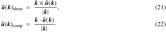 The corresponding power spectra are used to define the power spectrum decomposition, E(k) = Es(k) + Ec(k) (Kitsionas et al. 2009; Zhu et al. 2010).
In addition to the spectral properties of the velocity u(x), it is useful to investigate the scaling behavior of the velocity structure functions. These are defined by  (23)where p is the order of the function. To compute the structure functions, a random subsample of Ns particles is constructed; these particles are extracted from the set of gas particles that satisfy the constraint of being located within a distance r200 from the cluster center. For each of these sample particles s, the relative velocity difference Δu = u(xi + rsi) − u(xs) is computed for all of the gas particles i separated by a distance rsi ≤ r200, and the quantity |Δu|p is binned in the corresponding radial bin. Final averages are obtained by dividing the binned quantities by the corresponding number of pairs belonging to the radial bin.
As for the power spectrum, structure functions are computed separately for both transverse and longitudinal components. These are respectively defined as Δu ⊥ = Δu × rsi/|rsi| and Δu ∥ = Δu·rsi/|rsi|. Here the study is restricted to second-order (p = 2) structure functions. Moreover, to compare structure functions of different clusters, these are rescaled according to  and radial distances are expressed in units of r200. Density-weighted velocity structure functions are defined using the weighted field uw(x) in Eq. (23).
Finally, the energy content of the turbulent velocity field is another quantity used to investigate the dependence of the velocity field properties on the amount of AV present in the simulations. To properly consider the contribution of random gas motion to the turbulent energy budget, it is however necessary to separate from the velocity field u(x) the part due to the streaming motion. A useful approach is then to define a spatial decomposition that separates the velocity into a small-scale and a large-scale component (Adrian et al. 2000). More specifically,
 (24)where f(x − x′,H) is a shift-invariant kernel that acts as a low-pass filter, H being a filtering scale. Velocity fields are always considered here at a given time slice, so that the dependence on t is removed from Eq. (24). The small-scale turbulent velocity field
  is then defined as
  (25)This method of decomposing a turbulent velocity field is also known as Reynolds decomposition and is commonly employed in large eddy simulations (Meneveau & Katz 2000). The filtering kernel chosen here to define the large-scale velocity field is a triangular-shaped cloud function (TSC) (Hockney & Eastwood 1988). This choice is similar to that adopted by Dolag et al. (2005) when studying the ICM velocity fields, and is motivated by the compact support properties of the kernel, the TSC being a second-order scheme, which from a computational viewpoint greatly reduces the complexity of estimating the mean field velocity given by Eq. (24). The choice of the filtering scale H for the TSC spline is discussed in Sect. 6; here we note that after application of Eq. (24) to u(x), the harmonic content of the small-scale turbulent velocity field
  is defined by the condition kH ≫ 1.
5. Test simulations
We now present the simulation results obtained by applying the SPH implementation described in the previous sections to several test problems. Solutions have been provided for these problems by analytical models or independent numerical methods, and these solutions are compared with the results of the SPH runs to help validate the code and assess its performance. Section 5.1 is dedicated to the shock tube problem and Sect. 5.2 to the 3D collapse of a cold gas sphere. Both of these tests were chosen because they have been widely used in the literature and moreover they allow comparisons with previous SPH runs in which a time-dependent AV scheme was implemented.
5.1. The shock tube problem
5.1.1. Initial condition set-up and parameter calibration of the time-dependent AV scheme
The Riemann shock-tube problem is a test commonly used for SPH codes. Its main advantage is that it admits an analytical solution following the propagation of a shock wave in a medium initially at rest. Here the initial condition setup consists of an ideal fluid with γ = 5/3 initially at rest at t = 0. An interface at x = 0 separates the fluid on the right with density and pressure (ρ1,P1) = (4,1) from the fluid on the left with (ρ2,P2) = (1,0.1795). The fluid is then allowed to evolve freely and at later times a shock wave propagates toward the left, followed by a rarefaction wave and a contact discontinuity. The resulting profiles are given by the analytic solution (Rasio & Shapiro 1991).
The one-dimensional Riemann shock-tube problem is often used to test hydrodynamic codes, but the numerical results are often of limited validity because numerical effects that may arise in 3D calculations, such as particle streaming, are absent or smaller when there is only one degree of freedom. For this reason, the shock test is carried out here in three dimensions. To construct the initial conditions for the SPH runs, a cubic box of side-length unity was filled with 106 equal mass particles. Of these one million particles, 800 000 were placed in the right-half of the cube, while 200 000 were placed in the left-half. The particles in the two halves of the cube were extracted from two independent uniform glass-like distributions contained in a unit box. The two distributions had 1.6 × 10⁶ and 4 × 10⁵ particles, respectively.
These initial conditions have been chosen because they are the same as those adopted by Tasker et al. (2008, hereafter T08), in their Sect. 3.1, to study the shock tube problem. Those authors used a variety of numerical problems with known analytical solutions to compare the behavior of different astrophysical codes and their ability to resolve shocks. It is therefore of particular interest to compare the results of T08 with those obtained from the shock tube SPH simulations performed here using different AV strengths. The SPH runs were realized by imposing periodic boundary conditions along the y and z axes and the results were examined at t = 0.12. Runs with the time-dependent AV scheme have their viscosity parameters initialized to one.
Before proceeding to discuss the behavior of the shock tube tests, it is necessary to assess the validity, under different conditions, of the AV scheme introduced in Sect. 2.2. As outlined in this section, the time evolution of the viscosity parameter can be affected if very short damping timescales are imposed. To more clearly illustrate this point, it is useful to rewrite Eq. (10) using the second of the equalities of Eq. (12). The new Eq. (10) is then  (26)where
  (27)and qi is a modified source term
 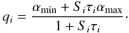 (28)Neglecting variations in the coefficients, the solution to Eq. (26) at times t > tin is given by
  (29)which indicates that αi(t) approaches the asymptotic value αmin in the absence of shocks, and αmax if a shock is present. However, for the source term qi, the condition qi ≃ αmax holds only in the shock regime Siτi ≫ 1. If this condition is not satisfied and Siτi ≲ 1, the peak value αpeak of αi(t) will be smaller than αmax. In particular, αpeak will depend on the chosen value of the decay parameter ld. This dependence of αpeak on ld is absent for strong shocks, but for mild shocks introduces the unwanted feature that for short decay timescales (ld → 1) the peak value of αi(t) at the shock front might be below the AV strength necessary to properly treat shocks.
Application of the SPH code implemented according to the AV scheme described in Sect. 2.2 to the shock tube problem with the initial condition setup studied here, shows that at the shock front location the peak in the AV parameter ranges from unity to ~0.2 for ld = 1. Previous numerical tests (Morris & Monaghan 1997; Rosswog et al. 2000) showed that for this shock tube problem there is good agreement with the exact results using ld = 0.2, and at the shock front the peak in the viscosity parameter is then approximately ~0.6−0.7.
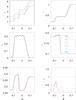 |
Fig. 1 Results at t = 0.12 from the shock tube test for 3D SPH runs with different AV parameters. The profiles are projected along the shock front. From top to bottom are plotted: density, velocity, and thermal energy (left column); pressure, entropy, and viscosity parameter (right column). The solid black line represents the analytical solution, while lines with different styles and colors are the profiles of the SPH runs with different AV parameters. Different runs are labeled according to Table 1 and the relationship with the corresponding profiles is illustrated in the entropy panel. In the density panel, profiles of different runs have been shifted vertically to more clearly illustrate their relative differences. |
To maintain the same shock resolution capabilities in those cases studied using short timescales with ld = 1, a correction factor ζ is introduced so as to compensate in the source term qi for the smaller values of Siτi with respect to the small ld regimes. This is equivalent to considering a higher value for αmax, so that in Eq. (28) αmax is substituted by αmax → ζαmax. The calibration of the correction factor ζ is achieved by requiring that for the current shock tube problem, the SPH runs with AV decay parameters ld > 0.2 should have at the shock front the same value αpeak as that for the ld = 0.2 case, i.e. αpeak ~ 0.6−0.7 for ld > 0.2. This choice guarantees that the viscosity parameter reaches the correct size at the shock front, but away from it quickly decays according to the chosen value of ld. After several tests, it has been found that the choice ζ = MAX((ld/0.2)0.8,1) yields satisfactory results and all the numerical tests shown in this paper incorporate in the source term in Eq. (12) the modification 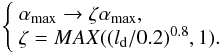 (30)Note that the validity of this setting was established for the shock strength of the shock tube problem considered here; nonetheless the results of the other tests indicate that this parametrization is appropriate to make the peak value of the viscosity parameter at the shock location independent of the chosen value for the decay parameter ld.
5.1.2. Results
The results of the shock tube tests are shown in Figs. 1 and 2. In each panel, different profiles refer to runs with different AV parameters. The solid line is the analytical solution, which exhibits a shock front at x = −0.095 and a contact discontinuity at x = −0.033. The profiles shown in Figs. 1 and 2 can be compared with the corresponding Figs. 2 and 3 of T08.
The fixed AV simulation is in good agreement with the GADGET2 run of T08, although a closer view of the density profile in the proximity of the shock front in Fig. 2 shows post-shock ringing features that are absent in T08. This happens because close to the shock the amount of AV generated by the code allows particle interpenetration. To avoid post-shock oscillations in the density, T08 explicitly made the choice of setting the viscosity parameter in the GADGET2 run to ArtBulkVisc = 2, whereas here the fixed AV run was performed with the viscosity parameter α set to unity. The post-shock oscillations in velocity are very similar in amplitude and behavior to the ones produced by the GADGET2 run of T08, and similarly for the glitch in pressure at the contact discontinuity. The spike in thermal energy and entropy at the contact discontinuity is caused by the initial discontinuity in the density profile, which has been left unsmoothed at the beginning of the simulation. These features are also present in T08, although here the height of the spikes is a bit smaller.
The profiles of the simulations in which a time-dependent AV scheme was implemented show a behavior very similar to those of the fixed AV run. The post-shock oscillations in the density have a tendency to be amplified as the AV scheme uses shorter decay timescales, but the effect is minimal. This can be seen in the top left panel of Fig. 1, in which the density profiles have been shifted vertically to illustrate the effect more clearly. The differences in the other profiles as a function of the AV coefficients are very small, with the post-shock entropy being the quantity with the strongest dependence and the smallest values being those of the AV runs with the lowest viscosity parameter (ld = 1). Finally, the radial profiles of the time-dependent artificial viscosity parameters α are consistent with the discussion of Sect. 2.2: their peaks are located approximately at the shock front and their post-shock radial decay is faster for those AV runs with the shortest decaying timescales.
To summarize, the simulations of the shock tube problem performed with the SPH code presented here using the standard AV scheme show results in good agreement with the analytic solution and with the ones obtained by other authors using a similar initial condition setup and set of parameters. The profiles of the runs with a time-dependent AV scheme agree well with those of the fixed AV run, thus indicating that the shock resolution properties are comparable to those of the standard AV scheme, but have a reduced AV strength elsewhere.
5.2. Collapse of a cold gas sphere
The Riemann shock-tube test of the previous section illustrates the ability of the code to resolve discontinuities, but the shock strengths produced by the test are much smaller than those that develop during the gravitational collapse of astrophysical objects. A more stringent test for SPH codes in which gasdynamics is modeled including self-gravity is therefore to study a 3D collapse problem. The test used by Evrard (1988) follows in time the adiabatic collapse of a gas sphere. This test has been widely used by many authors (Hernquist & Katz 1989; Steinmetz & Mueller 1993; Davé et al. 1997; Wadsley et al. 2004; Springel 2005; Vanaverbeke et al. 2009; Wetzstein et al. 2009) as one of the standard tests for SPH codes. The shock strength that develops during the collapse is comparable to that of the Navarro & White (1993) self-similar collapse test.
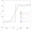 |
Fig. 2 A closer view of the shock front of the density profiles displayed in the top left panel of Fig. 1. |
The gas cloud is spherically symmetric and initially at rest, with mass M, radius R, and density profile  (31)The gas obeys the ideal gas equation of state with γ = 5/3 and the thermal energy per unit mass is initially set to u = 0.05GM/R. The chosen time unit is the cloud free-fall timescale
 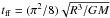 1 and the SPH simulations are performed using units for which G = M = R = 1. The cloud begins to collapse under its own gravity and the gas in the core is heated until the growth of pressure is sufficient for the infalling material to bounce back and a shock wave then propagates outwards. Most of the kinetic energy is converted into heat at the epoch of maximum compression of the gas, which occurs at t ~ 1.1.
The initial conditions for the simulations are constructed by stretching the radial coordinates of a glass-like uniform distribution of N = 88 000 equal mass particles contained within a sphere of unit radius. Radial coordinates are transformed according to the rule r → r′ = r3/2, so as to generate the density profile of Eq. (31). The particle smoothing lengths are adjusted according to Eq. (2) with Nsph = 50 neighbors and the gravitational softening length is taken as εg = 0.02. This choice for the simulation parameters allows one to compare the test calculations performed here with the results presented for the same collapse problem by Wetzstein et al. (2009) in their Sect. 7.1.
Figure 3 shows the radial dependence at t = 0.9 of the spherically averaged profiles for density, pressure, radial velocity, and time-dependent viscosity. The solid line represents the high-resolution 1D PPM simulation of Steinmetz & Mueller (1993), which for practical purposes can be considered as being an exact solution. The differences between the profiles with different AV parameters are minimal and the post-shock radial decay of the viscosity parameters is in accord with the expectation of the model. The profiles of the SPH runs are consistent with previous findings (Springel 2005; Wetzstein et al. 2009) and reproduce the overall features of the PPM solution, with some differences at the shock front, which at this epoch is located at r ~ 0.18. To illustrate these differences, Fig. 4 shows a closer view of the density and entropy profiles in the proximity of the shock front.
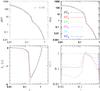 |
Fig. 3 Results at t = 0.9 for the adiabatic collapse of a cold gas sphere. Clockwise from the top left panel: radial density profiles of density, pressure, viscosity parameter α and radial velocity. The black solid lines are the results of the 1D PPM calculation of Steinmetz & Mueller (1993). SPH runs with different AV parameters are labeled in the same way as in the shock tube test panels of Fig. 1. |
A feature common to all of the runs is a significant amount of pre-shock entropy generation. This is inherent to the AV implementation of the SPH code, which near the bounce is switched on by the strong convergence of the flow, thus generating dissipation (Wadsley et al. 2004). Different settings of the AV parameters are clearly reflected in the code’s ability to model shocks and compressions that in turn generate the corresponding differences in the pre-shock entropy profiles. All of the simulations share the basic attribute of having a shock front located outside the position indicated by the reference PPM entropy profile. The location of the shock front has a weak dependence on the implemented AV settings, the time-dependent AV runs with the shortest decay timescales (runs AV4 and AV5) being the closest to the PPM reference position. Moreover, the fixed AV run overpredicts the entropy peak, whilst the other time-dependent AV simulations are in rough agreement with the PPM one. Finally, the post-shock entropy profile of all the runs is below the corresponding reference PPM profile.
The density and entropy panels of Fig. 4 can be compared with Figs. 7 and 8 of Wetzstein et al. (2009). For the chosen parameter settings, the AV1 run corresponds to the Wetzstein et al. (2009) model with δa = 5 and α⋆ = 0.1, whilst AV2 corresponds to the δa = 2, α⋆ = 0.1 model. A comparison shows that the results presented here share some common properties with those of Wetzstein et al. (2009), but at the same time there are also several differences. For instance, compared to the reference PPM entropy profile, pre-shock entropy production and a lower entropy level behind the shock is common to both of the tests. However, in Wetzstein et al. (2009), pre-shock heating for the time-dependent AV models occurs at radii larger than for the fixed AV run and the differences in the entropy profiles (as well as in the density) for different AV runs are here reduced yet further.
It is difficult to ascertain the origin of the different behavior of the two codes in the proximity of the shock front, given also that the differences in the corresponding profiles are not dramatic. However, the SPH formulation implemented in the two codes differs in several aspects, so that even results produced for the same test problem and the same initial conditions might be different. The thermal evolution of the gas is followed here according to an entropy-conserving scheme, while in the Wetzstein et al. (2009) code it is the specific internal energy that is integrated. Moreover, unlike Wetzstein et al. (2009), in Eq. (3) the equation of motion incorporates the terms related to the presence of smoothing length gradients. The reader is referred to Springel & Hernquist (2002) for a thorough discussion of the relative differences between simulation results produced using the two SPH formulations.
To summarize, for the test problem considered the results presented in this section agree with previous findings and validate the code, as well as showing its capability to properly model shocks that develop during the collapse of self-gravitating objects. In accordance with the results of Sect. 5.1.2, profiles extracted from simulations with a time-dependent AV scheme exhibit a behavior that is very similar to the corresponding ones for the fixed AV model, thus showing shock resolution capabilities analogous to those of the standard AV scheme for these models. Finally, the peaks of the viscosity parameters at the shock front appear almost independent of the chosen value of the AV decay parameter ld, thereby supporting the proposed parametrization given in Eq. (30).
6. Cluster simulations
We now study the impact of numerical viscosity on the ICM velocity field of simulated clusters using the statistical tools presented in Sect. 4. The purpose of the analysis is also to obtain useful indications concerning the numerical constraints necessary to adequately describe turbulence in simulations of the ICM using SPH codes.
6.1. Velocity power spectra
Fourier spectra extracted from hydrodynamical simulations are expected to exhibit a dependence on both the simulation resolution and the hydrodynamical method used in the simulations. Resolution issues are usually debated in a dedicated section to assess the stability of the simulation results. Here, however, the interpretation of the results is strictly related to the resolution employed in the simulations, so the two arguments are discussed together.
To measure the velocity Fourier spectra of the simulated clusters, a cube of side length Lsp is placed at the cluster center, the latter being defined as the location where the gas density reaches its maximum value. As described in Sect. 4, Fourier transforms of the density-weighted velocity field are evaluated by first estimating interpolated quantities at the cube grid points and then performing a 3D FFT of the sampled values. The choice of the cube side length Lsp and the number of grid points is however limited by several arguments that strongly constrain the possible choices.
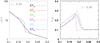 |
Fig. 4 The same as in Fig. 3, radial profiles of density and entropy are shown in the proximity of the shock front. |
At variance with studies of supersonic turbulence using hydrodynamical simulations (Kitsionas et al. 2009, herefater K09; Price & Federrath 2010), here the gas distribution is driven by gravity and because of the Lagrangian nature of the SPH code, the bulk of the particle distribution is located in the central cluster regions. For the cluster simulations presented here, about half of the cluster mass at the present epoch is contained within a radius of ~r200/3. Therefore, to minimize this aspect of the resolution effects, the size of the cube should be kept as small as possible, but in this case most of the large-scale modes will be missed in the spectral analysis, in particular, those modes corresponding to the merging and accretion processes of the cluster substructure. As a compromise between these two oppositing needs, the side-length of the cube is set to Lsp = r200 (the scaling Lsp ∝ r200 being chosen to consistently compare velocity spectra extracted from different clusters).
The choice of the number of grid points in the cube or, equivalently, of the grid spacing Lsp/Ng, depends on the effective SPH resolution of the simulations. In SPH, the smallest spatially resolvable scale is set by the values of the gas smoothing lengths hi. As already outlined, because of the Lagrangian nature of SPH simulations, the gas particle number density increases in high-density regions and this in turn implies a subsequent decrease in the gas smoothing lengths hi. If in these regions the SPH spatial resolution becomes higher than the grid resolution of the cube, SPH kernel interpolation at the cube grid points will appear in the k − space as a extra power at the highest wave number permitted by the grid. This effect was noticed by K09 and can be avoided provided that the cube grid spacing is chosen to be suitably small. For the HR cluster simulations, values of the gas smoothing lengths hi in the cluster cores range from hi ~ 20 kpc for the most massive clusters down to hi ~ 5 kpc for the least massive ones. Similar values for the grid spacing are obtained by setting Ng = 128 grid points along each of the spatial axis of the cube. However, the number of cube grid points cannot be made arbitrarily high because of the need to avoid undersampling effects in the estimate of SPH variables at the grid points. As a rule of thumb, the number Ng should not exceed  , with Np being the number of SPH particles.
Finally, when calculating the velocity power spectra non-periodicity effects should be taken into account by adopting a zero-padding technique (Vazza et al. 2009). However, application of this method to the clusters presented here requires some care since the choice of the cube side length Lsp is dictated by the previous constraints so that a cube of volume  occupies at the cluster center ~1/4 of the volume of a sphere of radius r200 with its origin being identical to that of the cube. Hence, a power estimate based on the non-periodicity assumption would likely underestimate the velocity power spectrum at wavenumbers ~π/Lsp, in particular for clusters undergoing a major merging event. The procedure adopted here should then provide a more accurate indication of the spectral behavior of the ICM velocity field at spatial scales of about the cube size.
Having chosen the cube parameters, velocity power spectra have been evaluated at the present epoch for the ensemble of simulated clusters constructed by collecting simulations of the the cluster HR baseline sample performed with different AV prescriptions. The resulting spectra are shown in Figs. 5 to 8 and provide a quantitative comparison between statistical properties of the longitudinal and solenoidal velocity field spectral components for clusters simulated with different AV settings and different dynamical states. Each panel in the figures corresponds to an individual cluster and the curves shown in the panels are the velocity power spectra extracted from simulations of the considered cluster realized using different AV parameters.
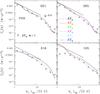 |
Fig. 5 Compressive components of the density-weighted velocity power spectra (20) are shown at z = 0 as a function of the dimensionless wavenumber |


A first conclusion to be drawn from the spectra shown in the figures is that, for a given cluster and power spectrum component, at large scales the velocity power spectra do not exhibit systematic differences between different AV runs and therefore the effects of numerical viscosity can be considered negligible on these scales. Moreover, dissipative effects in the kinetic energy are less important for those runs in which the parameter settings of the time-dependent AV scheme correspond to the shortest decay timescales for the viscosity parameter α(t). At high wavenumbers, the power spectra of the AV5 runs have larger amplitudes than those of the standard AV runs (AV0) by a factor of ~2 and in certain cases even by a factor of ~10 ( see, for example, the longitudinal power spectrum of cluster 110 of the relaxed subsample). These behaviors are shared by the velocity power spectrum components of all of the simulated clusters and because of the sample size can be considered systematic.
The use of Fourier spectra allows one to study in a quantitative way the scale dependency of dissipative effects due to numerical viscosity. All of the spectra exhibit a maximum at  , at spatial scales of ~r200/2. This is a key signature in the power spectra of the ICM velocity field, in which merging and accretion processes driven by gravity at cluster scales are the primary sources of energy injection into the ICM. Similar findings were obtained by Vazza et al. (2009), who measured the velocity power spectrum of simulated clusters in cosmological simulations using the AMR Eulerian code ENZO.
Spectra of runs with different AV settings begin to deviate at wavenumbers  . This indicates that for the present simulation resolution (HR) the effects of numerical viscosity on the formation of eddies due to Kelvin-Helmholtz instabilities generated by substructure motion (Takizawa 2005; Subramanian et al. 2006) become significant at spatial scales ldiss = π/kd ~ r200/10 ~ 100−200 kpc, in accordance with the behavior of the velocity structure functions (see later). The generation of these instabilities leads to the development of turbulent motions that, as expected, are stronger in those runs with the lowest numerical viscosity. There are no large differences seen between the shape of the spectra extracted from clusters in different dynamical states. However, the power spectra of relaxed clusters, in comparison with the spectra of the dynamically perturbed clusters, show a certain tendency to flattening at large scales and smaller amplitudes at the smallest cube wavenumber.
For comparative purposes, each panel shows for the considered case the volume-weighted velocity power spectrum of the standard AV run. The behavior of the other volume-weighted spectra reflects the similarities seen in the corresponding density-weighted spectra of simulations with different AV settings and for the sake of clarity these spectra are not shown in the panels.
At large scales, volume-weighted and density-weighted spectra do not show significant differences, with few expections such as the longitudinal power spectra of cluster 105 of the perturbed subsample. Variations in the behavior of density-weighted spectra and volume-weighted spectra are expected to appear at smaller scales, when gas density gradients become significant. We note, however, that there are no systematic differences between density and volume-weighted spectra as a function of wavenumber versus the cluster dynamical state and/or power spectrum decomposition.
At high wavenumbers, density-weighted spectra in certain cases can have values below those of volume-weighted spectra. This is interpreted as a resolution effect, which becomes stronger as runs with lower resolution (MR or LR) are considered. As already outlined, the gas distribution is driven by gravity and because of the Lagrangian nature of the SPH code, for wavelength modes approaching the grid spacing the contribution of low density regions that are undersampled becomes dominant. This effect is not present in all of the clusters because it is strongly dependent on the degree of gas inhomogeneity, which in turn depends on the individual cluster dynamical history.
Although the aim of the paper is to assess the effectiveness of the time-dependent AV scheme in reducing the numerical viscosity in SPH cluster simulations, the velocity power spectra presented here can nevertheless be used to obtain useful indications about the description of turbulence in the ICM when SPH simulations are used.
Below the driving scales  , the longitudinal component of the energy spectra exhibit an approximate power-law behavior close to the Kolgomorov scaling that extends down to dissipative scales. These features are not shared by the solenoidal component of the spectra. To study the behavior of the shearing part of the spectra, it is useful to introduce the ratio Ψ(k) ≡ Ec(k)/(Ec(k) + Es(k)), which measures as a function of the wavenumber the fractional contribution of the longitudinal velocity power spectrum component. This ratio lies in the range Ψ(k) ~ 0.3−0.5 at large scales and rises above
  , the latter is defined as approximately the wavenumber at which the bending in Ψ(k) occurs. While the ratio at large scales can be understood in terms of fully developed turbulence, the rise in Ψ(k) at small wavenumbers is a consequence of the steep decrease in the shearing part of the spectra in this range of scales, which is interpreted here as a resolution effect. This behavior shows that a fundamental issue to be addressed is the resolution dependence of the velocity power spectra extracted from the simulations.
K09 and Price & Federrath (2010) studied supersonic isothermal turbulence using both SPH and Eulerian-based codes. Both groups reach the conclusion that differences in the simulation results are mainly due to the resolution used, with dissipative effects specific to the codes confined at high wavenumbers. Equivalent results in the measured velocity power spectra are obtained using an equivalent number of resolution elements N for each direction in space in simulations with different codes. For example, SPH simulations with N3 = 5123 particles would give comparable results to those obtained using the same number of grid cells in Eulerian simulations.
Exploiting this correspondence, one can then interpret the dependence of the velocity power spectra on resolution effects using the results of Federrath et al. (2010), who studied interstellar turbulence using a FLASH code with up to N3 = 10243 cell elements. From the simulations, the authors (see their Sect. 6) measure in the extracted Fourier spectra E(k) a rise in Ψ(k) starting at k ~ 40 ~ N/26, which they explain as a resolution effect. Basically, this happens because the number of computational elements needed to accurately resolve rotational modes is larger than that necessary to describe longitudinal modes, for which only one degree of freedom is present. In fact, longitudinal modes appear to be clearly described down to k ~ N/10, implying that there is a difference in the resolution scale of a factor of ~three.
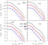 |
Fig. 9 Shearing components of the density-weighted velocity power spectra are shown at z = 0 for the runs of the relaxed test clusters as a function of the wavenumber. As in the previous figures, different line styles are for different AV runs. In each panel runs with different resolution are displayed with different line thickness. For the sake of clarity, not all of the AV runs are plotted and runs with different AV parameters have been equispaced from top to bottom by a factor of 10. To more clearly illustrate the wavenumber dependence, spectra have been computed here using |

Application of these results to the present simulations suggests that the solenoidal part of the spectra is barely resolved in the HR runs, with a resolution scale 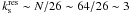 , whilst the longitudinal component is resolved down to
  . To corroborate these findings, Fig. 9 shows the solenoidal component of the density-weighted velocity power spectra versus the wavenumber for simulations of different resolution for the subsample of relaxed clusters. All of the spectra show a well-defined tendency towards shallower slopes as the simulation resolution is increased, with a reduction of the dissipative range towards higher wavenumbers. This spectral behavior is also partly explained by the larger number of matter clumps that are now resolved at small scales as the mass resolution is increased, thus adding power to the spectra at high wavenumbers. At large scales, a slight decrease in the amplitude of the spectra can occur because of resolution effects, as the resolution is increased clumps of matter accreting at r ~ r200 survive more easily therefore reducing the amount of turbulence injected into the medium via ram-pressure stripping mechanisms. This effect can be seen in Fig. 9 for clusters 011 and 019, for which the large-scale part of the spectra decreases as the resolution is increased. Moreover, in certain cases there is a plateau in the spectra at high wavenumbers that is removed as the resolution is increased.
Figure 10 shows the ratio Ψ(k), for the same test runs. Although there are large cluster-to-cluster variations, cluster 110 offers nevertheless a clear example of how  shifts towards higher wavenumbers as the resolution is increased. This dependence on the numerical resolution also confirms that the predominance of the compressive components in the velocity power spectra in not due to the presence of shocks at small scales, with the primary injection mechanisms occurring at cluster scales. However, the estimates of inferred from the application of other simulation results might be too pessimistic. From Fig. 10, it can be seen that for clusters 013 and 110, Ψ(k) is stable down to
  . These values are a factor of ~two higher than those estimated from previous scalings.
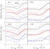 |
Fig. 10 The ratio of the longitudinal to total velocity power spectra are shown at z = 0 for runs of the relaxed test clusters as a function of the wavenumber. The line coding is the same as in the previous figure; runs with different AV parameters have been equispaced from top to bottom by a factor 0.2. |
Similar underestimates are found for the dependence of the dissipative scale set by numerical viscosity on the numerical resolution. According to K09, length scales defined by the condition k > N/32 are affected by dissipative mechanisms specific to the code. This implies that dissipative effects here should start acting from  , whereas the spectral behavior indicates that at least down to
  there are no significant differences between spectra extracted from runs with different AV settings.
We need to address the dependence on the numerical resolution of the dissipative scales identified from the spectral behavior of the velocity power spectra. Longitudinal power spectrum components are more helpful to this study because for these spectra, numerical resolution effects are less severe than for the solenoidal components. As in Fig. 9, a comparison of the behavior of the longitudinal part of the density-weighted velocity power spectra for simulations of different resolutions, shows that the dissipative wavenumber  scales approximately as N, suggesting that to resolve eddies down to length-scales of the order of galaxy-sized objects (~50 kpc) simulations would be required with at least N3 = 2563 gas particles. However, the spatial range of ldiss derived from the spectra of Figs. 5–8 is in rough agreement with that expected using analytical models (Subramanian et al. 2006) to estimate the coherence velocity field length-scale associated with minor mergers in clusters. Moreover, Maier et al. (2009) presented an Eulerian-based AMR code with subgrid modeling for turbulence at unresolved scales. The authors studied the evolution of turbulence in cluster simulations and argue that most of the turbulent energy is injected into the medium at length scales of ~125−250 h-1 kpc (cf. their Fig. 6). This consistency between different independent estimates of the characteristic turbulent length scales therefore suggests that for the HR runs, spectral features due to dissipative effects might be of physical origin rather than due to numerical resolution effects.
 |
Fig. 11 Transverse (S ∥ ) and longitudinal (S ⊥ ) second-order normalized velocity structure functions at z = 0 for HR runs of the perturbed test clusters as a function of r/r200. |
To summarize, the application of previous findings (Kitsionas et al. 2009; Federrath et al. 2010; Price & Federrath 2010) to the simulations presented here produces several discrepancies in the resolution dependence of characteristic scales, which appear less severe here than those found by these authors. A clarification of these issues clearly has to await simulations with much higher resolution, although it appears that physical differences in the problems considered might play a role. For instance, here is gravity the driving force that dominates the dynamics of the collapsed object, thereby that creating, owing to the adaptative nature of the SPH codes in space, a “scale dependence” in resolution as one moves outwards from the cluster center. As a consequence, the effective resolution of the simulations performed here might be higher than that estimated using simple scaling arguments.
However, these results indicate that the present simulation resolution is clearly inadequate to fully describe the spectral behavior of the ICM velocity field, therefore raising the question of what is the minimum number of particles needed to adequately resolve turbulence in SPH simulations. This is strictly related to the minimum spatial scale that must be resolved in the velocity Fourier spectra. Requiring for the study of rotational motion at least one order of magnitude in spectral resolution, implies that N3 = 5123 particles are needed for a correct description of turbulence in SPH simulations of the ICM. Taking into account the previous caveats, the same results could be obtained using N3 = 2563 particles.
In addition to spectral analysis, the scale dependence of dissipative effects can be studied using the velocity structure functions that provide information in physical space about the velocity field self-correlation. In particular, the second-order structure function  is complementary to Figs. 5–8 for obtaining informations about the effects of numerical viscosity on the velocity field statistics. Evaluating the structure functions is a computationally demanding task since the number of pairs scales approximately as
  . The choice of the subsample size Ns is a compromise between the needs of adequately sampling the structure functions and reducing the computational cost. The parallel and transverse second-order structure functions were calculated here by setting Ns = Ngas/8, corresponding approximately to ~5 × 10⁹ pairs for the HR runs. This choice for Ns is found to give convergent results when tested against higher values. We note that a uniform random number extraction of Ns particles from the simulation particles does not correspond to an approximately uniform sampling in space, as the bulk of the gas particles (~1/2) are concentrated within distances ≲r200/3 from the cluster center.
The parallel and transverse second-order velocity structure functions are shown in Fig. 11 for the HR runs using volume-weighted velocities. All of the functions exhibit an increase with increasing pair separation  , thereby showing how turbulence in the ICM is substained by motions on cluster scales. For two of the clusters (1 and 5), the radial dependence is approximately a power law, a result which can be taken as indicative of a scaling range, although this issue needs to be clarified with simulations of much higher resolution.
Assuming that the structure functions produced by the standard AV runs are the reference profiles, structure function profiles extracted from the runs with a time-dependent AV scheme at small scales deviate significantly from the reference profile. The deviation increases as  decreases and becomes wider as the decaying viscosity parameter ld approaches unity. This behavior clearly shows the effectiveness of the new numerical viscosity scheme in reducing the viscous damping of velocity away from shocks, and therefore of the code being more able to follow the development of turbulent motion. Profiles of the structure functions extracted from simulations of lower resolution are noisier than the profiles presented here but preserve the basic features shown in Fig. 11, hence supporting the validity of these arguments.
Structure functions derived using a density-weighted velocity are shown in Fig. 12. They exhibit the same behavior as for the volume-weighted functions but with a much shallower radial dependence. This is due to the adopted weighting scheme, for which the contribution of those pairs located in high density regions is enhanced with respect to the volume-weighted functions. This preferentially happens at small scales because in SPH codes most of the particles are located in high density regions. Finally, a comparison with the spectra shown in Figs. 5–8 shows an approximate correspondence between the length scales (~r200/10) at which dissipative effects become significant.
6.2. Average radial profiles
Measurements of the average radial profiles of thermodynamic variables, such as density or temperature, extracted from spatially resolved X-ray observations allow one to probe ICM properties and test the predictions of cosmological cluster simulations. This is achieved by comparing the observed ICM profiles with those extracted from mock X-ray data. It is therefore important to examine in SPH cluster simulations the impact of numerical viscosity on the radial profiles of the variables considered.
To do this, the final radial profiles of the gas entropy 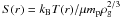 are shown in Fig. 13 for the simulated clusters of the relaxed subsample. As in Figs. 5–8, each panel corresponds to an individual cluster and within each panel different curves are for runs with different AV settings. To compare the entropy profiles of different clusters, the entropy has been normalized to
 ![\begin{equation} S_{200}=\frac{1}{2}\left [\frac{2 \pi}{15} \frac {G^2 M_{200}}{f_bH}\right]^{2/3}, \label{entr.eq} \end{equation}](/articles/aa/full_html/2011/02/aa15340-10/aa15340-10-eq407.png) (32)where fb = Ωb/Ωm is the global baryon fraction.
(32)where fb = Ωb/Ωm is the global baryon fraction.
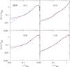 |
Fig. 13 Final radial entropy profiles for the HR runs of the relaxed test clusters. Gas entropy is defined as |
![\hbox{$S_{200}=\frac{1}{2}\left [\frac{2 \pi}{15} \frac {G^2 M_{200}}{f_{\rm b}H(z)}\right]^{2/3}$}](/articles/aa/full_html/2011/02/aa15340-10/aa15340-10-eq409.png)
Discussion of the dependence of the final profiles on the AV scheme used in the simulations is restricted here to the entropy only, since both density and temperature profiles exhibit quite similar behavior. A feature common to all of the entropy profiles is the relatively small scatter between those profiles extracted from runs for a given cluster with different strengths of the numerical viscosity. The variations in the entropy profiles caused by the AV implementation appear to be confined to the inner cluster regions (~10% of r200). As already outlined in the Introduction, we need to investigate the amount of entropy present in cluster cores (Agertz et al. 2007; Wadsley et al. 2008; Mitchell et al. 2009). Viscous damping of random gas motion is expected to be lower in low-viscosity runs, thereby increasing fluid mixing and possibly the accretion at the cluster center of gas with higher entropy, with a subsequent rise of the entropy floor in the core.
The profiles of Fig. 13 illustrate that the amount of gas mixing due to numerical viscosity is not significant, although there is a certain tendency for the core entropy to be influenced by the AV strength of the simulation. For instance, cluster 11 exhibits a large difference of ~5 between the core entropy S(rc = 0.01r200) of run AV0 and that of run AV4. For two other clusters (12 and 110), the entropy profiles of the low-viscosity runs increase moderately with respect to that of the standard AV run as the radial coordinate decreases, with central differences being smaller than a factor of ~two. Finally, there is one cluster (19) for which S(rc) of run AV4 is below that of run AV0. This behavior is shared by the entropy profiles of the perturbed cluster subsample and it indicates that the amount of entropy mixing in cluster cores induced by numerical viscosity effects is modest or quite negligible.
The stability of the results is assessed in Fig. 14 by contrasting for the same test clusters the entropy profiles of simulations with different resolution. In each panel, the profiles of only three AV runs are plotted (AV2, AV4, and AV5) to avoid overcrowding. From Fig. 14, it can be seen that there is little variation between the entropy profiles of runs performed with the same AV settings but with different resolution. In the AV5 test case, for several clusters the profiles of the HR runs show some deviations at small distances from those with lower resolution. Interpretation of this difference as a systematic effect due to inadequate resolution requires some care, however, since it is absent in the profiles of the other AV runs. Moreover, even for the test case AV5, in one cluster (110) the core entropy S(rc) does not vary with the simulation resolution.
To summarize, the reliability of the entropy profiles of simulated clusters with respect to variations in the simulation resolution is supported by the profiles of Fig. 14, for which one sees the lack of any systematic dependence of S(rc) with varying numerical resolution. This indicates that the profiles of Fig. 13 can be reliably used to draw the conclusion that in SPH simulations the amount of entropy present in cluster cores due to numerical viscosity effects can be considered negligible. The smallness of AV effects in determining the core entropy of simulated clusters therefore indicates that the discrepancy, which originates at the cluster centers between SPH and grid-based Eulerian codes in the produced entropy profiles of adiabatic simulations, is inherent to the method itself rather than being a problem of the AV scheme implemented in the SPH codes. In particular, the lack of significant AV effects indirectly confirms that the primary source of the entropy discrepancy between the two hydrodynamical approaches resides in the treatment of flow discontinuities in SPH simulations (Agertz et al. 2007).
To overcome these difficulties, Price (2008) and Wadsley et al. (2008) proposed to add an explicit diffusion term in the SPH thermal energy equation to smooth the discontinuities present in the thermal energy at the fluid interfaces. The introduction of this diffusion term leads to a certain amount of gas mixing and in turn to an establishment of an entropy core in simulated clusters (Wadsley et al. 2008), which appears to qualitatively agree with that produced by Eulerian codes. However, generation of vorticity associated with fluid instabilities is severely affected by viscous damping due to numerical viscosity. Using a suite of 2-D numerical tests, Price (2008) showed that the treatment of Kelvin-Helmholtz instabilities can be greatly improved in SPH codes provided that the hydrodynamic equations are reformulated so as to include thermal diffusion as well as variable AV coefficients. It would then be interesting to reinvestigate for the same test sample presented here the growth of central entropies using SPH simulations in which the hydrodynamic equations have been modified by adding an artificial thermal energy dissipation term.
The radial profiles α(r) of the viscosity parameters are shown in Fig. 15 for the relaxed subsample. For each cluster, only the profiles of runs AV2 and AV5 are shown, the radial behavior of the profiles for the other AV runs being intermediate between the two. Within each panel, the profiles of the AV test cases are accompanied by the viscosity profiles extracted from the corresponding low and medium resolution runs. This is to help us estimate the stability of the profiles to variations in the numerical resolution of the simulations. From the figure, it can be seen that for a given AV setting there is little scatter between the profiles extracted from runs with different resolutions, with some differences close to the shock front that are not however significant. The profiles of the perturbed cluster subsample are similar to those shown here, but with a wider scatter because of the different dynamical histories of these clusters. The radial behavior of the profiles is in agreement with expectations: we note that for two clusters (19 and 110), the peak values αpeak of α(r) at the shock front for the run AV5 are significant smaller than those for run AV2. This is not the case for the peak values of run AV4 (not shown here), which are similar to those of run AV2, indicating therefore that for weak shocks (say αpeak ≲ 0.3) the peak value of the viscosity parameter is influenced by the floor value αmin of the gas particles ahead of the shock.
One of the most important aspects in which viscous damping of random gas motion is expected to influence ICM properties, is in the ICM energy budget. To investigate the impact of numerical viscosity on the energy content of the ICM, it is necessary however to properly distinguish in the velocity field u(x) the contribution of bulk motions from the small-scale chaotic parts. Following Dolag et al. (2005), a turbulent velocity field can then be defined by subtracting from u(x) a local mean velocity ⟨ u(x) ⟩ . According to Eq. (25), the latter is defined by using a TSC window function to interpolate gas density and velocities at the grid points of a cubic mesh with grid spacing H. The mean velocity ⟨ u(x) ⟩ is defined by averaging over the gas particles that belong to the grid cell; subtraction of the filtered velocity from the velocity field u(x) is expected to remove the contribution of large-scale motions and leave a velocity with spectral content dominated by those wavenumbers for which kH ≫ 1. The choice of the filtering scale H is somewhat arbitrary: Dolag et al. (2005) found that a mesh spacing of the order of ~30 kpc yields consistent results; in agreement with the choices of Sect. 6.1, the scaling H ∝ r200 is adopted here, allowing the velocity field of clusters of different masses to be compared in a self-similar way. The choice of H is a compromise between the needs of removing the contribution of bulk flow motions to u(x) as much as possible and the constraints imposed by the numerical resolution of the simulation for which values of H that are too small lead to an undersampling of local estimates. These effects are expected to become significantly lower by requiring at least Nc ~ 102 gas particles in the cube cells. From this constraint, the allowed range of the grid spacing H can be estimated using the average gas density radial profiles. For the clusters presented here, ρ/ρc ~ 5 at the cluster radius r200 and for the HR runs this translates into a range of values for H between ~740 kpc for the most massive clusters down to ~350 kpc for the least massive ones.
These filtering scales are too large to effectively remove bulk motion components from the velocity field u(x). As a compromise, the contribution of turbulent energy can be investigated by restricting the study to the inner parts of the cluster. At the radius r ~ r200/2, the cluster gas densities lie around ρ/ρc ~ 30 and the range for H is now between ~400 kpc and ~180 kpc, which corresponds to H ~ r200/5, when rescaled to the cluster radius r200. Although this choice does not completely remove from the laminar flow patterns present in the ICM, it should filter out most of the contribution to u(x). Vazza et al. (2009) studied the development of turbulence in the ICM using the adaptative grid AMR cosmological code ENZO and argued that for their simulated cluster the ICM velocity field at length scales ≳ 300 kpc is dominated by laminar flows. Moreover, the turbulent energy density radial profiles constructed from a filtered field using a length scale of H/2 do not show appreciable differences from those derived here using H as a filtering scale.
 |
Fig. 15 As in Fig. 9, final profiles of the viscosity parameter α are shown for the runs of the relaxed test clusters with different AV parameters and resolution. In each cluster panel the profiles have been plotted without any shifting between the various cases. |
To consistently compare our simulation results with those of Vazza et al. (2009), the radial density profiles are constructed using the same definitions. The thermal energy density is defined as Eth = 3kBT(r)ρg(r)/2μmp, where T(r) is the mass-weighted gas temperature, kB is the Boltzmann constant, μ = 0.6 is the molecular weight, mp is the proton mass, Ekin = ρgu2/2, and  are, respectively, the kinetic and turbulent energy density. The total energy density is defined as Etot = Eth + Ekin. All the quantities with a radial dependence are estimated by averaging over a collection of values; these are calculated according to the SPH prescription given in Eq. (19) at a set of grid points uniformly spaced in angular coordinates and lying on the surface of a spherical shell, located at distance r from the cluster center. The energy density profiles constructed in this way are shown in Fig. 16 for the clusters of the perturbed subsample. The profiles have been rescaled in units of
  and for the sake of clarity for each cluster only the profiles extracted from the runs of two AV test cases (AV0 and AV4) are shown. The corresponding ratios Eturb/Etot are shown in Fig. 17.
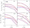 |
Fig. 16 Final energy density radial profiles constructed from the HR runs of the dynamically perturbed test clusters. Each panel shows: the profile of the thermal energy density Eth = 3kBT(r)ρg(r)/2μmp, the kinetic energy density profile Ekin = ρgu2/2 and the turbulent one |
A first conclusion to be drawn from the radial behavior of the profiles is the significant impact on the ratio Eturb/Etot of the numerical viscosity scheme adopted in the simulation. Because of the suppression of the viscous damping of random gas motion, for the runs AV4 the ratio Eturb/Etot at any radial distance is higher than that of the corresponding runs AV0 by a factor ranging between ~30% and ~100%. The ratio is nearly constant for the cluster 005 (~8%) and 016 (~10% ) and increases from ~2% to ~5% for cluster 105. Finally, for cluster 001 it decreases (~10% at r = r200/100) as r increases (~5% at r = r200/2). A similar behavior is present for the profiles of the relaxed cluster subsample.
These findings indicate the lack of any systematic dependence of the ratio Eturb/Etot on the cluster radial distance and illustrate the sensitivity of the turbulent energy density profile on the dynamical history of the individual cluster. To extract statistically meaningful results about the contribution of random gas motion to the ICM energy budget, it is then necessary to use a very large simulated sample (say ≳ 100 clusters, see, e.g., Piffaretti & Valdarnini 2008).
It is difficult to assess the consistency of the profiles presented here with those obtained by Vazza et al. (2009), since the results indicate large cluster-to-cluster variations among the individual turbulent energy density profiles and in Vazza et al. (2009) the profile is shown for only one cluster. However, the authors argue that, for their cluster, the turbulent energy budget is smaller by a factor ~5−6 than previous SPH results. The ratio Eturb/Etot lies here in the range between a few percent and ~5−10%, and similar values for this ratio are quoted by Vazza et al. (2009). Moreover, a visual inspection shows a strong similarity between the profiles of cluster 105 and those derived by Vazza et al. (2009) for their simulated cluster (Fig. 6, bottom right). As already stressed in Sect. 6.1, a proper study of turbulence in the ICM using an SPH code awaits simulations of much higher resolution than those presented here, although these results are encouraging and support the view that SPH simulations can be used to investigate this topic, provided that the numerical viscosity effects are properly treated and the medium is adequately resolved.
It is important to investigate the impact of the numerical viscosity scheme on the cluster mass bias estimated from simulations. The relative importance of different mass bias components has been studied in detail (Piffaretti & Valdarnini 2008) using a large set of N-body/SPH simulations of galaxy clusters. Apart from the bias caused by the use of observational quantities, such as spectroscopic temperatures, and those induced by assuming specific models for the measured profiles, it was found that mass underestimates are dominated by the hydrostatic equilibrium assumption and the absence in the Jeans equation for the mass of pressure support terms due to random gas motions. In particular, for relaxed clusters the mass bias due to these terms increases with the distance r from the cluster center and can be as high as ~5−10% for r ranging between r2500 and r200. Given that the importance of galaxy clusters as cosmological probes relies on the use of accurate mass estimators, it is therefore important to estimate in the Jeans equation the dependency of these gas motion terms on numerical viscosity.
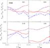 |
Fig. 17 Ratio of the turbulent to the total pressure, Ptu/Ptot ≡ Eturb/Etot, for the profiles of Fig. 16. Additionally, for the same test runs, are shown (thin lines) the ratios of the “velocity” pressure to the total one : |
![\hbox{$P_{\sigma}/ \left[P_{\sigma}+P_{\rm th}\right]= \frac{1}{3}\sigma^2(r) /\left[ kT(r)/\mu m_{\rm p} +\sigma^2(r)/3 \right]$}](/articles/aa/full_html/2011/02/aa15340-10/aa15340-10-eq459.png)
To achieve this, the relative importance of the velocity pressure terms is quantified by constructing the radial profile of 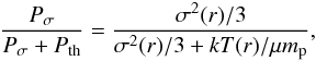 (33)where σ(r) is the rms gas velocity dispersion. The latter is evaluated at the same radial shells used to evaluate the energy density profiles. In analogy with Eq. (33), a relative turbulent pressure term can be defined, Pturb/Ptot, for which Pturb/Ptot ≡ Eturb/Etot. The quantities Pσ/(Pσ + Pth) can then be directly compared with the turbulent-to-total energy density ratios and these are shown in Fig. 17 as thin lines. For the four test clusters, the ratio increase with the radial distance r and Pσ/(Pσ + Pth) ~ 10−20% at r = r500 ~ 0.6r200, while at the same distance Pσ/(Pσ + Pth) ~ 10% for the relaxed subsample.
This range of values for the contribution of random gas motions to the total pressure is in accordance with the estimates extracted from previous simulations (Rasia et al. 2006; Nagai et al. 2007a; Piffaretti & Valdarnini 2008; Lau et al. 2009). Moreover, the profiles of Pσ/(Pσ + Pth) show a weak dependency on the numerical viscosity scheme used in the simulations. Differences between the profiles are significant in the cluster cores, but at r = r500 the profiles of runs AV0 differ by a few per cent from those of runs AV4, indicating therefore that pressure terms due to random gas motions are already estimated to good approximation in SPH simulations in which a standard AV scheme is implemented. The physical consequences of this result will be discussed in the conclusions, but it is worth discussing the origin of the different radial behavior of the ratio Pσ/(Pσ + Pth) with respect to that of Eturb/Etot.
The rms gas velocity σ(r) is defined as 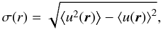 (34)where the field velocity u(r) is calculated according to the SPH prescription at the grid points of the spherical shell and brackets denote averages performed over the set of points. This definition is in accordance with the procedures used to compute the energy density profiles; however, the gas velocity dispersion calculated following the standard definition, i.e. by averaging over the gas particles contained within the shell of radial coordinate r and thickness Δr, does not differ significantly from that obtained using Eq. (34). The different radial behavior of the rms gas velocity dispersion σ(r) from that of the local velocity field
  can be ascribed to the different procedures adopted to compute the two velocities, which in turn define the two fields.
Because of the filtering procedures, the latter is dominated by the small-scale random gas motion with a coherence length scale ~200−300 kpc. For the rms gas velocity σ(r), the contribution of laminar infall motion is not removed but mixed with that of the turbulent motion. Therefore, while the local velocity field can be properly defined as a turbulent velocity field (Vazza et al. 2009), the dispersion σ(r) is just a measure of the gas velocity variance at the scale r. This is why the ratio Eturb/Etot does not show a well-defined dependence on radius, while σ(r) increases with r as the streaming motion due to accretion from the infalling material becomes progressively more important. A similar viewpoint is discussed by Zhu et al. (2010, see also Maier et al. 2009), who studied the generation of vorticity fields by means of of hydrodynamic simulations to measure the level of turbulence in the intergalactic medium.
To summarize, the notion of turbulent pressure support, which accounts for the X-ray mass bias when assuming hydrostatic equilibrium for the ICM, is somewhat misleading at large cluster radii because the velocity terms missed in the Jeans equation are dominated by the streaming motion of the infalling material, and in the cluster outskirts the local turbulent velocity field becomes progressively less important when compared to those terms.
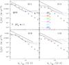 |
Fig. 18 As in Fig. 7, compressive components of the density-weighted velocity power spectra are shown at the present epoch for the cooling HR runs of the relaxed cluster subsample. |
6.3. Simulations with cooling and star formation
The discussion of the previous section attempted to investigate the effects of numerical viscosity on ICM properties when the gas evolution of the cluster is driven by relatively simple physics, in which gravity is the sole driver of structure formation. However, a realistic modeling of the physics of the ICM must incorporate the possibility that the gas cools radiatively, turning cold dense clumps of gas into stars. Moreover, energy and metal feedback that follows from supernova explosions should also be considered. Hydrodynamical simulations in which these physical processes have been taken into account (Muanwong et al. 2002; Tornatore et al. 2003; Valdarnini 2003; Kay et al. 2004; Nagai et al. 2007b) have shown that there is substantial agreement between the predicted ICM properties, such as the temperature profiles, and the corresponding measurements, though significant discrepancies still remain (Borgani & Kravtsov 2009). In particular, the model overpredicts the star mass fraction, which is found in simulations to be a factor ~2−3 higher than that estimated from observations. This is the so-called “overcooling” problem, for which several explanations have been proposed (Borgani & Kravtsov 2009), although there is not yet a definitive solution.
An improvement in the AV scheme used in the SPH code is expected to significantly modify the ICM properties of the simulated cooling clusters. To investigate these effects, the analyses of the previous sections are repeated here using the same set of cluster samples, but in the simulations the physical modeling of the gas now includes radiative cooling and star formation, as well as energy and metal feedback from supernovae (Valdarnini 2006). Our analysis of the results of the simulations will not replicate the thorough discussion of Sects. 6.1 and 6.2, but only the most important results will be presented from the viewpoint of AV when cooling is incorporated into the simulations.
When applying the spectral analysis of Sect. 6.1 to the velocity fields produced by radiative simulations, a striking feature that emerges from the spectral behavior of the transformed fields is the presence at small scales of a driving source that injects turbulence into the ICM. The density-weighted velocity power spectra for the compressive components of the relaxed cluster subsample are shown in Fig. 18 and exhibit a spectral behavior that stops decaying at  and thereafter is nearly flat at higher wavenumbers, or even grows as in the case of cluster 110. These features are in sharp contrast to the corresponding spectra of Fig. 7 for the adiabatic runs and are clearly induced by the presence of cooling.
Previous investigations have considered generation of turbulence in cluster cores to occur either by means of the interaction of the ambient ICM with buoyantly rising bubbles created from AGN jet activities (Churazov et al. 2001; Brüggen & Kaiser 2002), or induced by orbital motion of galaxies (El-Zant et al. 2004; Kim 2007). The origin of turbulence is interpreted here as being due to the development of dense compact cool gas cores in the inner cluster regions. These are characterized by the presence of central gas densities for which ρ/ρc ~ 104, about a factor ~10 higher than in the corresponding adiabatic runs. Following Fujita et al. (2004b) and Fujita (2005), the interaction of these dense cool cores with the bulk gas motion of the surrounding ICM leads then to hydrodynamical instabilities and the production of turbulence. That the origin of the turbulent injection resides in the interaction of the cluster core with the ambient medium is confirmed by the radial dependence of the viscosity parameters (Fig. 19), which exhibit a rising ramp in the proximity of the cluster centers because of the weak shocks that form near the core. Owing to resolution issues, it appears difficult to assess in a quantitative way the small-scale behavior of the derived spectra, although it seems unlikely that this effect should not be confirmed in simulations in which the spectra are adequately resolved, as similar features are already present in the low resolution runs MR and LR. For the same reason, no attempt is made here to extract any possible dependence of the spectra on the numerical viscosity of the simulations, as there is a large scatter at small scales between spectra of a given cluster but with different AV settings.
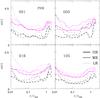 |
Fig. 19 As in Fig. 15, final profiles of the viscosity parameter α are shown for the cooling runs of the perturbed test clusters with different AV parameters and resolution. |
These results provide strong support however for the plausibility of models in which radiative cooling in the cluster cores is compensated by turbulent heating of the ICM (Fujita et al. 2004b; Fujita 2005). This scenario is observationally motivated by the lack of resonant scattering from X-ray spectra (Churazov et al. 2004) as well as by the constraints on diffusion processes extracted from measured iron abundance profiles (Rebusco et al. 2006; David & Nulsen 2008), which indicate how the outward diffusion in cluster cores of iron must be driven by turbulent gas motion. Heating of the ICM was investigated by Dennis & Chandran (2005), who constructed a set of analytical models in which radiative cooling is locally balanced by dissipation of turbulent motion, entropy mixing via turbulent diffusion, and heat conduction. To compensate for radiative losses, both the heating rates from turbulent diffusion and dissipation are in general important for establishing thermal equilibrium. The local turbulent heating rate from turbulent dissipation is given by 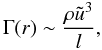 (35)where l is the driving length scale and to balance radiative losses estimates derived from simple models (Dennis & Chandran 2005; David & Nulsen 2008) require
  km s-1. This range of values is smaller than that found here in the central cluster regions for the local velocity
  of the simulated clusters by roughly a factor ~50%, showing therefore that analytical models might overestimate the amount of entropy mixing necessary to achieve thermal balance in cluster cores. We note, however, that in massive clusters a viable mechanism for the dissipation of turbulence is collisionless damping (Brunetti & Lazarian 2007), hence for these clusters the contribution of the heating rate in Eq. (35) to the ICM thermal balance might be overestimated. Finally, as indicated by Fig. 19, a certain amount of shock heating is present to reduce the effects of cooling in the core.
High levels of turbulence in cluster cores may also have a significant impact on the stability of cold fronts. These structures are interpreted as contact discontinuities produced when gas of different entropy is brought into contact (Markevitch & Vikhlinin 2007). In the sloshing scenario (ZuHone et al. 2010, and references therein), this happens because of the interaction of the cool core gas with substructures falling through the main cluster. Accordingly, cold fronts are created as the subsonic sloshing of the central gas causes the encounter of gas flows from different directions. However, cold fronts are prone to disruption by hydrodynamical instabilities (ZuHone et al. 2010; Roediger et al. 2010) and it is unclear whether the level of turbulence found in the cluster cores of the simulations shown here can be reconciled with the presence of cold fronts seen in many clusters. This is beyond the scope of this paper and clearly deserves further investigation. In particular, hydrodynamic simulations that incorporate a proper modeling of the physical viscosity of the ICM can be used to investigate the stability of cold fronts in the sloshing scenario (ZuHone et al. 2010). The derived constraints on the ICM viscosity should then permit us to address the viability of turbulent heating models in balancing radiative losses.
The radial profiles of the energy density ratios, together with the relative pressure terms, are shown in Fig. 20. These profiles are the analog for the cooling runs of those of Fig. 17 for the nonradiative case. A comparison between the two figures shows that at r ≲ 0.1r200 there are no large variations in the Eturb/Etot profiles, with the exception of cluster 105. This follows because at r ≲ 0.1r200 the steepening in Eturb is accompanied by a corresponding steepening in Etot, so that the ratio Eturb/Etot retains a profile approximately similar to that of the nonradiative case. The same behavior is found for the radial profiles of Pσ/(Pσ + Pth), which show a very little dependence on the AV strength of the simulations at r ≳ 0.1r200. These results also hold for the relaxed subsample. Because the physical description of the ICM in these simulations is more realistic than in the nonradiative case, these results provide support for the findings of the previous section, indicating that numerical viscosity effects have little impact on the bias of hydrostatic mass estimates. A similar conclusion holds for the entropy profiles, which are shown in Fig. 21 and exhibit very little scatter between runs with different AV settings. This is interpreted as a consequence of galaxy formation processes so that the small amount of entropy mixing found in the cluster cores for the adiabatic runs has now been removed.
The radial profiles of the gas mass fraction fg(<r) = Mgas(<r)/Mcl(<r) are shown in Fig. 22 for the perturbed test clusters. The quantity fg(<r) is an increasing function of the radius r, as the amount of cooled gas subject to star formation is a decreasing function of radius because of the dependence of the cooling function on the gas density. At r = r500 ~ 0.6r200, the value of fgas is practically independent of the AV scheme used in the simulations, whereas at inner radii it is difficult to extract meaningful information about the dependence of fg(<r) on the implemented AV scheme. For instance, at radii r ≲ 0.1r200 the highest values of fg(<r) are those of runs AV5 for clusters 001, 005, and 105. The lowest values of fgas are found at r ≲ 0.1r200 for the standard viscosity runs AV0 in the case of clusters 005 and 105.
According to the new AV formulation, the turbulent heating of the ICM is higher because of the suppression of viscous damping of the random gas motion. This in turn implies that the star formation efficiency is lower because of the higher level of turbulent pressure, and that at a given radius the quantity fgas should exhibit higher values for those runs where the AV is reduced. The scatter between the profiles of Fig. 22 does not allow us to reach firm conclusions about this dependence, indicating that a very large simulated sample is needed to clarify this issue. Finding a statistically significant dependence of fgas on the AV scheme used in the simulations would support the viewpoint that turbulence might play a significant role in solving the overcooling problem, as suggested by Zhu et al. (2010).
To summarize, the role of numerical viscosity in simulations that incorporate radiative cooling is significant in cluster cores, where the strength of turbulence driven by hydrodynamical instabilities is amplified far more strongly than the nonradiative case, but is negligible in establishing the shape of the ICM profiles at cluster radii r ≳ 0.1r200. Results from the previous section support the view that simulations with a much larger number of gas particles (≳ 2563) are necessary to consistently investigate the first of these issues, while at radii r ≳ 0.1r200 the stability of the ICM profiles presented here appears quite robust.
7. Summary and conclusions
We have presented the results of hydrodynamical SPH simulations developed to investigate the role of the SPH numerical viscosity scheme in determining ICM properties of simulated galaxy clusters. The standard AV formulation of SPH has been modified according to the proposal of Morris & Monaghan (1997), where each particle has its own viscosity parameter α(t) that evolves in time under the local shock conditions. This time-dependent AV scheme has the main advantage of properly reducing the amount of AV present in the fluid in regions far from shocks, with respect the standard AV scheme where the corresponding parameters are held constant throughout the simulation domain. The new time-dependent AV scheme has been implemented in an SPH code and several numerical tests have been performed to assess the validity of the code and its shock resolution capabilities. The chosen tests were the Riemann shock tube problem and 3D collapse of a cold gas sphere. Both of these problems have been widely studied in the literature, and the results of previous simulations provide reference profiles against which to compare the profiles extracted from the simulations produced here.
For the tests considered, the results of simulations performed using the standard AV scheme are in good agreement with previous findings, showing the validity of the code. To investigate the impact of the time-dependent AV scheme in reducing numerical viscosity effects, for a given test case a set of SPH simulations that incorporate the new AV formulation has been constructed, in which the runs use the same initial conditions but differ in the settings of the AV parameters that control the time evolution of the individual viscosity coefficients. The results of these simulations show profiles that are very similar to those produced by the fixed AV runs, indicating that the new AV scheme has shock resolution capabilities similar to those of the standard one and at the same time a reduced AV far from the shocks. Moreover, the time evolution of the viscosity parameter α(t) is consistent with theoretical expectations and at the shock front the coefficients reach peak values that are nearly independent of the chosen AV settings. Finally, in the cold gas sphere, the entropy profiles of the time-dependent AV runs exhibit reduced pre-shock heating at the shock front and closer agreement with the reference 1D PPM numerical solution.
Having established the reliability of the code and the effectiveness of the new AV formulation, the impact of AV on ICM properties of simulated clusters has been investigated by extracting results from a large ensemble of hydrodynamical cluster simulations. The ensemble has been constructed by collecting samples of simulated clusters, each of the samples being produced by performing simulations for the same set of cluster initial conditions but using a different setting of the AV parameters in the SPH code. The baseline cluster sample with which the simulation ensemble has been constructed consisted of eight clusters chosen from a cosmological simulation ensemble with cluster virial masses ranging from M200 ~ 5 × 10¹³ h-1 M⊙ up to M200 ~ 6 × 10¹⁴ h-1 M⊙, the selection criterion being that of constructing a representative sample of cluster dynamical states and masses. The dependence of the results on the numerical resolution of the simulations has been tested by constructing a set of mirror ensembles in which the only difference in the cluster simulations with respect to the corresponding one of the reference ensemble was in the number of simulation particles. Moreover, the ensembles of adiabatic cluster simulations have been replicated following the same prescriptions but with the gas being allowed to cool radiatively and being subject to star formation. The final outcome of these procedures is a set of hydrodynamical cluster simulations which allow the dependence of ICM gas velocities on the AV scheme used in the simulations to be studied in a systematic way. Here, the main results are summarized.
The velocity Fourier spectra of the simulated clusters have certain features in common that allow several conclusions to be drawn about the generation of random gas velocities. All of the spectra exhibit a maximum at the smallest spectral cube wavenumber, showing that merging and accretion processes driven by gravity at cluster scales are the primary sources of energy injection into the ICM. The spectra manifest their dependence on dissipative effects at length scales ldiss ~ r200/10 ~ 100−300 kpc, below which the less dissipative spectra are those extracted from runs in which the AV settings correspond to the shortest decay timescale for the viscosity parameter α(t). The range of values for ldiss appears to be in accordance with previous findings (Subramanian et al. 2006; Maier et al. 2009), suggesting that the detected spectral features are not an artifact caused by resolution effects. These behaviors are consistent with those derived from the structure function radial profiles and are common to all of the clusters, regardless of the dynamical state of the cluster.
Spectral decomposition into a transverse and a longitudinal part allows the resolution dependence of the spectra to be studied and useful insights to be obtained into the resolution requirements which must be fulfilled in order to adequately resolve turbulence in SPH simulations of galaxy clusters. The longitudinal component of the velocity power spectrum Ec(k) is found to exhibit an approximate Kolgomorov scaling over nearly a decade, whilst the shearing part Es(k) has a much steeper fall off. In analogy with previous findings (Federrath et al. 2010), this behavior is interpreted as a resolution effect, as the number of computational elements needed to adequately resolve rotational motion is higher than that necessary for longitudinal modes, where only one degree of freedom is present. Using scaling arguments derived from previous simulations (K09; Price & Federrath 2010) a number of N ~ 5123 gas particles is then needed to adequately describe turbulence driven spectra in SPH simulated clusters. However, this estimate might be too pessimistic, as the SPH resolution is not constant but increases with the particle density toward the cluster center, although it appears unlikely that less than ~2563 particles can be used to describe Es(k) over a decade.
Entropy is a fundamental thermodynamic variable and the corresponding average radial profiles have been chosen to investigate the dependence of the final ICM thermal properties on the AV scheme used in the simulations. As a function of the AV simulation parameters for the entropy profiles of a given cluster, a very small scatter is found with the largest differences in most cases being ≲50% within radial distances r ≲ 0.1r200. The weak dependency of the entropy profiles on the AV parameters of the simulations indicates that the amount of entropy mixing in cluster cores due to numerical viscosity effects can be considered negligible. As a consequence, the discrepancy between SPH and Eulerian codes in the core entropy produced in adiabatic cluster simulations can be primarily related to the treatment of fluid discontinuities in the SPH formulation, rather than to AV effects.
At variance with the entropy profiles, the radial behavior of the turbulent energy density profile Eturb(r) exhibits a significant dependence on the chosen AV scheme. There is an increase in the turbulent-to-total energy density ratio as less dissipative AV runs are considered, with the largest variations occurring at r ≲ 0.1r200. The range of values for the ratio Eturb/Etot is in accordance with previous findings obtained using the AMR Eulerian code ENZO (Vazza et al. 2009) and provides support for the view that differences between results extracted from SPH and grid based codes can be reconciled using an adequate number of simulation particles in SPH simulations and properly treating the AV.
A striking result is the lack of any significant dependence at large cluster radii of the rms gas velocity σ(r) on the AV parameters used in the simulations. As this quantity dominates in the Jeans equation the mass correction terms to the hydrostatic equilibrium equation, it follows that numerical viscosity effects can be considered negligible in determining the corrections to the hydrostatic X-ray cluster mass estimates. Hence, previous SPH simulations in which the AV is treated according to the standard formulation, already provide numerically reliable estimates for the X-ray mass bias (Piffaretti & Valdarnini 2008). One important consequence of this result is that the agreement between the measured hydrostatic X-ray and weak lensing mass ratio (Mahdavi et al. 2008; Zhang et al. 2008, 2010) with the X-ray mass bias predicted by simulations (Zhang et al. 2010), strongly supports the already outlined scenario (Piffaretti & Valdarnini 2008), in which the level of non-thermal pressure present in the ICM is not significant and the gas physics outside cluster cores is described well by the current SPH simulations.
In simulations that incorporate radiative cooling, a significant feature is the presence in the inner cluster regions of a much higher level of turbulence, which is produced by the hydrodynamical instabilities generated by the interaction of the compact cool core with the ambient medium. Moreover, the range of values of the local turbulent velocity is in accordance with the constraints required by the turbulent heating model to balance radiative losses (Dennis & Chandran 2005).
To address the viability of the turbulent heating model in a quantitative way, a proper treatment would be needed of the small-scale fluid instabilities that develop near the cluster cores. This requires the use of simulations that have a much larger number of particles and at the same time incorporate in the SPH equations the thermal diffusion terms that were previously proposed (Price 2008; Wadsley et al. 2008) to correctly model fluid instabilities in SPH. The latter is particularly relevant in order to reliably estimate the radial profile of the local velocity  , which is an important factor in establishing the local balance between the turbulent heating rate and radiative losses (Dennis & Chandran 2005). These simulations will still miss some basic ingredients of the physics describing the thermodynamics of the ICM in cluster cores, in particular the effects of to thermal conduction, heating from AGN jets, physical viscosity, and instabilities driven by the presence of magnetic fields (Parrish et al. 2010). Nonetheless, the information provided by these simulations will probably shed light on the role played by turbulence in establishing the observed bimodal distribution of cluster core entropies (Pratt et al. 2010) and the morphological distinction between cool-core and non cool-core clusters.
To summarize, the results presented here indicate that turbulence is likely to play a significant role in some open issues of ICM physics, such as the cooling flow and the overcooling problems. To properly investigate these issues, it would be necessary however to further improve the hydrodynamic SPH equations, so as to correctly treat fluid discontinuities, and to use a much larger number of particles. For a given test cluster, a comparison between the results produced by these simulations and those extracted from simulations obtained using an Eulerian AMR code is likely to give interesting insights into the physical problem as well as the numerical framework.
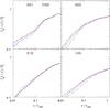 |
Fig. 22 Final radial profiles of the gas fraction fg(<r) = Mgas(<r)/Mcl(<r) are shown for the HR cooling runs of the perturbed cluster subsample in units of the cosmic value |

Note that this time normalization is the same as that of Hernquist & Katz (1989) and differs by a factor of  from that of Evrard (1988) and by π2/8 with respect to that adopted by Steinmetz & Mueller (1993).
Acknowledgments
The author is grateful to R. Brunino for kindly providing the glass-like initial conditions with which the numerical tests of Sect. 5.1 were done and to M. Steinmetz for providing the PPM solution used in Sect. 5.2. S. Kitsionas and F. Vazza are also gratefully acknowledged for helpful comments which clarified some of the issues discussed in Sect. 6.
References
- Adrian, R. J., Christensen, K. T., & Liu, Z. C. 2000, Exp. Fluids, 29, 275 [Google Scholar]
- Agertz, O., Moore, B., Stadel, J., et al. 2007, MNRAS, 380, 963 [NASA ADS] [CrossRef] [Google Scholar]
- Balsara, D. 1995, J. Comp. Phys., 121, 357 [Google Scholar]
- Berger, M. J., & Colella, P. 1989, J. Comp. Phys., 82, 64 [NASA ADS] [CrossRef] [Google Scholar]
- Borgani, S., & Kravtsov, A. 2009, Advance Science Letters (ASL), Special Issue, Computational Astrophysics, in press [arXiv:0906.4370] [Google Scholar]
- Brüggen, M., & Kaiser, C. R. 2002, Nature, 418, 301 [NASA ADS] [CrossRef] [PubMed] [Google Scholar]
- Brunetti, G., & Lazarian, A. 2007, MNRAS, 378, 2345 [Google Scholar]
- Buote, D. A., & Tsai, J. C. 1995, ApJ, 452, 522 [NASA ADS] [CrossRef] [Google Scholar]
- Churazov, E., Brüggen, M., Kaiser, C. R., Böhringer, H., & Forman, W. 2001, ApJ, 554, 261 [NASA ADS] [CrossRef] [Google Scholar]
- Churazov, E., Forman, W., Jones, C., Sunyaev, R., & Böhringer, H. 2004, MNRAS, 347, 29 [NASA ADS] [CrossRef] [Google Scholar]
- Colella, P., & Woodward, P. R. 1984, J. Comp. Phys., 54, 174 [Google Scholar]
- Davé, R., Dubinski, J., & Hernquist, L. 1997, New Astr., 2, 277 [NASA ADS] [CrossRef] [Google Scholar]
- David, P. D., & Nulsen, P. E. J. 2008, ApJ, 689, 837 [NASA ADS] [CrossRef] [Google Scholar]
- Dennis, T. J., & Chandran, B. D. G. 2005, ApJ, 622, 205 [NASA ADS] [CrossRef] [Google Scholar]
- Dolag, K., Bartelmann, M., & Lesch, H. 2002, A&A, 387, 383 [NASA ADS] [CrossRef] [EDP Sciences] [Google Scholar]
- Dolag, K., Vazza, F., Brunetti, G., & Tormen, G. 2005, MNRAS, 364, 753 [NASA ADS] [CrossRef] [Google Scholar]
- El-Zant, A. A., Kim, W.-T., & Kamionkowski, M. 2004, MNRAS, 354, 169 [NASA ADS] [CrossRef] [Google Scholar]
- Evrard, A. E. 1998, MNRAS, 235, 911 [Google Scholar]
- Federrath, C., Roman-Duval, J., Klessen, R. S., Schmidt, W., & Mac Low, M.-M. 2010, A&A, 512, A81 [NASA ADS] [CrossRef] [EDP Sciences] [Google Scholar]
- Frenk, C. S., White, S. D. M., Bode, P., et al. 1999, ApJ, 525, 554 [NASA ADS] [CrossRef] [Google Scholar]
- Fryxell, B., Olson, K., Ricker, P., et al. 2000, ApJS, 131, 273 [NASA ADS] [CrossRef] [Google Scholar]
- Fujita, Y. 2005, ApJ, 631, L17 [NASA ADS] [CrossRef] [Google Scholar]
- Fujita, Y., Suzuki, T. K., & Wada, K. 2004a, ApJ, 600, 650 [NASA ADS] [CrossRef] [Google Scholar]
- Fujita, Y., Matsumoto, T., & Wada, K. 2004b, ApJ, 612, L9 [NASA ADS] [CrossRef] [Google Scholar]
- Hernquist, L., & Katz, N. 1989, ApJS, 70, 419 [NASA ADS] [CrossRef] [Google Scholar]
- Hockney, R. W., & Eastwood, J. W. 1988, Computer simulation using particles (Bristol: Hilger) [Google Scholar]
- Iapichino, L., & Niemeyer, J. C. 2008, MNRAS, 368, 1089 [NASA ADS] [CrossRef] [Google Scholar]
- Jeltema, T. E., Hallman, E. J., Burns, J. O., & Motl, P. M. 2008, ApJ, 681, 167 [NASA ADS] [CrossRef] [Google Scholar]
- Kay, S. T., Thomas, P. A., Jenkins, A., & Pearce, F. R. 2004, MNRAS, 355, 1091 [NASA ADS] [CrossRef] [Google Scholar]
- Kim, W.-T. 2007, ApJ, 667, L5 [NASA ADS] [CrossRef] [Google Scholar]
- Kitsionas, S., Federrath, C., Klessen, R. S., et al. 2009, A&A, 508, 541 [NASA ADS] [CrossRef] [EDP Sciences] [Google Scholar]
- Kravtsov, A. V., Klypin, A. A., & Khokhlov, A. M. 1997, ApJS, 111, 73 [NASA ADS] [CrossRef] [Google Scholar]
- Kritsuk, A. G., Norman, M. L., Padoan, P., & Wagner, R. 2007, ApJ, 665, 416 [NASA ADS] [CrossRef] [Google Scholar]
- Lau, E., Kravtsov, A. V., & Nagai, D. 2009, ApJ, 705, 1129 [NASA ADS] [CrossRef] [Google Scholar]
- Mahdavi, A., Hoekstra, H., Babul, A., & Henry, J. P. 2008, MNRAS, 128 [Google Scholar]
- Maier, A., Iapichino, L., Schmidt, W., & Niemeyer, J. C. 2009, ApJ, 707, 40 [NASA ADS] [CrossRef] [Google Scholar]
- Markevitch, M., & Vikhlinin, A. 2007, Phys. Rep., 443, 1 [NASA ADS] [CrossRef] [EDP Sciences] [Google Scholar]
- Meneveau, C., & Katz, J. 2000, Ann. Rev. Fluid Mech., 32, 1 [Google Scholar]
- Mitchell, N. L., McCarthy, I. G., Bower, R. G., Theuns, T., & Crain, R. A. 2009, MNRAS, 395, 180 [NASA ADS] [CrossRef] [Google Scholar]
- Monaghan, J. J. 1997, J. Comput. Phys., 136, 298 [NASA ADS] [CrossRef] [MathSciNet] [Google Scholar]
- Monaghan, J. J. 2005, Rep. Progr. Phys., 68, 1703 [NASA ADS] [CrossRef] [Google Scholar]
- Monaghan, J. J., & Gingold, R. A. 1983, J. Comput. Phys., 52, 374 [NASA ADS] [CrossRef] [Google Scholar]
- Morris, J. P., & Monaghan, J. J. 1997, J. Comput. Physics, 136, 41 [Google Scholar]
- Muanwong, O., Thomas, P. A., Kay, S. T., & Pearce, F. R. 2002, MNRAS, 336, 527 [NASA ADS] [CrossRef] [Google Scholar]
- Nagai, D., Vikhlinin, A., & Kravtsov, A. V. 2007a, ApJ, 655, 98 [NASA ADS] [CrossRef] [Google Scholar]
- Nagai, D., Kravtsov, A. V., & Vikhlinin, A. 2007b, ApJ, 668, 1 [NASA ADS] [CrossRef] [Google Scholar]
- Navarro, J. F., & White, S. D. M. 1993, MNRAS, 265, 271 [NASA ADS] [Google Scholar]
- Norman, M. L. 2005, in Adaptive Mesh Refinement – Theory and Applications. (Berlin, New York: Springer), ed. T. Plewa, T. Linde, & V. G. Weirs, Lect. Notes Comput. Sci. Eng., 41, 413 [Google Scholar]
- Norman, M. L., & Bryan, G. L. 1999a, in The Radio Galaxy Messier 87 (Berlin: Springer-Verlag), ed. H.-J. Röser, & K. Meisenheimer, Lect. Notes Phys., 530, 106 [Google Scholar]
- Norman, M. L., & Bryan, G. L. 1999b, in Numerical Astrophysics, ed. S. M. Miyama, K. Tomisaka, & T. Hanawa (Boston: Kluwer), Astrophysics and Space Science Library, 240, 19 [Google Scholar]
- O’Shea, B. W., Bryan, G., Bordner, J., et al. 2005a, Introducing Enzo, an AMR Cosmology Application, in Adaptive Mesh Refinement – Theory and Applications, ed. T. Plewa, T. Linde, & V. G. Weirs (Berlin, New York: Springer), of Lecture Notes in Computational Science and Engineering, 41, 341 [Google Scholar]
- O’Shea, B. W., Nagamine, K., Springel, V., Hernquist, L., & Norman, M. L., 2005b, ApJS, 160, 10 [NASA ADS] [CrossRef] [Google Scholar]
- Parrish, I. J., Quataert, E., & Sharma, P. 2010, ApJ, 712, L194 [NASA ADS] [CrossRef] [Google Scholar]
- Piffaretti, R., & Valdarnini, R. 2008, A&A, 491, 71 [NASA ADS] [CrossRef] [EDP Sciences] [Google Scholar]
- Planelles, S., & Quilis, V. 2009, MNRAS, 399, 410 [NASA ADS] [CrossRef] [Google Scholar]
- Pratt, G. W., Arnaud, M., Piffaretti, R., et al. 2010, A&A, 511, A85 [NASA ADS] [CrossRef] [EDP Sciences] [Google Scholar]
- Price, D. J. 2008, J. Comp. Phys., 227, 10040 [Google Scholar]
- Price, D. J., & Federrath, C. 2010, MNRAS, 406, 1659 [NASA ADS] [Google Scholar]
- Rasia, E., Ettori, S., Moscardini, L., et al. 2006, MNRAS, 369, 2013 [NASA ADS] [CrossRef] [Google Scholar]
- Rasio, F. A., & Shapiro, S. L. 1991, ApJ, 377, 559 [NASA ADS] [CrossRef] [Google Scholar]
- Rebusco, P., Churazov, E., Böhringer, H., & Forman, W. 2006, MNRAS, 372, 1840 [Google Scholar]
- Ricker, P. M., & Sarazin, C. L. 2001, ApJ, 561, 621 [NASA ADS] [CrossRef] [Google Scholar]
- Roediger, E., Brüggen, M., Simionescu, A., et al. 2010, MNRAS, submitted [arXiv:1007.4209] [Google Scholar]
- Roettiger, K., Loken, C., & Burns, J. O. 1997, ApJS, 109, 307 [NASA ADS] [CrossRef] [Google Scholar]
- Rosswog, S., Davies, M. B., Thielemann, F.-K., & Piran, T. 2000, A&A, 360, 171 [NASA ADS] [Google Scholar]
- Ryu, D., Ostriker, J. P., Kang, H., & Cen, R. 1993, ApJ, 414, 1 [NASA ADS] [CrossRef] [Google Scholar]
- Schuecker, P., Finoguenov, A., Miniati, F., Böhringer, H., & Briel, U. G. 2004, A&A, 426, 387 [NASA ADS] [CrossRef] [EDP Sciences] [Google Scholar]
- Springel, V. 2005, MNRAS, 364, 1105 [NASA ADS] [CrossRef] [Google Scholar]
- Springel, V. 2010, MNRAS, 401, 791 [NASA ADS] [CrossRef] [Google Scholar]
- Springel, V., & Hernquist, L. 2002, MNRAS, 333, 649 [NASA ADS] [CrossRef] [Google Scholar]
- Springel, V., Yoshida, N., & White, S. D. M. 2001, New Astron., 6, 79 [Google Scholar]
- Steinmetz, M., & Mueller, E. 1993, A&A, 268, 391 [NASA ADS] [Google Scholar]
- Stone, J. M., & Norman, M. L. 1992, ApJS, 80, 753 [Google Scholar]
- Subramanian, K., Shukurov, A., & Haugen, N. E. L. 2006, MNRAS, 366, 1437 [NASA ADS] [CrossRef] [Google Scholar]
- Sunyaev, R. A., Norman, M. L., & Bryan, G. L. 2003, Astron. Lett., 29, 783 [NASA ADS] [CrossRef] [Google Scholar]
- Takizawa, M. 2000, ApJ, 532, 183 [NASA ADS] [CrossRef] [Google Scholar]
- Takizawa, M. 2005, ApJ, 629, 791 [NASA ADS] [CrossRef] [Google Scholar]
- Tasker, E. J., Brunino, R., Mitchell, N. L., et al. 2008, MNRAS, 390, 1267 [NASA ADS] [CrossRef] [Google Scholar]
- Teyssier, R. 2002, A&A, 385, 337 [NASA ADS] [CrossRef] [EDP Sciences] [Google Scholar]
- Tornatore, L., Borgani, S., Springel, V., et al. 2003, MNRAS, 342, 1025 [NASA ADS] [CrossRef] [Google Scholar]
- Valdarnini, R. 2003, MNRAS, 339, 1117 [NASA ADS] [CrossRef] [Google Scholar]
- Valdarnini, R. 2006, New Astron., 12, 71 [NASA ADS] [CrossRef] [Google Scholar]
- Vanaverbeke, S., Keppens, R., Poedts, S., & Boffin, H. 2009, Comp. Phys. Comm., 180, 1164 [Google Scholar]
- Vazza, F., Brunetti, G., Kritsuk, A., et al. 2009, A&A, 504, 33 [NASA ADS] [CrossRef] [EDP Sciences] [Google Scholar]
- Vazza, F., Gheller, C., & Brunetti, G. 2010, A&A, 513, A32 [NASA ADS] [CrossRef] [EDP Sciences] [Google Scholar]
- Voit, G. M. 2005, RMP, 77, 207 [Google Scholar]
- Wadsley, J. W., Stadel, J., & Quinn, T. 2004, New Astr., 9, 137 [NASA ADS] [CrossRef] [Google Scholar]
- Wadsley, J. W., Veeravalli, G., & Couchman, H. M. P. 2008, MNRAS, 387, 427 [NASA ADS] [CrossRef] [Google Scholar]
- Wetzstein, M., Nelson, A. F., Naab, T., & Burkert, A. 2009, ApJS, 184, 298 [NASA ADS] [CrossRef] [Google Scholar]
- Zhang, Y.-Y., Finoguenov, A., Boehringer, H., et al. 2008, A&A, 482, 451 [NASA ADS] [CrossRef] [EDP Sciences] [Google Scholar]
- Zhang, Y.-Y., Okabe, N., Finoguenov, A., et al. 2010, ApJ, 711, 1033 [NASA ADS] [CrossRef] [Google Scholar]
- Zhu, W., Feng, L.-l., & Fang, L.-Z. 2010, ApJ, 712, 1 [NASA ADS] [CrossRef] [Google Scholar]
- ZuHone, J. A., Markevitch, M., & Johnson, R. E. 2010, ApJ, 717, 908 [NASA ADS] [CrossRef] [Google Scholar]
All Tables
All Figures
|
Fig. 1 Results at t = 0.12 from the shock tube test for 3D SPH runs with different AV parameters. The profiles are projected along the shock front. From top to bottom are plotted: density, velocity, and thermal energy (left column); pressure, entropy, and viscosity parameter (right column). The solid black line represents the analytical solution, while lines with different styles and colors are the profiles of the SPH runs with different AV parameters. Different runs are labeled according to Table 1 and the relationship with the corresponding profiles is illustrated in the entropy panel. In the density panel, profiles of different runs have been shifted vertically to more clearly illustrate their relative differences. |
| In the text | |
|
Fig. 2 A closer view of the shock front of the density profiles displayed in the top left panel of Fig. 1. |
| In the text | |
|
Fig. 3 Results at t = 0.9 for the adiabatic collapse of a cold gas sphere. Clockwise from the top left panel: radial density profiles of density, pressure, viscosity parameter α and radial velocity. The black solid lines are the results of the 1D PPM calculation of Steinmetz & Mueller (1993). SPH runs with different AV parameters are labeled in the same way as in the shock tube test panels of Fig. 1. |
| In the text | |
|
Fig. 4 The same as in Fig. 3, radial profiles of density and entropy are shown in the proximity of the shock front. |
| In the text | |
|
Fig. 5 Compressive components of the density-weighted velocity power spectra (20) are shown at z = 0 as a function of the dimensionless wavenumber |
| In the text | |
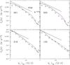 |
Fig. 6 The same as in Fig. 5, but for the shearing components of the velocity power spectra. |
| In the text | |
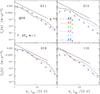 |
Fig. 7 The same as in Fig. 5, but the spectra here are computed for the quiescent testclusters. |
| In the text | |
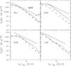 |
Fig. 8 As in Fig. 6, but for the quiescent test clusters. |
| In the text | |
|
Fig. 9 Shearing components of the density-weighted velocity power spectra are shown at z = 0 for the runs of the relaxed test clusters as a function of the wavenumber. As in the previous figures, different line styles are for different AV runs. In each panel runs with different resolution are displayed with different line thickness. For the sake of clarity, not all of the AV runs are plotted and runs with different AV parameters have been equispaced from top to bottom by a factor of 10. To more clearly illustrate the wavenumber dependence, spectra have been computed here using |
| In the text | |
|
Fig. 10 The ratio of the longitudinal to total velocity power spectra are shown at z = 0 for runs of the relaxed test clusters as a function of the wavenumber. The line coding is the same as in the previous figure; runs with different AV parameters have been equispaced from top to bottom by a factor 0.2. |
| In the text | |
|
Fig. 11 Transverse (S ∥ ) and longitudinal (S ⊥ ) second-order normalized velocity structure functions at z = 0 for HR runs of the perturbed test clusters as a function of r/r200. |
| In the text | |
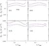 |
Fig. 12 As in Fig. 11, but for the density-weighted velocity structure functions. |
| In the text | |
|
Fig. 13 Final radial entropy profiles for the HR runs of the relaxed test clusters. Gas entropy is defined as |
| In the text | |
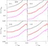 |
Fig. 14 As in Fig. 9, but for the entropy profiles. |
| In the text | |
|
Fig. 15 As in Fig. 9, final profiles of the viscosity parameter α are shown for the runs of the relaxed test clusters with different AV parameters and resolution. In each cluster panel the profiles have been plotted without any shifting between the various cases. |
| In the text | |
|
Fig. 16 Final energy density radial profiles constructed from the HR runs of the dynamically perturbed test clusters. Each panel shows: the profile of the thermal energy density Eth = 3kBT(r)ρg(r)/2μmp, the kinetic energy density profile Ekin = ρgu2/2 and the turbulent one |
| In the text | |
|
Fig. 17 Ratio of the turbulent to the total pressure, Ptu/Ptot ≡ Eturb/Etot, for the profiles of Fig. 16. Additionally, for the same test runs, are shown (thin lines) the ratios of the “velocity” pressure to the total one : |
| In the text | |
|
Fig. 18 As in Fig. 7, compressive components of the density-weighted velocity power spectra are shown at the present epoch for the cooling HR runs of the relaxed cluster subsample. |
| In the text | |
|
Fig. 19 As in Fig. 15, final profiles of the viscosity parameter α are shown for the cooling runs of the perturbed test clusters with different AV parameters and resolution. |
| In the text | |
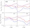 |
Fig. 20 As in Fig. 17, but for the cooling runs. |
| In the text | |
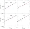 |
Fig. 21 As in Fig. 13, but for the cooling runs. |
| In the text | |
|
Fig. 22 Final radial profiles of the gas fraction fg(<r) = Mgas(<r)/Mcl(<r) are shown for the HR cooling runs of the perturbed cluster subsample in units of the cosmic value |
| In the text | |
Current usage metrics show cumulative count of Article Views (full-text article views including HTML views, PDF and ePub downloads, according to the available data) and Abstracts Views on Vision4Press platform.
Data correspond to usage on the plateform after 2015. The current usage metrics is available 48-96 hours after online publication and is updated daily on week days.
Initial download of the metrics may take a while.