| Issue |
A&A
Volume 525, January 2011
|
|
|---|---|---|
| Article Number | A37 | |
| Number of page(s) | 16 | |
| Section | Extragalactic astronomy | |
| DOI | https://doi.org/10.1051/0004-6361/201015520 | |
| Published online | 30 November 2010 | |
Spectral variability of quasars from multi-epoch photometric data in the Sloan Digital Sky Survey Stripe 82
1
Thüringer Landessternwarte Tautenburg,
Sternwarte 5, 07778
Tautenburg,
Germany
e-mail: This email address is being protected from spambots. You need JavaScript enabled to view it.
2
Astronomisches Institut, Universität Bern,
Sidlerstraße 5, 3012
Bern,
Switzerland
3
Astrophysikalisches Institut Potsdam, An der Sternwarte 16, 14482
Potsdam,
Germany
Received:
3
August
2010
Accepted:
27
September
2010
Abstract
Aims. The study of the ensemble properties of the UV/optical broadband variability of quasars is hampered by the combined effects of the dependence of variability on timescale, rest-frame wavelength, and luminosity. Here, we present a new approach to analysing the dependence of quasar variability on rest-frame wavelengths.
Methods. We exploited the spectral archive of the Sloan Digital Sky Survey (SDSS) to create a sample of over 9000 quasars in the Stripe 82. The quasar catalogue was matched with the Light Motion Curve Catalogue for SDSS Stripe 82 and first-order structure functions were computed from the lightcurves. The structure functions are used to create a variability indicator that is related to the same intrinsic timescales for all quasars (about 1 to 2 yr in the rest-frame). We study the variability ratios for adjacent SDSS filter bands as a function of redshift. A quantitative interpretation of these relations is provided by comparing with the results of simple Monte Carlo simulations of variable quasar spectra.
Results. We confirm the well-known dependence of variability on time-lag; the best power-law fit of the sample-averaged structure function has a slope β = 0.31 ± 0.03. We also confirm that anti-correlations exist with luminosity, wavelength, and redshift, where the latter can be fully explained as a consequence of the former two dependencies. The variability ratios as a function of redshift resemble the corresponding colour index-redshift relations. While variability is almost always stronger in the bluer passband than in the redder, the variability ratio depends on whether strong emission lines contribute to either one band or the other. We find that the observed variability ratio-redshift relations are described well assuming that (a) the r.m.s. fluctuation of the quasar continuum flux follows a power law σ(fλ) ∝ λ-2 (i.e., is bluer when brighter) and (b) the variability of the emission line flux is only ~10% of that of the underlying continuum. These results, based upon the photometry of more than 8000 quasars, confirm the previous findings by Wilhite and collaborators for 315 quasars with repeated SDSS spectroscopy. Finally, we find that quasars with unusual spectra and weak emission lines tend to have less variability than conventional quasars. This trend is the opposite of that expected from the dilution effect of variability due to line emission and may be indicative of high Eddington ratios in these unusual quasars.
Key words: galaxies: active / quasars: general / quasars: emission lines
© ESO, 2010
1. Introduction
The variation in flux density over time is one of the key characteristics of active galactic nuclei (AGN). From the onset of the study of quasars, which are the most luminous AGNs, variability is known to be a diagnostic property and has been successfully used as a criterion for selecting quasar candidates in a number of studies. On the other hand, the physical mechanisms behind these fluctuations are still poorly known, though it has long been understood that the observed flux variations of AGNs hold keys to the structure of the radiation source. The advent of modern variability surveys (e.g., Ivezić et al. 2003; Groot et al. 2003; Becker et al. 2004; Bauer et al. 2009; Djorgovski et al. 2008; LSST Science Collaborations 2009) combining high photometric accuracy, large survey areas, sufficiently long time baselines, and a high number of observation epochs holds the promise of significant progress.
Numerous studies have shown that the optical/UV continuum variability of quasars correlates with various physical parameters such as time-lag, rest-frame wavelength, luminosity, radio properties, emission line properties, and the Eddington ratio (e.g., Ulrich et al. 1997; Giveon 1999; Helfand 2001; Gaskell & Klimek 2003; Vanden Berk et al. 2004; Rengstorf et al. 2006; Wold et al. 2007; Wilhite et al. 2008; Bauer et al. 2009; Ai et al. 2010; MacLeod et al. 2010; Schmidt et al. 2010). Despite considerable progress in the description of quasar variability, there are still conflicting claims about these correlations and their physical interpretation is fraught with problems. The most frequently discussed models for the continuum variability of AGNs include instabilities in the accretion disk (e.g., Kawaguchi et al. 1998), multiple supernovae (or other Poissonian processes; e.g., Terlevich et al. 1992; Cid Fernandes et al. 1997), star-star collisions in the dense circumnuclear environment (Torricelli-Ciamponi et al. 2000), and microlensing by compact foreground objects (e.g., Chang & Refsdahl 1979; Hawkins 1993, 2010; Lewis & Irwin 1996, Zackrisson et al. 2003).
Much of the knowledge about quasar variability is based on the detailed investigation of large, statistically well-defined quasar samples. Even though each individual lightcurve is poorly sampled, a large number of quasars and the wide range of parameter values allow us to distinguish the dependences of variability on the various parameters. Hence, substantial improvement has been achieved by employing the quasar data base from the Sloan Digital Sky Survey (SDSS; York et al. 2000; Abazajan et al. 2009). Using a sample of 25 000 spectroscopically confirmed quasars from the SDSS, Vanden Berk et al. (2004) parametrized correlations between variability and time-lag, luminosity, redshift, and rest-frame wavelength upon a time-baseline of up to ~2 yr in the observer frame. A sample of more than 41 000 quasars was studied by de Vries et al. (2005). By combining the SDSS photometric data with the Palomar Observatory Sky Survey (POSS), these authors achieved a baseline of up to 50 yr in the observer frame, yet with a very sparse lightcurve sampling per quasar.
Wilhite et al. (2005) selected a set of 315 quasars with multi-epoch SDSS spectroscopy to analyse variability from spectrophotometry. In this way, the wavelength dependence of quasar variability could be studied at spectral resolution high enough to allow the analysis of variability not only in the continuum but also in the major emission lines. The results confirm that the continua are bluer when brighter and clearly show that variability is weak in the emission lines. They provide a natural explanation of the intrinsic Baldwin effect behaviour of individual AGNs (Kinney et al. 1990; Wilhite et al. 2006). Pereyra et al. (2006) demonstrated that the composite flux differences in the rest-frame wavelength range 1300–6000 Å can be fit by a standard thermal accretion disk model in which the accretion rate has changed from epoch to epoch. These results suggest that the dominant fraction of the optical/UV variability of quasars is related to the accretion process. On the other hand, chromatic variability may also be produced by quasar microlensing as the continuum source is compact and bluer at smaller radii (Wambsganss & Paczyński 1991; Yonehara et al. 2008, and references therein). Wilhite et al. (2005) argued that the low variability of the broad emission lines provides a problem for the microlensing scenario as one would expect a higher fraction of events where the lense crosses the broad line region (BLR) but not the compact source. The BLR was once considered too large to be affected significantly by microlensing. Studies have shown, however, that the BLR can be small enough to be amplified significantly by stellar-mass objects (Abajas et al. 2007, and references therein).
A 300 square degree area in the southern Galactic cap has been repeatedly imaged by the SDSS since 1998 and by the SDSS-II Supernova Survey (Frieman et al. 2008) since 2005. The multi-epoch observations in this SDSS Stripe 82 (S82) provide a useful database for the statistical analysis of quasar variability. Sesar et al. (2007) were the first to analyse the variable sources in S82 with the emphasis of characterizing the faint variable sky and quantifying the variable population as a whole. They present methods to select variable sources and discuss their distribution in the magnitude-colour-variability space. The three dominant classes of variables found by Sesar et al. are quasars (63%), RR Lyrae stars (7%), and stars from the main stellar locus (25%). Moreover, they demonstrate that at least 90% of the quasars are significantly variable. An interesting detail of this paper is a plot (their Fig. 7) of the ratio, Vg/Vr, of the variability V of quasars in the g- and r-band as a function of redshift z. Sesar et al. observe a feature in this diagram at z ~ 1.0–1.6 and argue qualitatively that it is due different parts of the spectrum varying in different ways. This is an important observation that offers a new possibility of investigating the spectral variability of quasars, which is obviously worth studying in detail.
The present paper is focussed on the variability ratios Qk,l = Vk/Vl as a function of redshift. The main aim is to derive the dependence of the variability on the (intrinsic) wavelength. In view of the combined effects of the dependence of the variability on wavelength, time, and luminosity, the ratios of the variabilities in different photometric bands provide a better approach to the spectral behaviour of variability than variability measured in a single band, as was pointed out by Sesar et al. (2007). The main differences from Sesar et al. are the following: (i) Sesar et al. used photometric measurements from 58 imaging runs from 1998 September to 2004 December. In the present study, the lightcurves are taken from the Light and Motion Curve Catalogue (LMCC) of the SDSS S82 (Bramich et al. 2008). The catalogue is based on 134 imaging runs obtained from 1998 to 2005 November with 62 runs obtained in 2005 alone. (ii) We extend the approach to all five SDSS bands. (iii) We use variability indicators related to (more or less) the same quasar-intrinsic timescale to eliminate z-dependent selection effects due to cosmological time dilation. (iv) Since the approach works only if quasar variability is dominated by the same processes at low and high redshift, we check whether this assumption is consistent with our data. (v) Finally, a quantitative interpretation of the diagrams is presented by means of numerical simulations. Compared to the spectroscopic sample of Wilhite et al. (2005), the quasar sample of the present study is much larger and the time baseline covered by the data is longer.
The creation of the quasar sample is described in Sect. 2. Variability indicators are computed from their lightcurves in Sect. 3. The resulting Qk,l-z relations for the five SDSS bands (k,l = 1...5) are presented in Sect. 4 and compared to the results of a simple parametrized model in Sect. 5. Other subjects in Sect. 5 are the comparison of our results with Wilhite et al. (2005) followed by a brief discussion of the variability properties of unusual quasars and the subsample of radio-loud quasars. Finally, Sect. 6 presents our conclusions. Standard cosmological parameters H0 = 71 km s-1 Mpc-1,Ωm = 0.27,ΩΛ = 0.73 are used throughout the paper.
2. The quasar sample
The SDSS seventh data release (DR7; Abazajan et al. 2009), marking the completion of the original goals of the SDSS and the end of the phase known as SDSS-II, contains over 1.6 million spectra in total, including 120 000 quasars. The quasar sample for the present study was constructed from the SDSS DR7 public archive of spectra in the region of the Stripe 82, i.e., right ascension α = 20h...4h and declination δ = −1°25... +1°25.
Whether a spectrum is useful for scientific purposes or not is indicated by the SciencePrimary flag, which is set to be either 1 or 0. Since SciencePrimary = 1 does not necessarily guarantee the correctness and precision of the cataloged quantities, we decided to download all spectra classified as quasars (Spec_cln = 3), regardless of their SciencePrimary flag, including all spectra classified as unknown (Spec_cln = 0). This last decision was motivated (i) by our aim of creating a quasar sample as large and complete as possible and (ii) the claim that interesting cases of rare unusual quasar spectra (e.g., Hall et al. 2002) might be hidden there. The list contains 20 542 objects of which 19 660 were available for download (13 224 with Spec_cln = 3 and 6436 with Spec_cln = 0). The quasar selection does not include AGNs classified spectroscopically as galaxies (Spec_cln = 2). We expect the majority of them to be low-redshift, low-luminosity AGNs, while the present study aims to compare the variability at different redshifts z = 0.2...3 and is restricted, therefore, to high-luminosity AGNs (Mi < −21, Sect. 4.3). Moreover, the stellar light from the host galaxies of low-luminosity AGNs tends to “dilute” the variability of the AGN.
All spectra were checked individually to estimate redshifts z and object types. Redshift values were computed automatically by comparing of measured line centres of the prominent emission lines with a catalogue of their rest-frame wavelengths. The spectral lines useful for the redshift (z) estimation were selected manually: this allows us to recognize and exclude quasar lines influenced by e.g., the remnants of bright night sky lines as well as Lyα lines affected by strong absorption of the blue wing. Dubious cases were flagged (Flag_z = 1). While the approach was not optimized to provide the highest accuracy z values, roughly erroneous redshift estimations could be efficiently suppressed, which is more important for the present study. The spectra were classified into the six types: quasar (q), possible quasar (q?), galaxy (g), star (s), unclear (u), and noise (n). For quasar spectra, special features such as strong broad absorption lines (BALs), unusual BALs, weak emission lines, or strong iron emission were noted. The procedure was performed twice for all 19 660 spectra.
Number of quasars from the basic catalogue with redshift deviations |zhere − zSDSS| > |Δz| max.
We assigned 13 558 selected spectra to the types q, q?, or g. To distinguish galaxies from quasars, a simple criterion was used where priority was given to low contamination by non-AGNs: spectra containing typical absorption lines and/or narrow emission lines but no signs of broad emission-line components were classified simply as galaxies. The total number of quasar spectra (type q) is 12 966, among them 976 from the database of the unknowns (Spec_cln = 0), another 4 objects were classified as possible quasars. Fiber positions that differ by less than the fibre diameter (3 arcsec) can be ascribed with high probability to the same object. After excluding multiple observations, the resulting basic catalogue contains 9855 entries with 2021 objects having been observed at least two times (660 objects with more than 2 spectra). For all objects with multi-epoch spectra, the z and type of the single spectra were compared with each other. Inconsistent results were found in only very few cases (e.g., because of corrupted spectra or low signal-to-noise ratio (S/N)).
We identified 8212 entries in our basic quasar catalogue with entries in the SDSS DR5 quasar catalogue (QC DR5; Schneider et al. 2007), 736 (7%) were found in the database of the unknowns only. Table 1 compares our redshift estimates with the z values from Schneider et al. (2007) and the DR7, respectively, for objects not listed in the QC DR5. The 25 quasars with dubious redshift flags from the present study were eliminated. While the agreement with the QC DR5 is satisfactory, we find that a substantial number of erroneous redshifts have been produced by the SDSS DR7 pipeline, which are attributed to erroneous line identifications (e.g., Mg II with Lyα, C IV, or C III]) in most cases.
To analyse variability, the basic quasar catalogue was matched to the LMCC (Bramich et al.
2008) using an identification radius of 2 arcsec.
The LMCC was trimmed to only those objects that have a mean right ascension in the range
α = 20.7h...3.3h because of the
sparse temporal coverage outside these limits. Compared to the whole S82, the area of sky
covered by the LMCC is thus reduced by ~17% to ~249 deg2. The final
quasar catalog contains 8 744 objects identified in the LMCC (Fig. 1). The redshifts cover the range
z ≈ 0.1...5 with  . Absolute magnitudes
Mi were computed following Kennefick and Bursick (2008; their equations 1 to 6) correcting the SDSS i band
magnitude for Galactic extinction and applying a standard continuum K
correction by assuming a spectral index
αν = −0.5. The Galactic foreground extinction
was obtained from the “Galactic Dust Extinction Service”1 of the NASA/IPAC Infrared Science Archive using the translation relations for
the SDSS bands given by Schlegel et al. (1998). The
mean value of the absolute magnitudes in the sample is
Mi = −24.7 ± 1.57. The distribution of the quasars in the
z-Mi plane is shown in Fig. 1.
. Absolute magnitudes
Mi were computed following Kennefick and Bursick (2008; their equations 1 to 6) correcting the SDSS i band
magnitude for Galactic extinction and applying a standard continuum K
correction by assuming a spectral index
αν = −0.5. The Galactic foreground extinction
was obtained from the “Galactic Dust Extinction Service”1 of the NASA/IPAC Infrared Science Archive using the translation relations for
the SDSS bands given by Schlegel et al. (1998). The
mean value of the absolute magnitudes in the sample is
Mi = −24.7 ± 1.57. The distribution of the quasars in the
z-Mi plane is shown in Fig. 1.
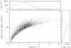 |
Fig. 1 Left: redshift versus absolute i band magnitude and histograms for the distributions of redshifts (top) and absolute magnitudes (right) for the final quasar sample. |
First five rows of the table containing the variability indicators Vk. The full table is available at the CDS.
To model spectral variability (Sect. 5.1), we needed to produce an average quasar spectrum. We used our “standard sample” (see Sect. 3.1 below) and constructed a composite following Vanden Berk et al. (2001). As we are primarily interested in “normal” quasars, objects with highly unusual spectra (remark = “x_bal” or “myst” in Table 2) are not included as well as quasars with uncertain redshifts. We also note that the sample is corrected for multiple observations; quasars with two or more SDSS spectra are thus represented by only one spectrum, usually the one with the highest S/N. All spectra were resized to a common range of 3900–9100 Å in the observer frame, sorted by increasing redshift, corrected for Galactic extinction, shifted into their rest-frame, and binned to a resolution of 1 Å per pixel. Subsequently each spectrum was inserted as a new row into a two-dimensional image, with 1 Å binning on the horizontal axis and one spectrum per pixel on the vertical axis. Every time before a new spectrum was inserted, a preliminary mean quasar spectrum was created simply by computing the mean pixel value for each wavelength bin in the two-dimensional image. The result is used for the normalisation: before inserting into the two-dimensional image, each spectrum is normalised to the mean pixel value of the overlapping region with the respective preliminary composite spectrum. The spectra was not assigned any statistical weights, i.e. the S/N of the spectra is assumed to be relatively constant throughout the sample and over the observed window. Pixels flagged “bad” in the SDSS 2D spectroscopic pipeline are interpolated over, and outliers and negative fluxes were excluded.
Composite spectra can be created in different ways. Vanden Berk et al. (2001) discussed how arithmetic and geometric mean composites have different properties. Following the arguments given by Wilhite et al. (2005), we consider the arithmetic composite but we prefer to use the median instead of the mean. The final composite spectrum is constructed by computing the median value for all wavelength bins represented by at least three spectra. The result is shown in the top panel of Fig. 2.
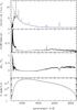 |
Fig. 2 Top: median composite spectrum from the final quasar sample with fitting power-law continuum. Second row: the semi-interquartile range, SIQR, in units of the median. Third row: relative deviation from the Vanden Berk et al. (2001) composite ([here-Vanden Berk]/here). Bottom: number of spectra per wavelength bin used for the construction of the composite. |
Vanden Berk et al. (2001) suggested using the semi-interquartile range, SIQR = (q3 − q1)/2 as a measure of the spectrum-to-spectrum variation, where q1 and q3 are the first (25%) and third (75%) interquartile; the second interquartile, q2, is the median. This ratio, SIQR/q2, is shown in the second panel of Fig. 2. There exist many spectra with a relative flux much higher or lower than the median at wavelengths where SIQR/q2 is high. On the other hand, if SIQR/q2 is small, the distribution is sharply peaked. As expected, the variation is huge in the wavelength range of the Lyα forest. At longer wavelengths, the variations are strong in the peaks of the emission lines, in particular of the [O iii] lines. Longward of ~4000 Å the spectrum-to-spectrum variation increases because of the different strong contribution of the host galaxies.
The third panel of Fig. 2 compares our median composite with that of Vanden Berk et al. (2001) where both spectra have been normalized normalized at 4000 Å. For wavelengths λ ~ 1000...4000 Å, our result (Fig. 2) is in accord with the Vanden Berk composite. The deviation at longer wavelengths reflects the differences in the quasar selection for the two samples. Vanden Berk et al. define “quasar to mean any extragalactic object with at least one broad emission line and that is dominated by a nonstellar continuum”. Spectra with continua dominated by stellar features were rejected by these authors “to avoid introducing a significant spectral component from the host galaxies”. This criterion was not applied in the present study. The consequence is a stronger contribution from host galaxies in our spectrum, yet the absolute magnitude-redshift plot appears to have a similar representation from low-luminosity AGNs in both cases. At short wavelengths, the differences are likely statistical fluctuations due to the small number of spectra included (bottom panel) in combination with the strong spectrum-to-spectrum variations at these wavelengths. In the spectral region between Ly α and 4000 Å, the continuum is matched by a power law fλ ∝ λαλ with αλ = −1.52 (αν = −0.48, in good agreement with αν = −0.46 given by Vanden Berk et al. for their arithmetic median composite).
The quasar catalog was matched to the FIRST (Becker et al. 1995) VLA 20 cm catalogue (match radius 2 arcsec). For the 467 identified FIRST sources, the values for the integrated 20 cm flux and the peak flux were entered. A radio compactness parameter and the radio loudness parameter Ri = log (Fradio/Fi) were computed following Ivezić et al. (2002); 381 sources are radio-loud (Ri > 1). Finally, more than 50 quasars were marked as having more or less unusual spectra, i.e., spectra that deviate remarkably from the typical quasar spectrum. The classification was performed by eye and is thus not based on quantifiable properties. The spectra of these objects display various unusual features that are difficult to discern at first glance, often (but not exclusively) related to complex broad absorption line (BAL) troughs combined with strong reddening (e.g., Hall et al. 2002). This subsample is inhomogeneous and includes unusual BAL quasars as well as weak emission line quasars (WLQs) and “mysterious” objects such as SDSS J010549.75-003314.0 and SDSS J220445.26+003142.0 from Hall et al. (2002). In several cases, the redshifts are uncertain. For one of these objects, SDSS J014349.14+002128.4, the spectrum was first classified as an unusual BAL quasar but later rejected after we found it to be a superimposition of the spectra of a normal quasar in the blue and an M star in the red.
3. Measuring spectral variability
3.1. Photometric data
The catalogue of objects in S82 compiled by Bramich et al. (2008) contains about 3.7 million stellar objects and galaxies. It comes in two flavours, the Light-Motion Curve Catalogue (LMCC), which contains the measured quantities for each object listed as a function of filter band and epoch, and the Higher-Level Catalogue (HLC), which contains similar quantities for each light-motion curve. Since the present paper intends to analyze the lightcurves, the LMCC is used here. For the overwhelming majority (≳90 %) of the quasars, the number of measurement epochs is between 20 and 50 with a mean at ~35 in all five bands. For a detailed description of the LMCC, we refer to Bramich et al. (2008) and address only three issues: (i) for an object record to be included in the LMCC, a list of constraints need to be satisfied in at least one waveband. In addition, we accept here only measurements, in each band, with the quality flags BRIGHT = 0, EDGE = 0, BLENDED = 0, and SATUR = 0. (ii) As noted by Bramich et al., the catalogue is contaminated by some strong photometric outliers that are clearly due to “bad epochs”. We find that some lightcurves show one, sometimes two, rarely more, examples of such low quality data that can significantly affect the measurement of variability. We applied a 2.5σ100-clip criterion to identify and eliminate the corresponding data points, where σ100 is the standard deviation of magnitudes in a 100 d time interval centred on the corresponding epoch. Each lightcurve was checked for up to three of these outliers. (iii) We restrict the analysis, in each band, to objects brighter than the limiting magnitudes 21.9, 23.2, 22.8, 22.2, and 20.7 for u, g, r, i, and z. More precisely, only quasars with mean magnitudes 0.5 mag brighter than the corresponding limit in each band were considered to minimize a possible bias by a one-sided censorship of the lightcurves due to variability.
As a first step, we estimate the fraction of significantly variable quasars. We use the
 per degree of freedom defined by Sesar
et al. (2007) to compare the magnitude fluctuations
of the quasars from the final sample with those of 1100 objects selected from the SDSS
standard star catalogue for S82 (Iveciź et al. 2007). The constraint
per degree of freedom defined by Sesar
et al. (2007) to compare the magnitude fluctuations
of the quasars from the final sample with those of 1100 objects selected from the SDSS
standard star catalogue for S82 (Iveciź et al. 2007). The constraint  (significance level
α = 0.05) is a useful criterion for significant quasar variability, i.e.,
the fluctuations cannot be explained by Gaussian-distributed measurement errors with the
same (magnitude-dependent) standard deviations as measured for the standard stars. Using
this criterion, we find that 93%, 97%, 93%, 87%, and 37% of the quasars are variable in
the u, g, r, i, and z band, respectively.
(significance level
α = 0.05) is a useful criterion for significant quasar variability, i.e.,
the fluctuations cannot be explained by Gaussian-distributed measurement errors with the
same (magnitude-dependent) standard deviations as measured for the standard stars. Using
this criterion, we find that 93%, 97%, 93%, 87%, and 37% of the quasars are variable in
the u, g, r, i, and z band, respectively.
We next consider whether variability is characterized more accurately by a normal
distribution of fluxes or magnitudes. Fig. 3 shows
the distribution of the normalized fluctuations 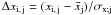 for the g-band measurements i of the significantly variable quasars
j, where x represents either magnitudes (left hand
side) or fluxes (right hand side) after the exclusion of outliers. The data are obviously
more accurately matched in the left panel, yet the agreement is not perfect. A lognormal
distribution of fluxes, i.e., a normal distribution of magnitudes, has been found for both
the optical and X-ray radiation of AGNs (Gaskell & Klimek 2003, and references therein).
for the g-band measurements i of the significantly variable quasars
j, where x represents either magnitudes (left hand
side) or fluxes (right hand side) after the exclusion of outliers. The data are obviously
more accurately matched in the left panel, yet the agreement is not perfect. A lognormal
distribution of fluxes, i.e., a normal distribution of magnitudes, has been found for both
the optical and X-ray radiation of AGNs (Gaskell & Klimek 2003, and references therein).
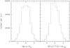 |
Fig. 3 Distribution of the normalized fluctuations of g-band magnitudes (left) and fluxes (right), respectively. Dotted curves: normalized, centred Gaussian distribution. |
As we are interested in the variability properties of typical, “normal” quasars, the unusual BAL quasars and the quasars with uncertain redshifts were removed from the sample. We also rejected the core-dominated radio-loud quasars. Vanden Berk et al. (2004) and Rengstorf et al. (2006) found the median integrated radio-flux density to be higher for the variable population of their samples than for the nonvariable population and suggested blazars as a possible explanation. The continuum emission mechanism for blazars differs fundamentally from that of other quasars (e.g., Ulrich et al. 1997). It is unlikely that all rejected radio-loud quasars belong to the blazar family but there might be a substantial fraction where both the flux and its variation are dominated by the relativistic ouT1low. In the following, we consider as our “standard sample” all quasars with known redshifts from the final sample without the unusual and the known radio-loud quasars. The latter two subsamples are discussed separately in Sect. 5.4.
3.2. Structure functions
The statistical measure of quasar variability used in the present paper is based on the first-order structure function (SF) D(τ), where τ is the time-lag between two observations. The SF is closely related to the autocorrelation function and contains, as a sort of running variance (as a function of the time-lag), information about the timescales of the involved variability processes. The SF was first introduced to quasar research in radio astronomy (Simonetti et al. 1985; Hjellming & Narayan 1986; Hughes et al. 1992) and has also become a popular tool in optical studies of both quasar samples and individual quasar lightcurves (e.g., Giallongo et al. 1991; Hook et al. 1994; Meusinger et al. 1994; Kawaguchi et al. 1998; Vanden Berk 2004; De Vries et al. 2005; Wilhite et al. 2008; Bauer et al. 2009; Schmidt et al. 2010). Scholz et al. (1997) were the first to use an index for long-term variability based on the observed SF to identify quasar candidates in an variability-based quasar survey (see also Meusinger et al. 2002).
There are three different definitions of the SF used in the literature. Here, we follow
the version introduced in the pioneering papers of Simonetti et al. (1985) and Hjellming & Narajan (1986), where the first-order SF is defined as ![Mathematical equation: \begin{equation} D(\tau) = \left\langle \left[s(t+\tau)-s(t)\right]^2 \right\rangle_{\rm t}, \label{eqn:SF} \end{equation}](/articles/aa/full_html/2011/01/aa15520-10/aa15520-10-eq81.png) (1)where s(t)
is the measured signal at time t, and the angular brackets denote the
time-average. The SF analysis in the optical/UV usually identify signals with apparent
magnitudes, i.e.,
s(t) = m(t). In a
second approach (e.g., Di Clemente et al. 1996;
Vanden Berk et al. 2004; Wilhite et al. 2008), ⟨[Δm] 2⟩ is
replaced by π/2 ⟨| Δm |⟩ 2. The former
was referred to as SF(A) and the latter as SF(B) by Bauer et al.
(2009). In a third version, here called
SF(C), ⟨| Δm |⟩ was used instead of
⟨[Δm] 2⟩ where ⟨ ⟩ means either the median (Hook
et al. 1994) or the mean (Schmidt et al. 2010). SF(A) has the advantage of being
directly related to other statistical quantities such as the variance and the
autocorrelation function, while SF(B) and SF(C) are less sensitive
to the presence of outliers in the data. Since we rejected the outliers in the process of
constructing the lightcurves (Sect. 3.1), we decided
to apply the “classical” definition from Eq. (1).
(1)where s(t)
is the measured signal at time t, and the angular brackets denote the
time-average. The SF analysis in the optical/UV usually identify signals with apparent
magnitudes, i.e.,
s(t) = m(t). In a
second approach (e.g., Di Clemente et al. 1996;
Vanden Berk et al. 2004; Wilhite et al. 2008), ⟨[Δm] 2⟩ is
replaced by π/2 ⟨| Δm |⟩ 2. The former
was referred to as SF(A) and the latter as SF(B) by Bauer et al.
(2009). In a third version, here called
SF(C), ⟨| Δm |⟩ was used instead of
⟨[Δm] 2⟩ where ⟨ ⟩ means either the median (Hook
et al. 1994) or the mean (Schmidt et al. 2010). SF(A) has the advantage of being
directly related to other statistical quantities such as the variance and the
autocorrelation function, while SF(B) and SF(C) are less sensitive
to the presence of outliers in the data. Since we rejected the outliers in the process of
constructing the lightcurves (Sect. 3.1), we decided
to apply the “classical” definition from Eq. (1).
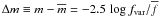
The general definition and some properties of the SF are given by Simonetti et al. (1985), an “ideal” SF of a “typical” measured process is schematically discussed by Hughes et al. (1992). For lags shorter than the smallest correlation timescale, T0, of the variable process, the SF is given by D0 ≡ D(τ ≪ T0) = 2ξ2, where ξ2 is the variance of the measurement noise. The SF corrected for the measurement noise is given by Dcorr(τ) = D(τ) − 2ξ2. For τ ≫ T1, the SF displays another plateau with D(τ) = 2σ2, where T1 is the longest correlation timescale and σ2 > ξ2 is the variance of the process. For the intermediate part, T0 ≲ τ ≲ T1, the SF of a stationary random process is characterized by a power law D(τ) ∝ τx, where the exponent depends on the power spectrum of the process.
We briefly note two other fundamental properties of the SF. First, the method is suited to the analysis of sparsely sampled lightcurves of non-periodic and non-sinusoidal processes. Second, provided that variability is quasar-intrinsic, the data obtained at the same epochs for quasars at different z cover different source-intrinsic timescales because of the cosmological time-dilation and are thus not directly comparable. This problem can be avoided using the SF as a function of the rest-frame time-lag τr = τo/(1 + z). Giallongo et al. (1991) were the first to introduce an indicator for optical quasar variability based on the rest-frame SF.
In the following, variability is measured by the first-order structure function,
corrected for measurement errors and binned into rest-frame time-lag intervals
 (2)where
  is the variance in the measurement noise
for starlike objects of the apparent magnitude
is the variance in the measurement noise
for starlike objects of the apparent magnitude  adopted from the standard stars, where
 is the mean magnitude of the quasar. The
angular brackets denote the arithmetic mean over a suitable interval of rest-frame
time-lags around τr.
is the mean magnitude of the quasar. The
angular brackets denote the arithmetic mean over a suitable interval of rest-frame
time-lags around τr.
3.3. Spectral variability
For the investigation of the wavelength dependence, the variability is measured by one single value Vk for each quasar in each of the five SDSS bands k = 1...5. Distinguishing the V(λ,L,z) relations requires two steps. As suggested by Sesar et al. (2007), we consider the ratio Qk,l ≡ Vk/Vl of the variabilities in two adjacent photometric bands (k = 1...4,l = 2...5) instead of Vk itself. Second, to eliminate z-dependent selection effects due to cosmological time dilation, the τr interval has to be chosen properly. The latter is constrained by the following criteria:
-
Equation (1) yields discrete data points for eachquasar in the D-τ diagram. The mean SF ⟨D(τr)⟩ τr is computed by averaging these data within discrete τr bins. The binning intervals must be wide enough to cover a large number of data points.
-
D(τr) must be related to the same τr interval for all quasars independent of z.
-
Because quasar variability increases monotonically with τr up to timescales of ~40 yr (deVries et al. 2005), τr should be as long as possible.
-
The maximum rest-frame time-lag is τr,max ~ 7 yr (for z ~ 0), set by the time baseline of the LMCC.
-
To investigate the wavelength dependence, variability has to be measured in narrow z bins (see below). The z distribution for our final quasar sample (Fig. 1) shows a strong decline at z ≳ 2. Beyond z ~ 3, the number of quasars per z bin becomes too small for a statistical analysis.
Taken together, we find that τr = 300–600 days is an appropriate binning interval. We computed ⟨D(τr)⟩ τr to be the arithmetic mean of all D(τr) in this τr interval. The value Vk(τr) from the SF binned in this way is considered a useful variability indicator. The present analysis is thus related to variability processes with typical timescales of the order of ~1...2 years (rest-frame). The median rest-frame time-lag of 430 d is a factor of 3.5 longer than for the spectroscopic sample of Wilhite et al. (2005). This is an important advantage of the present data because of the increase in variability with time-lag (Fig. 4).
The variability indicators Vk for the 8 744 quasars from our final sample are given in Table 2, available at the CDS. The table contains the following information. Column 1 is the runnung number, Cols. 2 and 3 list right ascension and declination (J 2000) taken from the fits headers of the SDSS spectra. Columns 4 and 5 give the redshift and the redshift flag (=1 for uncertain redshifts, 0 otherwise). The g band magnitude is given in Col. 6 and the absolute magnitude Mi is given in Col. 7. The following five columns contain the variabilities V for ugriz. For ⟨D(τ)⟩ < 2ξ2, the value of Vk was set to zero, because negative values of Vk are unphysical. The last column contains information on specific spectral features (w_l: weak-line quasar, s_bal: strong BAL structure, x_bal: extreme BAL structure, myst: mysterious spectrum).
4. Results
4.1. Variability as function of time-lag
The binned, “noiseless” first-order structure functions averaged over our standard sample of quasars with Mi < −22 for u, g, r, i, respectively, are shown in Fig. 4. Seven time-lag bins were chosen in such a way that we have, on the one hand, log τ0 intervals of comparable widths and, on the other, reasonably large numbers of measurements in each bin. The vertical bars indicate the shift due to the corrections for instrumental errors ,which are large on short time-lags. As is evident from Fig. 4, variability increases with time-lag and decreases with rest-frame wavelength. The detailed investigation of the dependence of variability on rest-frame wavelength is the subject of Sect. 4.3. Here we discuss the dependence on time-lag.
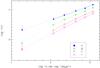 |
Fig. 4 Corrected ensemble-averaged structure functions for the quasars with Mi < −22 in the u, g, r, and i band as a function of time-lag. The time-lags are in the rest-frame, yet the SDSS bands are in the observer frame. |
In each of the four bands, the SF is closely fitted by a power law
![Mathematical equation: $[V(\tau_{\rm r})]^{1/2} \propto \tau_{\rm r}^{\ \beta}$](/articles/aa/full_html/2011/01/aa15520-10/aa15520-10-eq128.png) (following the notation of Kawaguchi
et al. 1998). No significant flattening of the SF
is observed at long time-lags. The slope of V(τ) in the
double-logarithmic presentation depends slightly on the chosen lag intervals and also on
the absolute magnitude threshold for the quasar sample. Results for the value of the
exponent β are listed in Table 3.
The uncertainties given there are the rms errors in the regression only. The total errors
are larger and are expected to be dominated by the uncertainties in the correction for
measurement errors, which may be underestimated here especially in the u band. (An
underestimation lowers the SF slope.) For Mi < −22, the
mean value of β, averaged over the high-throughput SDSS g,
r, and i filter bands, is β = 0.33 ± 0.01 for
τr > 10 days and 0.31 ± 0.03 for
τr > 100 days, respectively. The latter value is probably
more representative because the SF is less sensitive to the correction for measurement
errors at longer lags.
(following the notation of Kawaguchi
et al. 1998). No significant flattening of the SF
is observed at long time-lags. The slope of V(τ) in the
double-logarithmic presentation depends slightly on the chosen lag intervals and also on
the absolute magnitude threshold for the quasar sample. Results for the value of the
exponent β are listed in Table 3.
The uncertainties given there are the rms errors in the regression only. The total errors
are larger and are expected to be dominated by the uncertainties in the correction for
measurement errors, which may be underestimated here especially in the u band. (An
underestimation lowers the SF slope.) For Mi < −22, the
mean value of β, averaged over the high-throughput SDSS g,
r, and i filter bands, is β = 0.33 ± 0.01 for
τr > 10 days and 0.31 ± 0.03 for
τr > 100 days, respectively. The latter value is probably
more representative because the SF is less sensitive to the correction for measurement
errors at longer lags.
SF exponent β for different parameter selections.
SF exponent β from previous work and the present study.
A summary of SF slopes found in the literature is given in Table 4. The values for β scatter far more than expected from the individual errors. However, one has to take into account that the results are based not only on different quasar samples but also on different definitions of the SF (last column; see Sect. 3.2), different methods of averaging, different corrections of measurement errors, and different time baselines. Therefore, Table 4 also lists the definition and the maximum time-lag τmax (where “of” and “rf” refer to observer frame and rest-frame, respectively). The simple average of the previous results based on the SF(A), except for the Seyfert value from Hawkins (2002), yields 0.30 ± 0.07 (0.34 ± 0.11 for all data) which is close to the value from the present study. Frequently-quoted model predictions are β = 0.83 ± 0.08,0.44 ± 0.03, and 0.25 ± 0.03 for random superpositions of supernovae in the starburst model, instabilities in the accretion disk, and microlensing due to compact lenses in the foreground, respectively (Kawaguchi et al. 1998; Hawkins 2002). A tendency of the SF slope to increase with wavelength in the observer frame might be indicated in Table 3 (see also Schmidt et al. 2010; their Fig. 3).
The amplitudes of the SFs shown in Fig. 4 generally agree with findings in the literature listed in Table 4. De Vries et al. (2005; their Fig. 18) present a noise-corrected SF for combined g and r band as a function of time-lag in the observer frame. The last data point in our Fig. 4 corresponds to time-lags of ~7 yr where the de Vries SF predicts log V = −1.08, in perfect agreement with log V = −1.0 ± 0.1 for g and r in our study. De Vries et al. also show (their Fig. 9) that the time-lag shifted SF from Hawkins (2002) agrees with their data. The SF derived by Hook et al. (1994) corresponds to a lower amplitude of log V = −1.54 at τ ~ 7 yr (observer frame). The maximum lag of the data from Bauer et al. (2009) is ~103 d (rest-frame), but the amplitudes are not clearly defined at the longest time-lags. For log ⟨τr(d)⟩ = 2.5, Bauer et al. give log V = −1.6 without specifying the filter band, compared with −1.3 or −1.4 for g and r in the present paper. However, Bauer et al. emphasize that “the exact values for V should not be taken seriously ...because the data are arbitrarily normalized”. From the SFs presented by Wilhite et al. (2008; see also Rengstorf 2006) we derive log V = (−0.99, −1.17, −1.36, −1.44) for (u, g, r, i) at their maximum time-lags log ⟨τr(d)⟩ = 2.7, in good agreement with the values (−1.0, −1.15, −1.28, −1.35) found here for the same τr. The variability amplitudes derived from the SFs shown by Vanden Berk et al. (2004) are almost the same as in Wilhite et al. (2008). Kawaguchi et al. (1998) discuss the SF of only one quasar, hence their derived variability amplitude is not necessarily representative. We emphasize that these results are derived from SFs defined in different ways and computed from different quasar samples, that cover different ranges of time-lags, and are related to different frames (rest or observer).
4.2. Variability as a function of luminosity and redshift
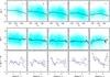 |
Fig. 5 Variability-absolute magnitude relations (top) and variability-redshift relations (middle) for the five SDSS bands. The bottom line compares the measured z gradient of variability (solid) with the z gradient expected from the dependence of V on Mi(z) (dashed). (Note that the Mi are K-corrected in the rest-frame, yet the Vk refer to photometric bands defined in the observer frame.) |
The sample-averaged variability measured in a given photometric passband is expected to
change with redshift because of the dependence of variability on absolute magnitude and
intrinsic wavelength. In addition, there might be an explicit dependence of variability on
redshift, i.e.,
V = V [Mi(z),λ(z);z]
and 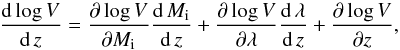 (3)where λ is the rest-frame
wavelength.
(3)where λ is the rest-frame
wavelength.
Figure 5 shows the distribution of the variable quasars (χ2 > 3) in the log V-Mi diagrams (top) and the log V-z diagrams (middle), respectively, for the five bands. We overplot the values of log ⟨V⟩ , where ⟨ ⟩ denotes the median within bins of the width 0.5 mag for Mi and 0.05 for z, respectively. For luminous quasars (here: Mi ≲ −25), the average variability decreases with luminosity. The relatively small variability of low-luminosity AGNs in the z band is expected because of the contribution of the host galaxy. The correlation with redshift is less pronounced but a slight tendency for larger variability at lower redshifts is apparent for the u and g band.
The solid polygon curves in the bottom row of Fig. 5 are the gradients dlog V/dz (i.e., the left-hand side of Eq. (3)) derived from the median relations shown in the middle row. The dashed lines represent the fraction corresponding to the Mi-z relation (i.e., the first term on the right-hand side of Eq. (3)) computed from the log ⟨V⟩ -Mi relation from the top line and the ⟨Mi⟩ -z relation from Fig. 1. In principle, the difference between the two curves can be used to derive the wavelength dependence of variability provided that there is no significant explicit redshift dependence of the variability. In particular, that the solid curves have generally higher values than the dashed curves at higher z indicates that V increase towards lower intrinsic wavelengths. However, the V-λ relation derived in that way is much too noisy to provide useful information. The observed V-z relation is dominated by the V-Mi(z) relation as indicated by the similarity of the two curves. A more effective approach to the V-λ relation will be discussed in Sect. 4.3 below.
To search for an explicit z dependence, we compare the variability
measured at different z but the same intrinsic wavelengths for quasars of
the same absolute magnitudes. This can be achieved with the present sample thanks to the
large number of quasars and the simultaneous measurements in five bands. We select the
variable quasars in the narrow absolute magnitude interval
Mi = −25 ± 0.5, where the coverage in the redshift space is
good for z ~ 0.5...2.2. For each rest-frame
wavelength λ ~ 1000...4000 Å, we computed the
redshift intervals
zk ± Δzk/2,
where λ is shifted into the u, g, r, and
i passbands, respectively, i.e.,
 and
Δzk = Δλk/λ
where
and
Δzk = Δλk/λ
where  is the mean wavelength and
Δλk the width of the corresponding band in
the observer frame (k = 1...4).
is the mean wavelength and
Δλk the width of the corresponding band in
the observer frame (k = 1...4).
The top panel of Fig. 6 shows the mean variability in the redshift intervals around zk(λ) as a function of intrinsic wavelength λ. At fixed λ, the band k corresponds to the redshift zk(λ). At wavelengths where there is an overlap of measurements in at least two bands, the comparison of the curves provides information on V(z). With a mean value of ⟨dV/dz⟩ = 0.001 ± 0.007 for 1000 Å < λ < 3500 Å, it is clearly seen (bottom panel) that there is no significant explicit variation in V with z for medium-luminosity quasars between z ~ 0.5...2. In addition, an increase in variability towards shorter wavelengths is clearly apparent in all bands (top panel). We note however that the absolute values of V(λ) are not representative for the whole sample because of the V-Mi relation.
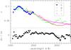 |
Fig. 6 Variability as a function of intrinsic wavelength (rest-frame) (top) and gradient d V/d z (bottom) for quasars with −24.5 > Mi > −25.5 (same scale for both parts of the diagram). |
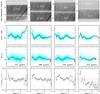 |
Fig. 7 Top: spectral coverage of the quasar composite spectrum by two adjacent photometric bands k,l (k = u,g,v,r and l = g,v,r,i,z) as a function of redshift z. The next rows (top to bottom) show the corresponding colour indices mk − ml, the variability ratios Qk,l, and the gradients dlog Qk,l/dMi, respectively. Polygons: medians of colour index and log Qk,l, respectively. |
4.3. Variability as a function of intrinsic wavelength
As outlined in Sect. 3.3, variability ratios Qk,l were computed for each quasar to measure how variability changes from band to band, thus with wavelength. The fundamental advantage is that the Qk,l are expected to be much less (or not at all) contaminated by a dependence of variability on luminosity (Sesar et al. 2007). The approach is based on the assumption that quasar variability is dominated by the same processes at high and low redshifts. We argue that this assumption is supported by our finding that there is no indication of an explicit dependence of variability on redshift in our sample. The variability ratios refer to the same intrinsic time-lags of 300 to 600 days for all redshifts.
In the following, we consider only AGNs with Mi < −21 and z = 0.2...3 because of the small number per bin outside this redshift interval. As in the previous subsections, we remove the relatively small fraction of unusual BAL quasars, core-dominated radio-loud quasars, and the few objects with uncertain redshifts. The final number of quasars is large enough to bin the data into small z intervals of width Δz = 0.05. In each of the 56 z bins, the sample-averaged ratio ⟨Qk,l(z)⟩ carries information about the variability at five different intrinsic wavelengths λk. The ensemble variability is thus measured at 56 × 5 = 280 different intrinsic wavelengths. Across the wavelength range λ ~ 800...8500 Å, the formal resolution of the intrinsic variability spectrum is therefore (8500−800) Å/280 ~ 28 Å. The spectral resolution can be improved by a factor ~2 by choosing narrower z bins.
The results are shown in the third row of Fig. 7. The dots are the Qk,l per quasar on a logarithmic scale with k and l referring to the SDSS bands (λk < λl) shown in the first row of the same column. The curves are the log ⟨Qk,l⟩ − z relations where ⟨ ⟩ denotes the median in z bins of the widths 0.05. Only quasars with significant variability (χ2 > 3; Sect. 3.1) in both the k band and the l band were included. The number of involved quasars is given in each panel. In the high-throughput bands, more than 7000 variable quasars are available. For most redshifts variability is, on average, stronger in the shorter wavelength bands than at longer wavelengths. But it is also obvious from Fig. 7 that the variability ratios display a complicated, nearly undulating dependence on z.
The z-dependence of the variability ratios can be qualitatively understood by comparing with the second row of Fig. 7 where the colour indices, mk − ml, are shown as a function of redshift. The variability ratios and the colour indices have a very similar dependence on redshift, though the scatter is clearly larger for the former. This similarity was first noted by Sesar et al. (2007) for the g and r band in the redshift interval 1.0...1.6 and is shown here to also exist for the other bands and across a broader z range. The structure in the colour index-redshift diagrams is known to be caused by the strong emission lines. To illustrate this effect, we show in the top row of Fig. 7 the quasar composite spectrum in the observer frame (vertical direction) as a function of z (horizontal direction). The spectrum has been multiplied with the transmission curves of the corresponding SDSS bands. The most prominent emission lines are labelled. The colour index Δmk,l decreases when a strong line enters the band k and increases at redshifts where the line leaves the band k and enters the band l. The effect is most clearly indicated by the Mg ii λ2800 Å line where there are no other strong lines around. The line dominates the u, g, r, i, z band at z ~ 0.3,0.7,1.2,1.7,2.2, respectively. u − g is consequently quite blue at z ~ 0.3 but redder at 0.7, g − r is blue at 0.7 but red at 1.2 etc.
The variability ratios vary with z in the opposite way to the flux ratios. When the flux ratio fk/fl increases because a strong line enters the band k, the variability ratio decreases. This can be explained only by the assumption that lines are significantly less variable than the continuum at the same wavelengths. Strong emission lines “dilute” the variability in the corresponding band. Hence, the ⟨Qk,l⟩ -z relation contains information on the wavelength dependence of the quasar variability and on the relative fraction of variability in the continuum and in the lines. In the next section, we use a simple parametrized model to quantify this relation. There is no hint of a correlation between the deviations of the flux ratios and the variability ratios from their median relations.
The bottom line of Fig. 7 shows that, at a given redshift, the variability ratio Qk,l also depends on luminosity. Interestingly, the gradient dlog Qk,l/dMi varies in a way with z that resembles the variation in the variability ratios itself.
5. Discussion
5.1. Numerical simulations
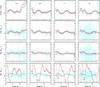 |
Fig. 8 Comparison of simulations (open symbols) and observations (thin curves and 1σ deviations): colour indices (top) and variability ratios as functions of redshift for the best-fit model with with small line variability (κ = 0.11; second row), the same model with large line variability (κ = 1; third row), and for a model where only the line flux is variable (bottom), respectively. |
To interpret the results from Fig. 7 quantitatively, we performed Monte Carlo simulations of variable quasar spectra. As a first step, the composite spectrum was decomposed into three components: the continuum fcont, the emission line portion flines, and the host galaxy contamination fhost2. We assumed that the continuum is the underlying variable source, the lines are much less variable, and the contribution of the host does not vary.
A simple method was used for the decomposition. The continuum fcont was described by the power law fitted to the composite between Ly α and 4000 Å, fcont ∝ λ-0.48 (Sect. 2). The power law was extrapolated down to 800 Å and a wavelength-dependent correction factor cH(λ) for the heavy Ly α forest absorption was derived shortward of Ly α. The product cHfcont was subtracted from the composite and the result shortward of 4000 Å was identified with the UV emission-line portion. The result longward of 4000 Å is the superimposition of the optical emission lines with the host spectrum. The host contribution was approximated by fitting by eye a smooth function to the stellar continuum. After parametrizing the variability as a function of wavelength, this rough decomposition enabled us to simulate variable spectra and analyse at least the general trends.
The variability was parametrized by assuming Gaussian-distributed magnitude fluctuations,
Δm, (see Sect. 3.1). The standard
deviation σΔm(λ) is
described by a power-law dependence on the intrinsic wavelength λ. Hence,
the variable portion of the spectrum was represented by
 where
where
 and
and
 was the variable portion of the composite
spectrum. The exponent was computed as
Δm = Δmnormσ(λ)
where Δmnorm is a random number for each single realization of
a variable spectrum. For n realizations of the same spectrum,
Δmnorm follows a centred and normalized Gaussian
distribution.
was the variable portion of the composite
spectrum. The exponent was computed as
Δm = Δmnormσ(λ)
where Δmnorm is a random number for each single realization of
a variable spectrum. For n realizations of the same spectrum,
Δmnorm follows a centred and normalized Gaussian
distribution.
The aim of the simulation was to compute the variability ratios
Qk,l as a function of redshift to
estimate the parameters of the power law as well as the line variability fraction
κ from the comparison of the simulated with the observed data. We adopt
 with
κ = 0...1. Hence, a realization of a quasar spectrum
is given by
f(λ) = fvar(λ) + (1 − κ)flines(λ) + fhost(λ).
The simulations cover the same redshift range as the observations. After transforming into
the observer frame, the “observed” spectrum is multiplied by the response functions of the
five SDSS filter bands and the total flux in each band is transformed into a magnitude.
From these data, colour indices and variability ratios are computed.
with
κ = 0...1. Hence, a realization of a quasar spectrum
is given by
f(λ) = fvar(λ) + (1 − κ)flines(λ) + fhost(λ).
The simulations cover the same redshift range as the observations. After transforming into
the observer frame, the “observed” spectrum is multiplied by the response functions of the
five SDSS filter bands and the total flux in each band is transformed into a magnitude.
From these data, colour indices and variability ratios are computed.
A parameter study was performed to find the best-fit model with 20 realizations of a
spectrum per redshift bin. The Mersenne Twister MT199373 random number generator was used, which passes various tests such as the
stringent "dieharder" test suite for randomness4. The
agreement between the simulated variability ratios Qsim and
the observed ratios Qobs is measured by the sum of the
(Qsim − ⟨Qobs⟩)2
over all redshift bins, where ⟨ ⟩ indicates the average in the redshift bin. We started
with the assumption that the variability in the lines is negligible
(κ = 0). The best fit is found for 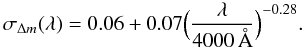 (4)The parameter κ was
subsequently varied; closest agreement was found for κ ~ 0.1.
(4)The parameter κ was
subsequently varied; closest agreement was found for κ ~ 0.1.
The simulated variability ratios of our best-fit model are shown in the second row of Fig. 8. The general agreement between the observed and the simulated relations is good. Most of the features seen in the mean observed relations are closely reproduced by the simulations. Exceptions are the low-redshift range for the redder bands and the high-redshift range for the bluer (z ≳ 2 for Qu,k and z ≳ 2.7 for Qg,r). The former is attributed to the rough modelling of the host contribution to the spectrum. The latter probably indicates an inconsistency of the composite spectrum at shortest wavelengths (λ ≲ 1100 Å) with the photometric data producing also a discrepancy for the colour indices. It is expected that a more elaborated method for the spectrum decomposition and an individual treatment of the strongest lines (Sect. 5.2.2) will provide an improved fit.
The third row of Fig. 8 shows the results from the same model with κ = 1. The comparison with model κ = 0.1 clearly indicates that most of the structure seen in the Qk,l-z relations is due to the small variability of the lines. In addition, the influence of the host galaxy is evident in the redder bands at low redshifts. For κ ≳ 0.2, the structure in the simulated curves is noticeably smeared increasingly with increasing κ. Finally, the structure reverses for models where only the line component is variable (bottom line of Fig. 8).
5.2. Comparison with Wilhite et al. (2005)
5.2.1. Colour variability
On the basis of the analysis of spectra of quasars with repeated SDSS spectroscopy, Wilhite et al. (2005) discuss the redshift dependence of colour differences Δ(mk − ml) = (mk − ml)bright − (mk − ml)faint. There is a change in colour that is a function of redshift and the filter used (their Fig. 14). As pointed out by those authors, the features in these diagrams are related to the relative lack of variability in the emission lines. In all colours, quasars appear bluer in the bright phase at almost all redshifts. This behaviour is modulated by, with changing redshift, strong emission lines being shifted in or out of the passbands. When a strong line shifted into the band k is less variable than the continuum, the fraction of the line flux to the continuum flux is larger in the faint phase than in the bright phase making (mk − ml)faint bluer than expected from the power-law continuum and the colour difference Δ(mk − ml) redder. The features in Fig. 14 of Wilhite et al. can be directly compared to those seen in the third line of our Fig. 7. For example, the first “red bump” in their Δ(u − g) versus z diagram at z ~ 0.35 corresponds to the minimum of Qu,g i.e., where the variability in u is low compared to g, and the “blue dip” at z ~ 0.75 corresponds to a maximum of Qu,g. In this way, all dips in the four colour-redshift diagrams in Fig. 14 of Wilhite et al. can be identified with bumps in the Qk,l diagrams in our Figs. 7 and 8.
5.2.2. Emission line variability
Wilhite et al. (2005) estimate the fraction of variability in the lines from 20% to 30% for C iv, C iii], and Mg ii. This result differs significantly from the 10% we find from fitting the variability ratios. For κ > 0.2, the structures in the simulated Qk,l-z relations are remarkably lower and the agreement with the observations becomes worse. However, our parameter κ is an integral quality that is averaged over all lines.
In this context, we note that even our best-fit model is not perfect. In particular, the slight systematic shift towards lower z of the structure related to the Mg ii line in the simulated curves is most likely due to differences in the variability fraction of Mg ii and the lines in the 3000 Å bump. More detailed simulations with an individual treatment of the strongest lines will certainly improve the fit and provide insight into the relative strengths of the variability of these lines.
5.2.3. Continuum variability
The standard deviation σ in the flux variation as a
function of wavelength is shown at the top of Fig. 9 for our best-fit model from Fig. 8. The
fluxes in the lines were assumed to vary by 10%, hence the lines are visible in this
diagram. For λ ≳ 2500 Å, the continuum variability is fitted by a power
law 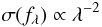 (5)in perfect agreement with the slope of the
geometric mean difference spectrum from Wilhite et al. (2005). This means in particular that the variability spectrum is steeper
(i.e., bluer) than the flux spectrum.
(5)in perfect agreement with the slope of the
geometric mean difference spectrum from Wilhite et al. (2005). This means in particular that the variability spectrum is steeper
(i.e., bluer) than the flux spectrum.
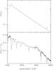 |
Fig. 9 Top: wavelength dependence of the standard deviation
σ of the flux density
fλ for the best-fit model with
κ = 0.1. The dashed line corresponds to the power law with
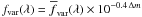
slope −2. Bottom: ratio |


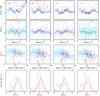 |
Fig. 10 Colour indices, mk − ml, (top) and variability ratios, Qk,l, (second row) as a function of redshift and variability index, Vk, as a function of absolute magnitude, Mi, (third row) for radio-loud quasars (dots) and quasars with unusual spectra (squares and arrows), respectively. Curves and hatched areas as in Fig. 8, filled squares in the third row: unusual quasars with weak emission lines (Fig. 11, left panel). Bottom: normalized distributions of log Vk for the unusual quasars (open squares and dashed lines), the radio-loud quasars (dots and dotted lines), and the standard sample (solid). |
Wilhite et al. (2005) found that the ratio of their arithmetic-mean composite difference-spectrum to the arithmetic-mean composite quasar-spectrum is almost one for λ ≳ 2500 Å and the ratio strongly increases towards shorter wavelengths at λ ≲ 2500 Å. The ratio of the standard deviation in our best-fit model to our arithmetic-mean composite is shown in the bottom panel of Fig. 9. We confirm that this ratio is approximately constant in the wavelength range between the the Mg ii line and λ ~ 4000 Å. However, there is a dip shortward of Mg ii in both our Fig. 9 (bottom) and the corresponding Fig. 13 of Wilhite et al., which leads to the impression of an abrupt increase shortward of ~2400 Å. In our model, this dip is attributed to the very broad conspicuous “contamination” feature from ~2300 to 4000 Å (see Vanden Berk et al. 2001). This so-called small blue bump (3000 Å bump) consists of a large number of weak Fe ii emission lines blend together to form a pseudo-continuum above the intrinsically emitted continuum, superimposed on the Balmer continuum emission (Wills et al. 1985; Vestergaard & Wilkes 2001). We argue therefore that the variability increases rather continuously towards short wavelengths for λ ≲ 4000 Å. At longer wavelengths, our ratio decreases dramatically, in contrast to that of Wilhite et al. However, this difference is expected since our sample is dominated by low-luminosity AGNs at low redshifts and the contribution from the host galaxies (λ ≳ 4000 Å) to our composite spectrum is thus much larger than in Wilhite et al.
5.3. Luminosity dependence of variability ratios
The behaviour of the luminosity dependence of the variability ratios as a function of
redshift (bottom row of Fig. 7) can be qualitatively
understood as follows. We assume that Fcont,k
and Fline,k are the total fluxes of the
continuum and the emission lines, respectively, in the band k. If the
lines are far less variable than the continuum, the fraction of the continuum flux
ρk = Fcont,k/(Fcont,k + Fline,k)
is a measure of the strength of variability at a given redshift. The variability ratio
Qk,l is then expected to scale with the
ratio
ρk/ρl.
For an average quasar spectrum and at given z, the luminosity scales with
the total flux
Ftot = Fcont + Fline
in a given band. Hence 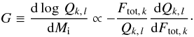 For simplicity, we consider the case where
there is only one strong emission line (e.g., Mg ii) in band k
for z ~ z1 and in band
l for
z ~ z2 > z1.
Hence
For simplicity, we consider the case where
there is only one strong emission line (e.g., Mg ii) in band k
for z ~ z1 and in band
l for
z ~ z2 > z1.
Hence 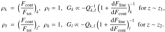 The gradient G depends
directly on the variability ratio and, in addition, on the relationship between the line
flux and the continuum flux in the band. The equivalent widths of the broad UV emission
lines is known for a long time (Baldwin 1977; Osmer
et al. 1994) to be inversely correlated to the
luminosity of the underlying continuum in a nonlinear way. This well-known Baldwin effect
appears in two flavours: (i) a global relationship that describes fluctuations from object
to object and (ii) an intrinsic relationship that describes how the line flux changes when
the continuum of the same object changes because of variability (Kinney et al. 1990; Pogge & Peterson 1992). In addition, however, the variation in G with
z also reflects the response functions of the SDSS bands because the
ratio of the line flux to the continuum flux in the band depends on the throughput at the
wavelength of the line. To summarize, the G-z relation
(bottom line of Fig. 7) reflects the
Qk,l-z relation, which is,
however, modified by both the Baldwin effect and the filter response curves.
The gradient G depends
directly on the variability ratio and, in addition, on the relationship between the line
flux and the continuum flux in the band. The equivalent widths of the broad UV emission
lines is known for a long time (Baldwin 1977; Osmer
et al. 1994) to be inversely correlated to the
luminosity of the underlying continuum in a nonlinear way. This well-known Baldwin effect
appears in two flavours: (i) a global relationship that describes fluctuations from object
to object and (ii) an intrinsic relationship that describes how the line flux changes when
the continuum of the same object changes because of variability (Kinney et al. 1990; Pogge & Peterson 1992). In addition, however, the variation in G with
z also reflects the response functions of the SDSS bands because the
ratio of the line flux to the continuum flux in the band depends on the throughput at the
wavelength of the line. To summarize, the G-z relation
(bottom line of Fig. 7) reflects the
Qk,l-z relation, which is,
however, modified by both the Baldwin effect and the filter response curves.
5.4. Special quasar types
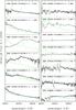 |
Fig. 11 Left: unusual quasar spectra with weak emission lines. Right: another 7 unusual quasars with weak variability (right). In each panel, the composite spectrum is overplotted as smooth curve (arbitrarily scaled). |
Among the 8744 objects in our final quasar sample, there are 54 quasars with unusual spectra and 454 quasars were identified with FIRST radio sources. Adopting the criterion Ri ≡ log (Fradio/Fi) > 1 (Sect. 2), we identified 381 radio-loud quasars in our sample. In Fig. 10, the optical colours and variability properties of both subsamples are compared with those of our standard quasar sample. As was noted by Richards et al. (2001) and Ivezić et al. (2002), the median colours are slightly redder and the fraction of red outliers is higher for the radio-loud subsample than for the standard sample, where the most extreme outliers are seen in the bluer passbands. A substantial fraction of the radio-loud subsample are also outliers in the Qk,l-z diagrams. In particular, there is more than a dozen quasars with low Qk,l, i.e., Vi > 2Vr.
For the subsample of quasars with unusual spectra, the deviation from the standard sample is much stronger. The colour indices u − g and g − r are much redder than for both the standard sample and the radio-loud subsample. These differences are again most pronounced for the bluer passbands and vanish for i − z. This result is not surprising. Both dust absorption and extended and/or overlapping BAL troughs in the UV, which are two defining features of this classification, have the effect of reddening especially the colour indices of the blue passbands. In this context, the scatter in the variability ratios might be expected to be explained by the diversity of the fraction of the emission-line flux in strong and unusual BAL quasars.
The fraction of radio detections among the unusual quasars is 17% (9/54) and the fraction of radio-loud quasars is 11% (6/54). The corresponding values for the whole sample are 5.2% (454/8744) and 4.4% (381/8744). This difference is, of course, due to SDSS having targeted FIRST sources for spectroscopy even when they were not selected as quasar candidates because of their optical colours. The three unusual quasars with the highest radio-loudness parameters are SDSS J000051.56+001202.5 (Ri = 1.89), a high-redshift (z = 3.859) BAL quasar with broad Lyα, Si iv, and C iv absorption troughs, SDSS J024224.02+010452.5 (Ri = 1.52), a medium-redshift (z = 2.431) quasar with apparently weak emission lines and associated absorption lines, and SDSS J022337.76+003230.6 (Ri = 1.77), a weak-line quasar at z ~ 3.05. The first two are strongly variable in the optical, whereas SDSS J022337.76+003230.6 exhibits a remarkably low level of variability in the u and g bands.
As a main result of Sects. 5.1 and 5.2, we have seen that the flux in the emission lines is considerably less variable than the underlying continuum. A relatively low variability Vg is thus expected at z ~ 3 where the strong Lyα+N v lines fall into the g band (see also Fig. 5). However, the value of Vu for SDSS J022337.76+003230.6 is a factor of 20 smaller than the mean value at z = 3 and, surprisingly, SDSS J022337.76+003230.6 is a member of the rare class of weak emission-line quasars (WLQs; Diamond-Stanic et al. 2009). WLQs are defined as quasars with extremely weak or undetectable emission lines of rest-frame equivalent width EW Å compared to ~50...100 Å for typical SDSS quasars (e.g., Fan et al. 1999; Diamond-Stanic et al. 2009, and references therein). For SDSS J022337.76+003230.6, Diamond-Stanic et al. measured EW Å. Quasars with such weak lines might be expected to exhibit larger variability in the passbands of the lines than typical quasars. This is clearly not the case for SDSS J022337.76+003230.6. Altogether the Diamond-Stanic WLQ sample contains four quasars in S82, three of them being members of our quasar sample where two have small variability (SDSS J022337.76+003230.6 and SDSS J005421.42-010921.6) and the third (SDSS J025646.56+003858.3) has values close to the medians.
If the weak lines are due to the Baldwin effect, WLQs might be expected to populate the high-luminosity end of the quasar luminosity function, which is obviously not the case (Shemmer et al. 2009, and references therein). The first interpretation of the nature of WLQs involved continuum boosting (Fan et al. 1999) as in local BL Lac objects. However, the rest-frame 0.1–5 μm spectral energy distributions of WLQs does not differ from those of normal quasars and variability, polarization, and radio properties differ from those of BL Lacs (Diamond-Stanic et al. 2009). In addition, Shemmer et al. (2009) pointed out that it would be difficult to explain the lack of a large parent population of X-ray and radio bright weak-lined sources at high z if WLQs were the long-sought high-redshift BL Lacs. Shemmer et al. (2006) argued against the possibility that WLQs are quasars with continua amplified by microlensing. This interpretation is also questioned by the low variability found in the present study based on intrinsic timescales of 1 to 2 yr, which are typical timescales for quasar microlensing.
Among the quasars classified here as unusual, no additional one matches the classical criterion of WLQs (i.e., EW Å). We note that our quasar sample is biased against spectra that have only a featureless continuum (Sect. 2). However, we selected (by eye) another five quasars for which the emission lines are substantially less pronounced than in the composite spectrum but where there is no clear-cut evidence of BAL troughs. Their spectra are shown in the left panel of Fig. 11 along with the WLQ SDSS J022337.76+003230.6. SDSS J220445.27+003141.8 (z = 1.353) is one of the two “mysterious objects” from Hall et al. (2002). The interpretation of SDSS J010605.07-001328.9 is unclear but the spectrum resembles the unusual FeLoBAL quasar VPMS J134246.25+284027.5 (Meusinger et al. 2005). In the log V-Mi plots in Fig. 10, these quasars are marked as filled squares. All of them vary by less than the general median dispersion.
Apart from the puzzling WLQs, the variabilities of the unusual subsample are systematically smaller than those of the standard sample. The bottom row of Fig. 10 displays the distributions of log Vk for the unusual quasars, the radio-loud quasars, and the standard sample in the absolute magnitude range −27 < Mi < −23. There are no substantial differences between the radio-loud subsample and the standard sample. For the unusual quasars, however, we find that 24.5% (13/53) of the quasars with Mi < −23 have V < 0.01 in each of the bands u, g, r, and i, compared with 6.6% (483/7334) for the standard sample in the same Mi range. Among these 13 low-variability unusual quasars, there are in particular all six WLQ-like objects from the left panel of Fig. 11. The spectra of the remaining 7 quasars are shown in the right panel of Fig. 11, most of which have strong and/or unusual BAL structures. The properties of both SDSS J025858.17-002827.1 and SDSS J024543.36+000552.2 are most likely caused by many low ionisation Fe ii absorption troughs (FeLoBALs). It is remarkable that in all these spectra there is in particular a the lack of strong emission lines.
Why is the variability of the unusual quasars smaller than the median values, even though a lack of broad-line emission is expected to result in stronger variability? Wilhite et al. (2008) proposed that quasar variability is inversely related to the Eddington ratio Lbol/LEdd, and Shemmer et al. (2009) suggested that WLQs might be quasars with high Eddington ratios. Ai et al. (2010) found by comparing broad-line Seyfert 1 and narrow-line Seyfert 1 type quasars that the variability amplitude correlates with the relative strength of emission lines and anticorrelates with the Eddington ratio. If Lbol/LEdd is an (at least crude) estimate of the accretion rate, both weak emission lines (but strong Fe ii pseudo-continuum) and small variability amplitudes are the consequence of strong accretion. An anticorrelation with variability is plausible because, if the accretion rate is high, the region emitting the continuum observed in a given passband is larger and the variability amplitudes are consequently smaller than in the case of a low accretion rate (Ai et al. 2010). Wilhite et al. (2008) proposed that the accretion rate is high and the variability is small for optically young quasars, i.e., when they become visible in the optical. On the other hand, FeLoBAL quasars have been suggested to represent optically young AGNs expelling a thick shroud of gas and dust from the cocoon phase (e.g., Voit et al. 1993; Farrah et al. 2010). In this context, the higher fraction of low-variability quasars among the unusual objects might be an indication that the unusual subsample contains a higher fraction of young quasars. However, the present sample is quite small and inhomogeneous. A more detailed investigation of the properties of quasars with atypical spectra in S82 is necessary.
6. Conclusions
We have compiled a sample of nearly 9000 quasars from the SDSS Stripe 82 with redshifts z ~ 0.1...5 and absolute magnitudes Mi ~ −20... −30 that have multi-epoch photometry in the LMCC (Bramich et al. 2008). The fraction of variable quasars in the sample is found to be 93%, 97%, 93%, 87%, and 37% for the u, g, r, i, and z band, respectively. The SDSS spectra of all these objects were studied individually. For the wavelengths range from Ly α to ~4000 Å, our arithmetic-mean composite spectrum is similar to the composite spectrum from Vanden Berk et al. (2001). At longer wavelengths, our composite is more strongly contaminated by stellar radiation from the host galaxies. The continuum is well fitted by a power law with αν = −0.48.
After removal of strong photometric outliers caused by “bad epochs” in the LMCC lightcurves, first-order structure functions (SFs) were computed and used to analyse the ensemble variability of the “normal” quasars (excluding unusual BAL quasars and the known core-dominated radio-loud quasars). The following main conclusions are drawn:
-
1.
The SF as a function of the time-lag can be fitted by a power lawwith the index β ~ 0.31 ± 0.03 for rest-frame lags τ = 300...600 d. Our dataconfirm the existence of anti-correlations of variability with bothluminosity and redshift z. The trend with z can be interpreted as aconsequence of the dependence on both luminosity and intrinsicwavelengths. There is no indication of an additional redshiftdependence.
-
2.
The dependence of variability on rest-frame wavelengths can be established by studying the ratio of the variability in two different passbands as predicted by Sesar et al. (2007). The redshift dependence of the variability ratios, Qk,l, resembles that of the corresponding colour indices. The Qk,l-z relations indicate that variability is almost always stronger in the blue passband than in the redder one. However, the relations are modulated by the appearance of strong emission lines in either one band or the other.
-
3.
By means of simple Monte Carlo simulations of spectral variability, we have shown that the observed Qk,l-z relations can be described by assuming a variability spectrum σ(fλ) ∝ λ-2 for the continuum (σ: standard deviation) and a low percentage of ~10% of variability in the emission lines. Quasars are mostly bluer in their bright phase but this depends on both z and the passbands. The low variability in the lines is related to the intrinsic Baldwin effect. These results, based upon the photometry of ~8000 quasars, confirm the findings of Wilhite et al. (2005) for 315 quasars with repeated SDSS spectroscopy.
-
4.
The microlensing scenario for quasar variability is not excluded by the observed slope of the SF. On the other hand, the derived fluctuation spectrum is consistent with the assumption that the dominant fraction of the optical/UV quasar variability comes from the accretion disk as shown by Pereyra et al. (2006). It remains to be seen whether the microlensing scenario predicts the observed ratio of variability in line flux to continuum flux. But prior to that, more detailed information on the variability of the various line components needs to be extracted from the data.
-
5.
For quasars with spectra that deviate significantly from the quasar composite spectrum, not only the colour-z but also the Qk,l-z relations differ from those of typical quasars. Unusual quasars with weak or undetectable emission lines tend to exhibit smaller fluctuations than normal quasars. This trend, obviously opposite to the “dilution” of the observed variability by the emission line flux, might be an indication that a significant fraction of these unusual quasars accrete with high Eddington ratios.
The fluxes are always related to wavelength intervals, i.e., fλ.
Acknowledgments
The thank the referee, Richard Kron, for his helpful criticism and useful comments. Funding for the SDSS and SDSS-II has been provided by the Alfred P. Sloan Foundation, the Participating Institutions (see below), the National Science Foundation, the National Aeronautics and Space Administration, the US Department of Energy, the Japanese Monbukagakusho, the Max Planck Society, and the Higher Education Funding Council for England. The SDSS Web site is http://www.sdss.org/. The SDSS is managed by the Astrophysical Research Consortium (ARC) for the Participating Institutions. The Participating Institutions are: the American Museum of Natural History, Astrophysical Institute Potsdam, University of Basel, University of Cambridge (Cambridge University), Case Western Reserve University, the University of Chicago, the Fermi National Accelerator Laboratory (Fermilab), the Institute for Advanced Study, the Japan Participation Group, the Johns Hopkins University, the Joint Institute for Nuclear Astrophysics, the Kavli Institute for Particle Astrophysics and Cosmology, the Korean Scientist Group, the Los Alamos National Laboratory, the Max-Planck-Institute for Astronomy (MPIA), the Max-Planck-Institute for Astrophysics (MPA), the New Mexico State University, the Ohio State University, the University of Pittsburgh, University of Portsmouth, Princeton University, the United States Naval Observatory, and the University of Washington.
References
- Abajas, C., Mediavilla, E., Muñoz, J. A., et al. 2007, ApJ, 658, 748 [NASA ADS] [CrossRef] [Google Scholar]
- Abazajian, K. N., Adelman-McCarthey, J. K., Agüeros, M. A., et al. 2009, ApJS, 182, 543 [NASA ADS] [CrossRef] [Google Scholar]
- Ai, Y. L., Yuan, W., Zhou, H. Y., et al. 2010, ApJ, 716, L31 [NASA ADS] [CrossRef] [Google Scholar]
- Baldwin, J. 1977, ApJ, 214, 679 [NASA ADS] [CrossRef] [Google Scholar]
- Becker, R. H., White, R. L., & Helfand, D. J. 1995, ApJ, 450, 559 [NASA ADS] [CrossRef] [Google Scholar]
- Becker, A. C., Wittman, D. M., Boeshaar, P. C., et al. 2004, ApJ, 611, 418 [NASA ADS] [CrossRef] [Google Scholar]
- Bauer, A., Baltay, C., Coppi, P., et al. 2009, ApJ, 705, 46 [NASA ADS] [CrossRef] [Google Scholar]
- Bramich, D. M., Vidrih, S., Wyrzykowski, L., et al. 2008, MNRAS, 386, 887 [NASA ADS] [CrossRef] [Google Scholar]
- Brunzendorf, J., & Meusinger, H. 1999, A&AS, 139, 141 [Google Scholar]
- Chang, K., & Refsdal, S. 1979, Nature, 282, 261 [Google Scholar]
- Diamond-Stanic, A. M., Fan, X., Brandt, W. N., et al. 2009, ApJ, 699, 782 [NASA ADS] [CrossRef] [Google Scholar]
- Cid Fernandes, R., Terlevich, R., & Aretxaga, I. 1997, MNRAS, 289, 318 [NASA ADS] [Google Scholar]
- de Vries, W. H., Becker, R. H., White, R. L., & Loomis, C. 2005, AJ 129, 615 [NASA ADS] [CrossRef] [Google Scholar]
- Di Clemente, A., Giallongo, E., Natali, G., et al. 1996, ApJ, 555, 775 [Google Scholar]
- Djorgovski, S. G., Baltay, C., Mahabal, A. A., et al. 2008, AN, 329, 263 [Google Scholar]
- Fan, X., Strauss, M. A., Gunn, J. E., et al. 1999, ApJ, 526, L57 [NASA ADS] [CrossRef] [PubMed] [Google Scholar]
- Farrah, D., Urrutia, T., Lacy, M., et al. 2010, ApJ, 717, 868 [NASA ADS] [CrossRef] [Google Scholar]
- Frieman, J. A., Basselt, B., Becker, A., et al. 2008, AJ, 135, 338 [Google Scholar]
- Gaskell, C. M., & Klimek, E. S. 2003, Astron. Astrophys. Trans., 22, 661 [NASA ADS] [CrossRef] [Google Scholar]
- Giveon, U., Maoz, D., Kaspi, S., et al. 1999, MNRAS, 306, 637 [NASA ADS] [CrossRef] [Google Scholar]
- Giallongo, E., Trèvese, D., & Vagnetti, F. 1991, ApJ, 377, 345 [NASA ADS] [CrossRef] [Google Scholar]
- Groot, P. J., Vreeswijk, P. M., Huber, M. E., et al. 2003, MNRAS, 339, 427 [NASA ADS] [CrossRef] [Google Scholar]
- Hall, P. B., Anderson, S. F., Strauss, M. A., et al. 2002, ApJS, 141, 267 [NASA ADS] [CrossRef] [Google Scholar]
- Hawkins, M. R. S. 1993, Nature, 366, 242 [NASA ADS] [CrossRef] [Google Scholar]
- Hawkins, M. R. S. 2002, MNRAS, 329, 76 [NASA ADS] [CrossRef] [Google Scholar]
- Hawkins, M. R. S. 2010, MNRAS, 405, 1940 [NASA ADS] [Google Scholar]
- Helfand, D. J., Stone, R. P. S., Willman, B., et al. 2001, AJ, 121, 1872 [NASA ADS] [CrossRef] [Google Scholar]
- Hjellming, R. M., & Narayan, R. 1986, ApJ, 310, 768 [NASA ADS] [CrossRef] [Google Scholar]
- Hook, I. M., McMahon, R. G., Boyle, B. J., & Irwin, M. J. 1994, MNRAS, 268, 305 [NASA ADS] [CrossRef] [Google Scholar]
- Hughes, P. A., Aller, H. D., & Aller, M. F. 1992, ApJ, 396, 469 [NASA ADS] [CrossRef] [Google Scholar]
- Ivezić, Ž., Menou, K., Knapp, G. R., et al. 2002, AJ, 124, 2346 [Google Scholar]
- Ivezić, Ž., Lupton, R. H., Anderson, S., et al. 2003, Mem.S.A.It., 74, 978 [Google Scholar]
- Ivezić, Ž., Smith, A., Mikaitis, G., et al. 2007, AJ, 134, 973 [NASA ADS] [CrossRef] [Google Scholar]
- Kawaguchi, T., Mineshige, S., Umemura, M., & Turner, E. L. 1998, ApJ, 504, 671 [NASA ADS] [CrossRef] [Google Scholar]
- Kennefick, J., & Bursick, S. 2008, AJ, 136, 179 [Google Scholar]
- Kinney, A. L., Rivolo, A. R., & Koratkar, A. P. 1990, ApJ, 357, 338 [NASA ADS] [CrossRef] [Google Scholar]
- Lewis, G. F., & Irwin, M. J. 1996, MNRAS, 283, 225 [NASA ADS] [Google Scholar]
- LSST Collaboration, 2009, LSST Science Book, Version 2.0 [arXix:0912.0201] [Google Scholar]
- MacLeod, C. L., Ivezić, Ž, Kochanek, C. S., et al. 2010, ApJ, 721, 1014 [NASA ADS] [CrossRef] [Google Scholar]
- Meusinger, H., Klose, S., Ziener, R., & Scholz, R.-D. 1994, A&A, 289, 67 [NASA ADS] [Google Scholar]
- Meusinger, H., Scholz, R.-D., Irwin, M., & Lehmann, H. 2002, A&A, 392, 851 [NASA ADS] [CrossRef] [EDP Sciences] [Google Scholar]
- Meusinger, H., Brunzendorf, J., & Laget, M. 2003, Astron. Nachr., 324, 474 [NASA ADS] [CrossRef] [Google Scholar]
- Meusinger, H., Froebrich, D., Haas, M., et al. 2005, A&A, 433, L25 [NASA ADS] [CrossRef] [EDP Sciences] [Google Scholar]
- Osmer, P. S., Porter, A. C., & Green, R. F. 1994, ApJ, 436, 678 [NASA ADS] [CrossRef] [Google Scholar]
- Pereyra, N. A., Van den Berk, D. E., Turnshek, D. A., et al. 2006, ApJ, 642, 87 [NASA ADS] [CrossRef] [Google Scholar]
- Pogge, R. W., & Peterson, B. M. 1992, AJ, 103, 1084 [NASA ADS] [CrossRef] [Google Scholar]
- Rengstorf, A. W., Brunner, R. J., & Wilhite, B. C. 2006, AJ, 131, 1923 [NASA ADS] [CrossRef] [Google Scholar]
- Richards, G. T., Fan, X., Schneider, D. P., et al. 2001, AJ, 121, 2308 [NASA ADS] [CrossRef] [Google Scholar]
- Richards, G. T., Lacy, M., Storrie-Lombardi, L. J., et al. 2006, ApJS, 166, 470 [NASA ADS] [CrossRef] [Google Scholar]
- Schlegel, D. J., Finkbeiner, D. P., & Davis, M. 1998, ApJ, 500, 525 [NASA ADS] [CrossRef] [Google Scholar]
- Schmidt, K. B., Marshall, P. J., Rix, H.-W., et al. 2010, ApJ, 714, 1194 [NASA ADS] [CrossRef] [Google Scholar]
- Schneider, D. P., Hall, P. B., Richards, G. T., et al. 2007, AJ, 134, 102 [NASA ADS] [CrossRef] [Google Scholar]
- Scholz, R.-D., Meusinger, H., & Irwin, M. 1997, A&A, 325, 457 [NASA ADS] [Google Scholar]
- Sesar, B., Ivezić, Ž., Lupton, R. H., et al. 2007, AJ, 134, 2236 [NASA ADS] [CrossRef] [Google Scholar]
- Shemmer, O., Brandt, W. N., Schneider, D. P., et al. 2006, ApJ, 644, 86 [NASA ADS] [CrossRef] [Google Scholar]
- Shemmer, O., Brandt, W. N., Anderson, S. F., et al. 2009, ApJ, 696, 580 [NASA ADS] [CrossRef] [Google Scholar]
- Simonetti, J. H., Cordes, J. M., & Heeschen, D. S. 1985, ApJ, 296, 46 [NASA ADS] [CrossRef] [Google Scholar]
- Terlevich, R., Tenorio-Tagle, G., Franco, J., & Melnick, J. 1992, MNRAS, 255, 713 [NASA ADS] [CrossRef] [Google Scholar]
- Torricelli-Ciamponi, G., Foellmi, C., Courvoisier, T. J.-L., & Paltani, S. 2000, A&A, 358, 57 [NASA ADS] [Google Scholar]
- Trèvese, D., Kron, R. G., & Bunone, A. 2001, ApJ, 551, 103 [NASA ADS] [CrossRef] [Google Scholar]
- Ulrich, M.-H., Maraschi, L., & Urry, C. M. 1997, ARA&A, 35, 445 [NASA ADS] [CrossRef] [Google Scholar]
- Van den Berk, D. E., Richards, G. T., Bauer, A., et al. 2001, AJ, 122, 549 [NASA ADS] [CrossRef] [Google Scholar]
- Van den Berk, D. E., Wilhite, B. C., Kron, R. G., et al. 2004, ApJ, 601, 692 [NASA ADS] [CrossRef] [Google Scholar]
- Vestergaard, M., & Wilkes, B. J. 2001, ApJS, 134, 1 [NASA ADS] [CrossRef] [Google Scholar]
- Voit, G. M., Weymann, R. J., & Korista, K. T. 1993, ApJ, 413, 95 [NASA ADS] [CrossRef] [Google Scholar]
- Wambsganss, J., & Paczyńsky, B. 1991, AJ, 102, 864 [NASA ADS] [CrossRef] [Google Scholar]
- Wilhite, B. C., Vanden Berk, D. E., Kron, R. G., et al. 2005, ApJ, 633, 638 [NASA ADS] [CrossRef] [Google Scholar]
- Wilhite, B. C., Vanden Berk, D. E., Brunner, R. J., et al. 2006, ApJ, 641, 78 [NASA ADS] [CrossRef] [Google Scholar]
- Wilhite, B. C., Brunner, R. J., Grier, C. J., et al. 2008, MNRAS, 383, 1232 [NASA ADS] [CrossRef] [Google Scholar]
- Wills, B. J., Netzer, H., & Wills, D. 1985, ApJ, 288, 94 [NASA ADS] [CrossRef] [Google Scholar]
- Wold, M., Brotherton, M. S., & Shang, Z. 2007, MNRAS, 375, 989 [NASA ADS] [CrossRef] [Google Scholar]
- Yonehara, A., Hirashita, H., & Richter, P. 2008, A&A, 478, 95 [NASA ADS] [CrossRef] [EDP Sciences] [Google Scholar]
- York, D. G., Adelman, J., Anderson, J. E., et al. 2000, AJ, 120, 1579 [Google Scholar]
- Zackrisson, E., Bergvall, N., Marquart, T., & Helbig, P. 2003, A&A, 408, 17 [NASA ADS] [CrossRef] [EDP Sciences] [Google Scholar]
All Tables
Number of quasars from the basic catalogue with redshift deviations |zhere − zSDSS| > |Δz| max.
First five rows of the table containing the variability indicators Vk. The full table is available at the CDS.
All Figures
|
Fig. 1 Left: redshift versus absolute i band magnitude and histograms for the distributions of redshifts (top) and absolute magnitudes (right) for the final quasar sample. |
| In the text | |
|
Fig. 2 Top: median composite spectrum from the final quasar sample with fitting power-law continuum. Second row: the semi-interquartile range, SIQR, in units of the median. Third row: relative deviation from the Vanden Berk et al. (2001) composite ([here-Vanden Berk]/here). Bottom: number of spectra per wavelength bin used for the construction of the composite. |
| In the text | |
|
Fig. 3 Distribution of the normalized fluctuations of g-band magnitudes (left) and fluxes (right), respectively. Dotted curves: normalized, centred Gaussian distribution. |
| In the text | |
|
Fig. 4 Corrected ensemble-averaged structure functions for the quasars with Mi < −22 in the u, g, r, and i band as a function of time-lag. The time-lags are in the rest-frame, yet the SDSS bands are in the observer frame. |
| In the text | |
|
Fig. 5 Variability-absolute magnitude relations (top) and variability-redshift relations (middle) for the five SDSS bands. The bottom line compares the measured z gradient of variability (solid) with the z gradient expected from the dependence of V on Mi(z) (dashed). (Note that the Mi are K-corrected in the rest-frame, yet the Vk refer to photometric bands defined in the observer frame.) |
| In the text | |
|
Fig. 6 Variability as a function of intrinsic wavelength (rest-frame) (top) and gradient d V/d z (bottom) for quasars with −24.5 > Mi > −25.5 (same scale for both parts of the diagram). |
| In the text | |
|
Fig. 7 Top: spectral coverage of the quasar composite spectrum by two adjacent photometric bands k,l (k = u,g,v,r and l = g,v,r,i,z) as a function of redshift z. The next rows (top to bottom) show the corresponding colour indices mk − ml, the variability ratios Qk,l, and the gradients dlog Qk,l/dMi, respectively. Polygons: medians of colour index and log Qk,l, respectively. |
| In the text | |
|
Fig. 8 Comparison of simulations (open symbols) and observations (thin curves and 1σ deviations): colour indices (top) and variability ratios as functions of redshift for the best-fit model with with small line variability (κ = 0.11; second row), the same model with large line variability (κ = 1; third row), and for a model where only the line flux is variable (bottom), respectively. |
| In the text | |
|
Fig. 9 Top: wavelength dependence of the standard deviation
σ of the flux density
fλ for the best-fit model with
κ = 0.1. The dashed line corresponds to the power law with
slope −2. Bottom: ratio |
| In the text | |
|
Fig. 10 Colour indices, mk − ml, (top) and variability ratios, Qk,l, (second row) as a function of redshift and variability index, Vk, as a function of absolute magnitude, Mi, (third row) for radio-loud quasars (dots) and quasars with unusual spectra (squares and arrows), respectively. Curves and hatched areas as in Fig. 8, filled squares in the third row: unusual quasars with weak emission lines (Fig. 11, left panel). Bottom: normalized distributions of log Vk for the unusual quasars (open squares and dashed lines), the radio-loud quasars (dots and dotted lines), and the standard sample (solid). |
| In the text | |
|
Fig. 11 Left: unusual quasar spectra with weak emission lines. Right: another 7 unusual quasars with weak variability (right). In each panel, the composite spectrum is overplotted as smooth curve (arbitrarily scaled). |
| In the text | |
Current usage metrics show cumulative count of Article Views (full-text article views including HTML views, PDF and ePub downloads, according to the available data) and Abstracts Views on Vision4Press platform.
Data correspond to usage on the plateform after 2015. The current usage metrics is available 48-96 hours after online publication and is updated daily on week days.
Initial download of the metrics may take a while.