| Issue |
A&A
Volume 525, January 2011
|
|
|---|---|---|
| Article Number | A64 | |
| Number of page(s) | 7 | |
| Section | Stellar structure and evolution | |
| DOI | https://doi.org/10.1051/0004-6361/201015334 | |
| Published online | 01 December 2010 | |
Search for p-mode oscillations in DA white dwarfs with VLT-ULTRACAM
I. Upper limits to the p-modes ⋆
1
INAF–Osservatorio Astronomico di Torino, strada dell’Osservatorio
20,
10025
Pino Torinese,
Italy
e-mail: This email address is being protected from spambots. You need JavaScript enabled to view it.
2
Département de Physique, Université de Montréal,
CP 6128, Succ. Centre-Ville,
Montréal, Québec
H3C 3J7,
Canada
e-mail: This email address is being protected from spambots. You need JavaScript enabled to view it.
3
Sternberg Astronomical Institute, Universitatskij Prospect 13,
Moscow,
Russia
e-mail: This email address is being protected from spambots. You need JavaScript enabled to view it.
4
Department of Physics, University of Warwick,
Coventry
CV4 7AL,
UK
e-mail: This email address is being protected from spambots. You need JavaScript enabled to view it.
5
Department of Physics and Astronomy, University of
Sheffield, Sheffield
S3 7RH,
UK
e-mail: This email address is being protected from spambots. You need JavaScript enabled to view it.
; This email address is being protected from spambots. You need JavaScript enabled to view it.
6
INAF–Osservatorio Astronomico di Capodimonte,
via Moiariello 16,
80131
Napoli,
Italy
e-mail: This email address is being protected from spambots. You need JavaScript enabled to view it.
Received:
5
July
2010
Accepted:
6
October
2010
Abstract
Aims. The main goal of this project is to search for p-mode oscillations in a selected sample of DA white dwarfs near the blue edge of the DAV (g-mode) instability strip, where the p-modes should be excited following theoretical models.
Methods. A set of high quality time-series data on nine targets has been obtained in 3 photometric bands (Sloan u′, g′, r′) using ULTRACAM at the VLT with a typical time resolution of a few tens of ms. Such high resolution is required because theory predicts very short periods, of the order of a second, for the p-modes in white dwarfs. The data have been analyzed using Fourier transform and correlation analysis methods.
Results.P-modes have not been detected in any of our targets. The upper limits obtained for the pulsation amplitude, typically less than 0.1%, are the smallest limits reported in the literature. The Nyquist frequencies are large enough to fully cover the frequency range of interest for the p-modes. For the brightest target of our sample, G 185-32, a p-mode oscillation with a relative amplitude of 5 × 10⁻⁴ would have been easily detected, as shown by a simple simulation. For G 185-32 we note an excess of power below ~2 Hz in all the three nights of observation, which might be due in principle to tens of low-amplitude close modes. However, neither correlation analysis nor Fourier transform of the amplitude spectrum show significant results. We also checked the possibility that the p-modes have a very short lifetime, shorter than the observing runs, by dividing each run in several subsets and analyzing these subsets independently. The amplitude spectra show only a few peaks with S/N ratio higher than 4σ but the same peaks are not detected in different subsets, as we would expect, and we do not see any indication of frequency spacing.
As a secondary result of this project, the detection of a new g-mode DAV pulsator near the blue edge of the ZZ Ceti instability strip was claimed (Silvotti et al. 2006, MmSAI, 77, 486) and will be described in detail in a forthcoming paper (Silvotti et al., A&A, in prep. (Paper II)).
Key words: white dwarfs / stars: oscillations
Based on observations obtained at the ESO Paranal Observatory (programme 075.D-0371).
© ESO, 2010
1. Introduction
From the first detection of a pulsating white dwarf (Landolt 1968), the number of known white dwarf pulsators has grown to the current number of almost two hundred, divided into three (plus perhaps one) distinct groups along the WD cooling sequence (see Fontaine & Brassard 2008; and Winget & Kepler 2008, for recent reviews). All the pulsation periods detected so far in white dwarfs, with values between about 2 and 35 min, can be explained in terms of nonradial gravity mode (g-mode) oscillations. These oscillations are well reproduced by adiabatic and nonadiabatic theoretical models and white dwarf asteroseismology is capable of producing accurate measurements of mass, rotation period, thickness of the external layers of hydrogen or helium. An exhaustive review on white dwarf asteroseismology is given by Fontaine et al. (2010).
Targets, observations and upper limits to the p-modes.
However, the same theory predicts that also acoustic modes (p-modes) could be excited in white dwarfs. These acoustic modes are mostly sensitive to the structure of the inner core (whereas the g-modes probe mainly the envelope) and have very short periods, roughly between 0.1 and 10 s. Radial (p-mode) oscillations in white dwarfs are predicted since a long time (see Ostriker 1971 for a review of the early adiabatic work) and the first quasi-adiabatic or nonadiabatic theoretical studies have shown that some of these modes should be excited (Vauclair 1971; Cox et al. 1980). Using realistic atmospheric compositions for DA white dwarfs, computations have shown that the blue edge of the radial instability strip lies at effective temperatures slightly higher than for nonradial pulsations (Saio et al. 1983; Starrfield et al. 1983) and a similar situation occurs for DB white dwarfs (Kawaler 1993). For both DA and DB white dwarfs, the maximum growth rates are obtained for high overtone modes, with periods of a few tenths of second, with a lower limit near 0.1 s, set by the atmospheric acoustic cutoff (Saio et al. 1983; Hansen et al. 1985). For periods shorter than this limit, the reflective boundary condition at the surface is no longer valid. Therefore the best period range to search for p-modes in white dwarfs should be between ~0.1 and about 1 s, with longer periods up to about 12 s (where the fundamental radial mode falls), that should have a lower observability due to their lower growth rates. The best DA white dwarf candidates should be those near the DAV (or ZZ Ceti) g-mode instability strip and close to the radial blue edge, as the growth rates become smaller moving to the red.
From the observational side, high frequency p-mode pulsations have never been detected in white dwarfs. Robinson (1984) reports the results on 19 DA white dwarfs (including 6 DAVs): five of them were observed with a photoelectric photometer at the 2.l m McDonald telescope using a time resolution of 0.05 or 0.1 s; the other 14 stars were observed in previous surveys with smaller telescopes. The typical upper limits obtained were 1–2 × 10⁻³ (relative amplitude) with a Nyquist limit between 5 and 10 Hz.
Kawaler et al. (1994), with the High Speed Photometer aboard the HST, observed two DB white dwarfs with a time resolution of 10 ms: the DBV pulsator GD 358 and PG 0112+104, a stable DB white dwarf with a slightly higher effective temperature.
Our new attempt is focused on a sample of nine DA white dwarfs near the blue edge of the DAV instability strip. The combination of the large aperture of the VLT with the unique characteristics of ULTRACAM (high speed and high efficiency in 3 bands simultaneously) provides an ideal research tool for this project.
2. Targets, observations and data reduction
Most of the targets selected (six of them) are close to the blue edge of the DAV (g-mode) instability strip, according to theoretical expectations. Two of them, G 185-32 and L 19-2, are known DAV pulsators. A third DAV pulsator, GD 133, has been discovered during our VLT run (Silvotti et al. 2006; Silvotti et al., in prep. (Paper II)). The other three targets lie in a larger range of effective temperatures, in order to check whether the p-mode instability strip might be shifted with respect to the expectations.
All the observations were performed in May 2005, when ULTRACAM was mounted for the first time at the visitor focus of the VLT UT3 (Melipal). ULTRACAM1 (Dhillon et al. 2007) is a portable ultrafast 3-CCD camera that can reach a maximum speed of 300 frames per second in three photometric bands at the same time, selected among the u’g’r’i’z’ filters of the Sloan Digital Sky Survey (SDSS) photometric system.
All the targets were observed using the SDSS filters u′, g′ and r′ during single runs with duration between 15 and 69 min. Only the brightest target, G 185-32, was observed in three independent runs in order to push down as much as possible the detection limit. We used exposure times between 9 and 376 ms, depending on magnitude and sky conditions. Further details concerning targets and observations are given in Table 1.
Near each target, at an angular distance between 1.1 and 1.9 arcmin, we observed also a reference star in order to remove the spurious effects introduced by variable sky conditions.
Data reduction was carried out using the ULTRACAM pipeline (see Littlefair et al. 2008, for details). After bias and flat field correction, we performed aperture photometry and we computed differential photometry dividing the target’s counts by the counts of the stable star. Finally we applied the barycentric correction to the times. In Fig. 1 the light curves of the nine targets are shown in a wide band obtained summing the g′ and r′ counts. This “white light” has a higher S/N ratio and for this reason it has been used in the first part of our analysis.
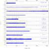 |
Fig. 1 Light curves of the eleven VLT runs in a wide photometric band obtained summing the g′ and r′ counts. The target’s counts are divided by the counts of the stable star. |
2.1. Sky stability on short time scales using a 8 m class telescope
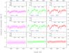 |
Fig. 2 Sky intensity fluctuations on time scales from tenths to tens of seconds (u′, g′ and r′ photometric bands). A section of the light curve of G 185-32 (18 May 2005), with a duration of 1 min, is represented in the upper panels, while the reference star is shown in the central panels. The average counts of each integration (8.8 ms) are reported. The lower panels show the intensity ratio (target’s counts divided by reference star’s counts). This figure shows that on time scales longer than about 1 s it is essential to have a reference star in order to reduce the sky fluctuations. However, for shorter time scales, the light curves of the target and the reference star are not coherent anymore, as we can see from the small panels representing a short section (only 2 s) of the same light curves. Note that the u′ band has a different vertical scale in all panels. |
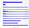 |
Fig. 3 Fourier amplitude spectra of the light curves of Fig. 1. For G 185-32 the high frequency tail, from 14.5 Hz to the Nyquist frequency at about 46.7 Hz, is not shown in this plot and does not contain any significant peak. The ordinate is in relative amplitude × 1000, which is equivalent to milli-modulation amplitude units (mma, 1 mma = 0.1% = 1000 ppm). For two stars, WD 1338-0023 and HS 1253+1033, a different vertical scale has been used. The peak near 3.3 Hz in the spectrum of HS 1253+1033 is a false detection (see text for details). |
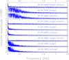 |
Fig. 4 Amplitude spectra of G 185-32 (detail of the low frequency part). The amplitude spectra of the target and reference star alone are also reported. As already seen in Fig. 2, these plots confirm that above about 1 Hz (where transparency variations cease) the mean noise of the amplitude spectrum is lower when we consider the target alone instead of using the flux ratio. |
In all our runs we see sky variations on time scales up to tens of minutes that can reach amplitudes of 10% and even more. In our best runs on HS 1443+2934 and L 19-2 these variations have much smaller intensities (few thousandths) and the flux remains constant within ~3% during the whole observation. Our data allow to test the sky stability also on much shorter time scales, down to tenths of seconds. An example is given in Fig. 2, where we see that the variability on time scales from seconds to tens of seconds resembles that of the typical transparency variations on longer time scales (minutes to hours). These variations are coherent at angular distances of 1–2 arcmin, as we see comparing target and reference star’s light curves. However, at higher frequencies (≳1 Hz), the spatial coherence is lost, as shown in the small panels of Fig. 2.
3. Search for periodicities
Figure 3 shows the amplitude spectra of the eleven runs in the g′+r′ band. The only significant peak at about 3.3 Hz in the spectrum of HS 1253+1033 is a false detection which appears also in the spectrum of the reference star alone. These amplitude spectra were calculated using the flux ratios (target’s counts divided by stable star’s counts). However, we have seen in Sect. 2.1 that differential photometry is useful only at frequencies lower than about 1 Hz (see Figs. 2 and 4). For this reason we calculated also the amplitude spectra of the eleven runs using only the target’s counts. Again we did not detected any significant peak in any of the spectra. Negative results were found also when using the data of the single u′, g′ and r′ photometric bands.
Looking at Fig. 3, we note an excess of power below ~2 Hz in all the three nights of observation on G 185-32, the brightest target of our sample. This excess, which is only marginally present in three other targets (L 19-2, GD 133 and HS 1443+2934), could be due in principle to tens of close modes with low amplitude. However, when we look in detail to the low frequency part of the spectra, we see that the low-amplitude peaks are different from night to night, contrary to what we would expect (Fig. 4). To test this hypothesis in greater depth, we can use one of the properties of the p-modes: the high-overtone modes should be almost equally spaced in frequency (a constant spacing is expected when the adiabatic sound speed is constant in a star with an homogeneous composition). An almost constant frequency spacing would be easily detected using correlation analysis or through Fourier transform (FT) of the amplitude spectrum (or FT2). For all our targets we have used both methods without detecting any significant peak. An example is given in Fig. 5, where FT2 and autocorrelation function of G 185-32 are shown and compared with those of a synthetic run containing a set of 20 equally spaced frequencies between 1.265 and 2.5 Hz with same amplitude (see caption of Fig. 5 for more details). With relative amplitudes equal to 2 × 10⁻⁴, no synthetic sinusoids are detected in the amplitude spectrum. With larger amplitudes of 4 × 10⁻⁴ (6 × 10⁻⁴), 8 out of 20 (20/20) sinusoids are found. With 4 × 10⁻⁴ (6 × 10⁻⁴) a significant peak is found also from correlation analysis at 6 σ (17 σ), while FT2 is less sensitive.
Another possibility that we have considered is that the p-modes are not seen because of short life times. With life times shorter than the observing runs, their amplitude in the Fourier spectrum would be reduced due to phase incoherence and they could escape detection. In order to verify also this possibility, we have divided each run in a number of subruns of at least 14 s each and calculated the amplitude spectrum of each subset. Then, an automated procedure has found all the peaks with an amplitude higher than 3 times the local noise. The local noise has been determined by fitting each amplitude spectrum with a (smooth) cubic spline; an example of cubic spline interpolation is shown in Fig. 5 (2nd column). This procedure has been repeated for different size of the subsets, starting from 1344 data points and increasing the size by a factor of ~2 at each iteration. The results for the three runs on G 185-32 are illustrated in Fig. 6. We see from this plot that only a few peaks with S/N ratio higher than 4σ are found but, also in this case, the same peaks are not detected in different subsets, as we would expect. Moreover, from autocorrelation analysis we do not obtain any indication of frequency spacing in these subsets. We conclude that also the possibility that the p-modes have very short life times is not supported by our observations. This conclusion is valid for all the targets of our sample.
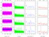 |
Fig. 5 Comparison between G 185-32 (18 May 2005, upper panels) and synthetic data. Each synthetic dataset was constructed by adding to the VLT data a sequence of 20 sinusoidal waves between 1.265 and 2.5 Hz, equally spaced in frequency (Δf = 0.065 Hz). All the 20 sinusoids have same relative amplitude of 2 × 10⁻⁴, 4 × 10⁻⁴ and 6 × 10⁻⁴ respectively. The various columns represent respectively: light curve with synthetic sinusoids superimposed (1), amplitude spectrum (2), amplitude spectrum of the amplitude spectrum or FT2 (3), autocorrelation function of the amplitude spectrum (4). The ordinate is given in relative amplitude × 1000 for Cols. 1 and 2, and in σ units for Cols. 3 and 4. The dashed lines show the 4σ detection threshold, which correspond to 4 times the average noise for Cols. 2 and 3 and to 4 times the standard deviation for Col. 4. In Col. 2 the mean noise was calculated using a (smooth) cubic spline interpolation in order to consider also the noise increase at low frequency due to transparency variations. |
4. Summary
We have not detected any significant peak in the amplitude spectra of nine DA white dwarfs near the DAV instability strip in the range of frequencies expected for the p-modes. The upper limits that we have obtained for the pulsation amplitudes are reported in Table 1, together with the main characteristics of the stars observed. Thanks to the high efficiency of the VLT-ULTRACAM system, our results move down the detection limit for the p-modes in DA white dwarfs to less than 0.1% for most of our targets. These limits are lower by a factor of about 2–3 (at same magnitude level) respect to previous findings (Robinson 1984) and the Nyquist frequencies are much larger, covering the whole range of frequencies expected for the p-modes. For G 185-32, the brightest target of our sample, an apparent excess of power is seen below ~2 Hz in all the three nights of observation but none of our analysis allows us to deduce that this apparent excess of power is indicative of the presence of p-modes. As shown by a simple simulation, a peak with a relative amplitude of 6 × 10⁻⁴ (3 × 10⁻⁴) in the frequency range 1–3 Hz (3–10 Hz) would have been easily detected in the amplitude spectrum of G 185-32.
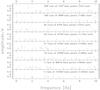 |
Fig. 6 Search for pulsations with life times shorter than the observing runs: each panel shows the peaks with amplitude higher than 3.3σ, detected in n subsets with same length, extracted from the three runs on G 185-32. Note that the detection limit varies from panel to panel as it goes with d − 1 / 2, where d is the duration of each subset. In this plot, the 4σ detection threshold goes from a relative amplitude of ~5 × 10⁻⁴ (lower panel) to about 6 × 10⁻³ (upper panel). Only for the online electronic version, the different colors refer to the different dates of the runs: green = 6 May, red = 7 May, blue = 18 May 2005. |
In our analysis we have considered various possibilities that could hide the p-modes (low amplitudes, very short life times) and applied various techniques that can help to bring the signal out of the noise. Using one of the properties of the high overtones p-modes, that should be almost equally spaced in frequency, we have searched for a constant frequency spacing through correlation analysis and Fourier transform of the amplitude spectrum (FT2), without finding significant results. Then we have divided each data set into several subsets of varying length and analyzed each subset independently, again without finding any trace of excited modes with very short life times.
Our results do not necessarily mean that the p-modes in DA white dwarfs stars are not excited at all. As the p-modes act mainly in the vertical direction, and vertical motions are limited by the huge gravity, a very low amplitude, below our detection limit, would not be surprising. We will examine in a subsequent publication with the help of detailed models how this can come about. The upper limits reported in this paper can help to constrain the nonadiabatic models of the DA white dwarfs, which have large uncertainties because of the convection.
Acknowledgments
ULTRACAM is supported by STFC grant PP/D002370/1. S.P.L. acknowledges the support of an RCUK Fellowship and STFC grant PP/E001777/1. G.F. acknowledges the contribution of the Canada Research Chair Program. A first observational search for p-mode pulsations in DA white dwarfs started in 2003, based on two observing runs at the SAO 6 m telescope using the MANIA instrument. Because of bad weather conditions, both the observing runs did not produced useful data. R.S. and M.P. wish to thank Grigory M. Beskin, Sergey V. Karpov and Vladimir L. Plokhotnichenko for the collaboration to the observations and for their kind hospitality at the 6 m SAO telescope in June 2004. Finally we thank the referee, Susan E. Thompson, for a careful reading of the manuscript and for useful suggestions.
References
- Bergeron, P., Fontaine, G., Billères, M., Boudreault, S., & Green, E. M. 2004, ApJ, 600, 404 [NASA ADS] [CrossRef] [Google Scholar]
- Cox, A. N., Hodson, S. W., & Starrfield, S. G. 1980, Proc. of the workshop on Nonradial and nonlinear stellar pulsation (Berlin: Springer-Verlag), 458 [Google Scholar]
- Dhillon, V. S., Marsh, T. R., Stevenson, M. J., et al. 2007, MNRAS, 378, 825 [NASA ADS] [CrossRef] [MathSciNet] [Google Scholar]
- Fontaine, G., & Brassard, P. 2008, PASP, 120, 1043 [NASA ADS] [CrossRef] [Google Scholar]
- Fontaine, G., Brassard, P., Charpinet, S., Quirion, P.-O., & Randall, S. K. 2010, in White Dwarfs, Monograph Series sponsored by the Royal Astronomical Society, ed. R. Napiwotzki, & M. Burleigh, Springer, in press [Google Scholar]
- Gianninas, A., Bergeron, P., & Fontaine, G. 2005, ApJ, 631, 1100 [NASA ADS] [CrossRef] [Google Scholar]
- Gianninas, A., Bergeron, P., & Fontaine, G. 2007, ASP Conf. Ser., 372, 577 [NASA ADS] [Google Scholar]
- Hansen, C. J., Winget, D. E., & Kawaler, S. D. 1985, ApJ, 297, 544 [NASA ADS] [CrossRef] [Google Scholar]
- Kawaler, S. D. 1993, ApJ, 404, 294 [NASA ADS] [CrossRef] [Google Scholar]
- Kawaler, S. D., Bond, H. E., Sherbert, L. E., & Watson, T. K. 1994, AJ, 107, 298 [NASA ADS] [CrossRef] [Google Scholar]
- Koester, D., Napiwotzki, R., Christlieb, N., et al. 2001, A&A, 378, 556 [NASA ADS] [CrossRef] [EDP Sciences] [Google Scholar]
- Landolt, A. U. 1968, ApJ, 153, 151 [NASA ADS] [CrossRef] [Google Scholar]
- Littlefair, S. P., Dhillon, V. S., Marsh, T. R., et al. 2008, MNRAS, 391, L88 [NASA ADS] [Google Scholar]
- Mukadam, A. S., Mullally, F., Nather, R. E., et al. 2004, ApJ, 607, 982 [NASA ADS] [CrossRef] [Google Scholar]
- Ostriker, J. P. 1971, ARA&A, 9, 353 [NASA ADS] [CrossRef] [Google Scholar]
- Robinson, E. L. 1984, AJ, 89, 1732 [NASA ADS] [CrossRef] [Google Scholar]
- Saio, H., Winget, D. E., & Robinson, E. L. 1983, ApJ, 265, 982 [NASA ADS] [CrossRef] [Google Scholar]
- Silvotti, R., Voss, B., Bruni, I., et al. 2005, A&A, 443, 195 [NASA ADS] [CrossRef] [EDP Sciences] [Google Scholar]
- Silvotti, R., Pavlov, M., Fontaine, G., Marsh, T., & Dhillon, V. 2006, MmSAI, 77, 486 [NASA ADS] [Google Scholar]
- Silvotti, R., Pavlov, M., Fontaine, G., et al. 2010, A&A, in preparation (Paper II) [Google Scholar]
- Starrfield, S., Cox, A. N., Hodson, S. W., & Clancy, S. P. 1983, ApJ, 269, 645 [NASA ADS] [CrossRef] [Google Scholar]
- Vauclair, G. 1971, Proc. of the on White Dwarfs, ed. W. J. Luyten (Dordrecht: Springer-Verlag), IAU Symp., 42, 145 [Google Scholar]
- Winget, D. E., & Kepler, S. O. 2008, ARA&A, 46, 157 [NASA ADS] [CrossRef] [EDP Sciences] [Google Scholar]
All Tables
All Figures
|
Fig. 1 Light curves of the eleven VLT runs in a wide photometric band obtained summing the g′ and r′ counts. The target’s counts are divided by the counts of the stable star. |
| In the text | |
|
Fig. 2 Sky intensity fluctuations on time scales from tenths to tens of seconds (u′, g′ and r′ photometric bands). A section of the light curve of G 185-32 (18 May 2005), with a duration of 1 min, is represented in the upper panels, while the reference star is shown in the central panels. The average counts of each integration (8.8 ms) are reported. The lower panels show the intensity ratio (target’s counts divided by reference star’s counts). This figure shows that on time scales longer than about 1 s it is essential to have a reference star in order to reduce the sky fluctuations. However, for shorter time scales, the light curves of the target and the reference star are not coherent anymore, as we can see from the small panels representing a short section (only 2 s) of the same light curves. Note that the u′ band has a different vertical scale in all panels. |
| In the text | |
|
Fig. 3 Fourier amplitude spectra of the light curves of Fig. 1. For G 185-32 the high frequency tail, from 14.5 Hz to the Nyquist frequency at about 46.7 Hz, is not shown in this plot and does not contain any significant peak. The ordinate is in relative amplitude × 1000, which is equivalent to milli-modulation amplitude units (mma, 1 mma = 0.1% = 1000 ppm). For two stars, WD 1338-0023 and HS 1253+1033, a different vertical scale has been used. The peak near 3.3 Hz in the spectrum of HS 1253+1033 is a false detection (see text for details). |
| In the text | |
|
Fig. 4 Amplitude spectra of G 185-32 (detail of the low frequency part). The amplitude spectra of the target and reference star alone are also reported. As already seen in Fig. 2, these plots confirm that above about 1 Hz (where transparency variations cease) the mean noise of the amplitude spectrum is lower when we consider the target alone instead of using the flux ratio. |
| In the text | |
|
Fig. 5 Comparison between G 185-32 (18 May 2005, upper panels) and synthetic data. Each synthetic dataset was constructed by adding to the VLT data a sequence of 20 sinusoidal waves between 1.265 and 2.5 Hz, equally spaced in frequency (Δf = 0.065 Hz). All the 20 sinusoids have same relative amplitude of 2 × 10⁻⁴, 4 × 10⁻⁴ and 6 × 10⁻⁴ respectively. The various columns represent respectively: light curve with synthetic sinusoids superimposed (1), amplitude spectrum (2), amplitude spectrum of the amplitude spectrum or FT2 (3), autocorrelation function of the amplitude spectrum (4). The ordinate is given in relative amplitude × 1000 for Cols. 1 and 2, and in σ units for Cols. 3 and 4. The dashed lines show the 4σ detection threshold, which correspond to 4 times the average noise for Cols. 2 and 3 and to 4 times the standard deviation for Col. 4. In Col. 2 the mean noise was calculated using a (smooth) cubic spline interpolation in order to consider also the noise increase at low frequency due to transparency variations. |
| In the text | |
|
Fig. 6 Search for pulsations with life times shorter than the observing runs: each panel shows the peaks with amplitude higher than 3.3σ, detected in n subsets with same length, extracted from the three runs on G 185-32. Note that the detection limit varies from panel to panel as it goes with d − 1 / 2, where d is the duration of each subset. In this plot, the 4σ detection threshold goes from a relative amplitude of ~5 × 10⁻⁴ (lower panel) to about 6 × 10⁻³ (upper panel). Only for the online electronic version, the different colors refer to the different dates of the runs: green = 6 May, red = 7 May, blue = 18 May 2005. |
| In the text | |
Current usage metrics show cumulative count of Article Views (full-text article views including HTML views, PDF and ePub downloads, according to the available data) and Abstracts Views on Vision4Press platform.
Data correspond to usage on the plateform after 2015. The current usage metrics is available 48-96 hours after online publication and is updated daily on week days.
Initial download of the metrics may take a while.