| Issue |
A&A
Volume 525, January 2011
|
|
|---|---|---|
| Article Number | A47 | |
| Number of page(s) | 18 | |
| Section | Stellar structure and evolution | |
| DOI | https://doi.org/10.1051/0004-6361/201015299 | |
| Published online | 30 November 2010 | |
U-band study of the accretion properties in the σ Orionis star-forming region⋆,⋆⋆
1
Osservatorio Astrofisico di Arcetri, INAF, Largo E. Fermi 5,
50125
Firenze,
Italy
e-mail: This email address is being protected from spambots. You need JavaScript enabled to view it.
2
Università di Firenze, Dipartimento di Astronomia,
Largo E. Fermi 2, 50125
Firenze,
Italy
3
ESO, Karl-Schwarszchild Strasse 2, 85748
Garching bei München,
Germany
Received: 29 June 2010
Accepted: 9 October 2010
Abstract
This paper presents the results of an U band survey with FORS1/VLT of a large area in the σ Ori star-forming region. We combine the U-band photometry with literature data to compute accretion luminosity and mass accretion rates from the U-band excess emission for all objects (187) detected by Spitzer in the FORS1 field and classified by Hernandez et al. as likely members of the cluster. The sample stars range in mass from ~0.06 to ~1.2 M⊙; 72 of them show evidence of disks and we measure mass accretion rates Ṁacc between <10-11 and few 10-9 M⊙/y, using the colors of the diskless stars as photospheric templates. Our results confirm the dependence of Ṁacc on the mass of the central object, which is stronger for low-mass stars and flattens out for masses larger than ~0.3 M⊙; the spread of Ṁacc for any value of the stellar mass is ~2 orders of magnitude. We discuss the implications of these results in the context of disk evolution models. Finally, we analyze the relation between Ṁacc and the excess emission in the Spitzer bands, and find that at Ṁacc ~ 10-10 M⊙/y the inner disks change from optically thin to optically thick.
Key words: stars: formation / accretion, accretion disks / open clusters and associations: individual:σOrionis
Based on observations collected at the European Southern Observatory, Chile. Program 082.C-0313(A).
Appendices are only available in electronic form at http://www.aanda.org
© ESO, 2010
1. Introduction
In recent years, our knowledge of the properties of young stars in several star-forming regions has made enormous progress. In particular, Spitzer observations have provided new information on the IR properties of circumstellar disks, and the discussion on how disks evolve in time has gained new momentum. In addition to the classical viscous evolution, which dissipates disks by accreting their matter onto the central stars, other processes such as gravitational instabilities, photoevaporation by X-ray and UV radiation of the central star (Hollenbach et al. 2000; Gorti & Hollenbach 2009), and planet formation (Dullemond et al. 2009) have been recognized to be important. Photoevaporation and planet formation may both shape the SED (spectral energy distribution) of so-called transitional disks, which have very low emission in the near- and mid-IR and strong excess emission at longer wavelengths (Calvet et al. 2002, 2005; D’alessio et al. 2006; Currie et al. 2009). In all cases, disks seem to come in all varieties: it is clear that neither time nor the mass of the system control them uniquely, and it seems very likely that disk properties and evolution depend also on the initial conditions, i.e., on the properties of the molecular core from which the star+disk system forms (Hartmann et al. 1998, 2006; Dullemond et al. 2006; Clarke 2007; Vorobyov & Basu 2009).
An important contribution to this discussion comes from measurements of the mass accretion rate for well characterized samples of stars. However, there are only few systematic determinations of the mass-accretion rates in large samples of objects within the same star-forming regions, covering a large range of central masses, with well measured SEDs and complete to include also diskless stars, limited so far to ρ-Oph (Natta et al. 2006) and Tr 37 (Sicilia-Aguilar et al. 2010).
In this paper, we add a third region, σ Ori, to the list. The σ Ori cluster is ideally suited for this kind of study. It contains more than 300 young stars, ranging in mass from the bright, massive multiple system σ Ori itself (the spectral type of the brightest star is O9.5V, Caballero 2007) to brown dwarfs. It is located at a distance of ~360 pc (Hipparcos distance  pc for the O9.5V star Brown et al. 1994; Perryman et al. 1994) and has an age of ~3 Myr (Zapatero-Osorio et al. 2002; Oliveira et al. 2004). The region has negligible extinction (Bejar et al. 1999; Oliveira et al. 2004), and has been extensively studied in the optical, X-ray and infrared (e.g., Kenyon et al. 2005; Zapatero-Osorio et al. 2002; Jeffries et al. 2006; Franciosini et al. 2006; Hernandez et al. 2007; Caballero et al. 2007; Wolk 1996). Hernandez et al. (2007) have obtained Spitzer images of a large area in σ Ori in the four IRAC bands and with MIPS at 24 μm; they find 336 candidate members, of which 66% are class III stars and 34% show evidence of disks.
Accretion rates have been obtained by Gatti et al. (2008) for 35 objects in σ Ori from the luminosity of the near-IR hydrogen line Paγ; they found mass accretion rates lower on average than in younger regions. However, their sample was small and limited in mass (0.12–0.5 M⊙). In this paper, we present the results for a much larger and better characterized sample from Hernandez et al. (2007). We measure mass accretion rates from the U-band excess emission, which originates in the accretion shock where accreting matter impacts on the stellar surface (Gullbring et al. 1998; Calvet & Gullbring 1998). The correlation between the U-band excess luminosity and the accretion luminosity has been established both empirically (Gullbring et al. 1998; Herczeg & Hillenbrand 2008) and theoretically (Calvet & Gullbring 1998). The U-band excess is an excellent proxy of the accretion luminosity, which allows obtaining reliable values of the mass accretion rate for large samples of stars using little observing time when, as in σ Ori, the extinction is negligible. It very well complements measurements obtained from other tracers, such as the IR hydrogen recombination line luminosities (see the discussion in Herczeg & Hillenbrand 2008).
The paper is organized as follows: observations and data reduction are described in Sect. 2, the properties of the sample are derived in Sects. 3, in 4 we discuss the method used to derive the accretion properties. The results are discussed in Sects. 5 and 6. Three appendices present additional material on: the recomputation of accretion rates in ρ-Oph with the new distance and evolutionary tracks; the accretion properties of BD candidates beyond the Spitzer sample; and the properties of transitional and evolved disks in our sample.
2. Observations and data analysis
2.1. U-band photometry
We have performed a U-band survey that covers a total field of ~1000 arcmin2 in the σ Orionis cluster. Observations were carried out with FORS1 mounted on the UT2 telescope at the VLT using  filter and were performed in service mode during seven nights from October 2008 to March 2009. All the nights were photometric, with seeing in the range 0.6–1.5′′. We observed 28 fields (FOV 6′̣8 × 6′̣8) in σ Ori with an exposure time of 900 s each. The distribution of the pointings obtained with FORS1 is shown in Fig. 1 and the log of the observation is provided in Table 1. The long exposure time on each field allowed us to reach a U-band limiting magnitude of ~23; objects brighter than U ~ 17 mag are saturated. The fields around the two brightest stars of the quintuplet system containing σ Ori (within 0.2 pc projected distance) had to be excluded because of to light contamination.
Journal of observations. RA and Dec refer to the pointing center.
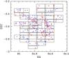 |
Fig. 1 Fields in the σ Ori cluster that have been imaged with FORS1 (solid boxes). Crosses (blue) show class III stars, circles (red) class II, TD and EV object, as classified by Hernandez et al. (2007). |
2.2. Data reduction
The data were reduced using standard procedures including bias subtraction and flat fielding within the IRAF1 package. We performed aperture photometry with the PHOT task in the APPHOT package, and using noao.digiphot.daophot routines for the photometry extraction. The stellar density was generally low enough to make aperture photometry acceptable. The IRAF routine MKAPFILE was used to determine and apply aperture corrections based on ensemble averages of stars in each separate frame. Astrometry correction was done to center the telescope coordinates. Photometric standard stars from Landolt (1992) and Persson et al. (1998) were observed at least once during each night and were used to flux-calibrate the images using the task PHOTCAL and to set the zero point magnitudes of each observing night and for both chips. Aperture photometry was performed using ten different apertures per image (0.5, 0.6, 0.7, 0.8, 0.9, 1.0, 1.25, 1.5, 2.0, 3.0 times the average FWHM). The inner radius of the sky annulus, which allowed us to define the sky brightness, was 10 times the average FWHM, while the width of the annulus was fixed at 10 pixels.
The uncertainties on the U-band magnitudes obtained are on the order of ± 0.1 mag. They are dominated by systematic errors, the biggest of which is the error on the zero point magnitude (about 0.08 mag), which affects all measurements in the same manner; a second systematic term, on the order of 0.01 mag, is due to the color term correction with respect to the filter. Random errors owing to the aperture photometry technique used to derive the stellar flux and the sky brightness are also very small.
2.3. U-band variability
Young pre-main sequence stars are known to be variable, with timescale from hours to several days (e.g., Gomez de Castro et al. 1998; Hillenbrand et al. 2009; Briceño et al. 2001; Sicilia-Aguilar et al. 2005a,b). The U-band variability is probably related to variations of the accretion rate, and, although a proper study is well outside the scope of this paper, it is interesting to estimate how large an effect this is likely to be.
In our FORS1 data there are 30 objects that lie at the superposition of two different fields and have therefore been observed twice, with separations that range between few days and few months. Of these, 19 are Class III stars and show no variability within the photometric uncertainty. Of the 11 Class II objects, 5 show no variability, 5 have variations between 0.15 and 0.4 mag, and one (SO866) has two measurements which differ by about 0.8 mag. This is similar to what is observed in other star-forming regions (see, e.g., Sicilia-Aguilar et al. 2010, and references therein).
Variability on a much longer time base can be checked by comparing our sample to that observed by Wolk (1996), where the observations were carried out in January 1996 with the 1 m telescope CTIO. The two samples have ~30 class II stars in common (see Fig. 2). The comparison between the U band magnitude determinations shows a ΔU variation of at most 0.5 mag, not different from what we observe on a shorter timescale.
A difference of 0.5 mag in the measured U-band magnitude corresponds to a Lacc and Ṁacc difference of a factor of at most two (see Sect. 4). This can be important when discussing individual objects. However, if the accretion properties of a large sample of stars are considered, it can only cause a moderate spread in the accretion values.
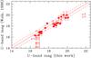 |
Fig. 2 U-band magnitude from Wolk (1966) and this work. Dashed lines correspond to an interval of ± 0.5 mag. |
2.4. Spectroscopy
Among the objects observed with FORS1, six have also optical spectroscopy obtained with SARG@TNG. We obtained spectroscopic observations in 2009 at the Telescopio Nazionale Galileo (TNG) during three nights from 27 to 29 January. The SARG spectrograph attached to the 3.58 m telescope was used with the 2048 × 4096 CCD detector (pixel size = 13.5 μm) and the Yellow Grism CD#3 as cross-disperser. This allowed us to cover ~6200–8000 Å wavelength range. We used the slit #1 obtaining R = 29000 as spectral resolution.
The data reduction was performed by using the echelle task of the IRAF package following the standard steps of background subtraction, division by a flat-field spectrum given by a halogen lamp, wavelength calibration using emission lines of a Thorium-Argon lamp, and sky subtraction.
With exposure times of 10–30 min we achieved signal-to-noise ratios (S/N) in the range 10–15 in the lithium line λ6708 Å region, depending on airmass and sky conditions. Each star was observed 1–3 times. All the spectra acquired per star were shifted in wavelength for the heliocentric correction and then co-added obtaining a S/N ratio in the continuum around 20.
3. The observed sample
Table C.2 gives the measured U-band magnitude of all the objects in the FORS fields listed as σ Ori members by Hernandez et al. (2007) based on optical and near-IR photometry. This sample of 187 objects (out of 336 members) is our basic sample and will be discussed below.
The Hernandez et al. (2007) sample spans the mass range from ~0.06 to 2–3 M⊙, and is practically complete above 0.1 M⊙. Based on the SED in the IRAC spectral range (from 3.6 μm to 8.0 μm) the Spitzer sources are divided in in class II stars, pre-main sequence stars with IR excess typical of optically thick disks (classical TTauri stars CTTs or CII), class III stars, with typical colors of stellar photospheres (weak-line T Tauri stars WTTs or CIII), and stars with non-classical disks, in turns divided in “evolved disks” (EV), with small excess emission at all infrared wavelengths, and “transitional disks” (TD), which have zero or very low emission in the near infrared but normal excess at longer wavelengths. Below we will refer to class II, TD, and EV objects as “disk objects”.
Our sample includes 115 class III members, and 72 objects with evidence of disks. Among these, there are 54 class II stars, 4 TD (out of the 7 possibly identified by Hernandez et al. 2007), and 14 EV disks. Of the 72 stars with disks, 54 are detected in the U-band, 6 are non-detections, and 12 are saturated. Out of the 115 class III stars, 83 are detected, 7 are not, and 25 are saturated.
The spatial distribution of the observed sample is shown in Fig. 1.
3.1. Stellar properties
Spectroscopically determined spectral types exist for a small fraction of the σ Ori objects only (Zapatero-Osorio et al. 2002; Barrado y Navascues et al. 2003; Muzerolle et al. 2003). Therefore, we determine the stellar parameters (effective temperature, luminosity, mass, and radius) of all objects in a homogeneous way from multi-color photometry.
Table C.2 reports for each object broad-band magnitudes collected from the literature. The optical photometry is from Sherry et al. (2004); Zapatero-Osorio et al. (2002); Kenyon et al. (2005); Béjar et al. (2001) and Wolk (1996). The JHK magnitudes are taken from the Two Micron All Sky Survey (2MASS) (Cutri et al. 2003). The magnitudes in the four channels of the Infrared Array Camera (IRAC; 3.8–8.0 μm) and the first channel of the Multiband Imaging Photometer for Spitzer (MIPS; 24 μm) are from Hernandez et al. (2007). When two or more magnitude determinations for the same band were available, we choose, if possible, measurements obtained by the same author.
We derived the effective temperatures of each star by comparing the observed magnitudes to the synthetic colors computed from the model atmosphere of Baraffe et al. (1998) for log g = 4.0 and the appropriate filter passband and zero fluxes. Luminosities were then computed using the I-band magnitude and the bolometric correction for ZAMS stars and the Teff – spectral type correlation of Kenyon & Hartmann (1995) and Luhman et al. (2003). We assumed a distance of D = 360 pc, and negligible extinction in all bands (Brown et al. 1994; Bejar et al. 1999).
We performed two checks on the Teff estimates. In a first test, we compared the values derived from the model atmosphere synthetic colors with those obtained by comparing the observed colors (V − R), (V − I) and (R − I) to those of ZAMS stars. The differences are within 150 K for 90% of the stars, with a slight systematic tendency toward higher values for model atmosphere estimates. A second test is given by the comparison of our estimates of Teff with the spectroscopic determination derived from low- and medium-resolution observations. In a sample of 22 objects in the range ~3200–4000 K we find differences of ± 150 K at most.
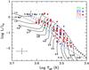 |
Fig. 3 Location of the observed objects (class III, class II, and objects with “non-classical” disks, as labeled) on the HR diagram. Evolutionary tracks and isochrones are taken from Baraffe et al. (1998). Stellar masses and ages are labeled. The horizontal bar refers to the error on the effective temperature, the vertical bar reflects the error of the bolometric correction of the ZAMS stars related to the error on the effective temperatures. |
Accretion properties of the class II objects and objects with transitional and evolved disks.
The distribution of the stars in the HR diagram is shown in Fig. 3 with the evolutionary tracks and isochrones from Baraffe et al. (1998). The sample covers the mass range between ~1.2 to ~0.05 M⊙; both the lower and the higher mass limit reflect the sensitivity limit of the Spitzer survey (see discussion in Hernandez et al. 2007). The median age is about 3 My, with a rather large spread, which is similar for Class II and Class III objects. This spread also remains when only radial velocity confirmed members are considered (Sacco et al. 2008; Kenyon et al. 2005). The issue of the spread in age in σ Ori as well as in other young star-forming regions has been discussed in several papers (e.g. Hillenbrand 2009, and references therein) and further discussion is beyond the purpose of this paper. Note, however, that the error bars may be quite large and affect the age estimates significantly.
The stellar parameters of all Class II objects are summarized in Table 2.
4. Mass accretion rate
Matter accreting from the disk onto the star, channeled along field lines, shocks at the stellar surface. About half of the accretion luminosity is released with a typical color temperature of ~104 K, i.e., much hotter than the stellar photosphere (Hartigan et al. 1991; Gullbring & Calvet 1998). The resulting excess emission is clearly detected at short wavelengths, in the U-band in particular. It has been shown (Gullbring & Calvet 1998; Herczeg & Hillendrand 2008) that the U-band excess luminosity is an accurate proxy of the accretion luminosity, which can be reliably used to measure Lacc for T Tauri stars and BDs.
4.1. Class III sources
In order to measure the excess of luminosity in U-band for a given object, we need to know the measured U-band luminosity and the expected photospheric U band luminosity for a non-accreting star with the same parameters. This is not trivial, as young stars tend to have a significant level of chromospheric activity that causes continuum emission at short wavelengths; this is not related to accretion and must, therefore, be counted as “photospheric” contribution for our purpose.
We take advantage of the large number of Class III stars in our sample to define the typical colors of non-accreting young stars. Figure 4 plots the class III (U − J), (U − I), (U − R) and (U − V) colors as a function of the effective temperature of the star. For each color index, there is a tight correlation with the effective temperature; the solid lines show the best fits, the dashed lines the 2σ errors, which are ~0.5 mag at most. Hereafter, we will refer to the ± 2σ as the photospheric strip. Note that while (U − J) increases with Teff, (U − V) slightly decreases.
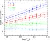 |
Fig. 4 Colors of Class III stars vs. effective temperature. Blue horizontal lines plot (U − J), red crosses (U − I), green 45 deg lines (U − R), cyan –45 deg lines (U − V), as labeled. The solid lines show the best fit, the dashed lines ± 2σ. In the text, we will define the region between the dashed lines as the photospheric strip. (A color version of this figure is available in the online journal.) |
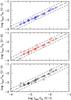 |
Fig. 5 Values of the accretion luminosity derived from (U − J), (U − R), (U − V) vs. the value derived from (U − I), as described in the text for a sub-sample of 30 objects. The dashed lines correspond to ± 0.5 in log Lacc. |
4.2. Disk sources
To derive the U-band excess emission in class II objects we assign to each of them the photospheric colors of class III stars of the same Teff, according to the correlations shown in Fig. 4; we assume that there is negligible excess emission in the V,R,I, and J band and derive the U-band excess from the difference between the observed and the photospheric colors. We use (U − I), as I-band magnitudes are available for all stars in our sample (see Table C.2), using the relation:  (1)where (U − I)obs are the observed (U − I) color, and (U − I)phot is the assigned photospheric color.
We define as accreting all stars with ΔUexcess larger than the 2σ uncertainties of the photospheric colors, as derived in Sect. 4.1. Class II stars with colors within the class III photospheric strip will be considered not-accretors and we can only assign upper limits to the accretion luminosity and mass accretion rate. We choose the 2σ uncertainty as good compromise not to loose low-accreting stars. After defining the accreting or non-accreting stars, we computed the excess flux in the U-band as:  (2)where F0,U is the zero point flux in the U-band.
Figure 5 shows the comparison between the accretion luminosities computed from (U − I) vs. those derived from (U − J), (U − R) and (U − V), respectively, for all objects with available photometry. The derived Lacc are the same within a factor ~3 for all objects, and for 70% of them the agreement is within a factor 1.5. These results support several aspects of our procedure: within the above uncertainties: firstly, our assumption that reddening is negligible at all wavelengths; secondly, that there is negligible excess emission in V,R,I, and J; thirdly, since the photometric data are collected from the literature and are not simultaneous, that variability is not the major limiting factor in deriving the accretion properties (although it may introduce some scatter in the measurements).
We use the (U − I) color to define the accretion rates. Assuming an uncertainties in U-band of 0.5 mag we estimate an error on the U-band luminosities of a factor 3 at most.
4.3. Accretion rate
The U-band luminosity obtained from the excess flux in the U-band (Eq. (2)) is converted into total accretion luminosity Lacc, which is roughly the amount of energy released by gas that accretes onto the star, using the approximately linear relation derived for T Tauri stars (Gullbring & Calvet 1998) and brown dwarfs (Calvet & Gullbring 1998; Herczeg & Hillendrand 2008):  (3)Knowing M∗, R∗ and the accretion luminosity Lacc we derive the mass accretion rate
  with the relation
  (4)where G is the universal gravitational constant and the factor
  is estimated by assuming that the accretion gas falls onto the star from the truncation radius of the disk (Rin ~5 R∗; Gullbring et al. 1998).
Table 2 reports 72 actual values of Ṁacc. Thirty stars have Ṁacc detection. In 30 cases, we can only estimate upper limits to Ṁacc. Of these, 6 are objects with U-band emission below our detection limit, while 24 have colors within the photospheric strip (Sect. 4.2). Eight stars have expected U-band photospheric emission brighter than our saturation limit (labeled “sat”), and 4 stars have U < 17 mag, but colors with a lower limit than Ṁacc can be safely estimated because their photospheric contribution is lower than the saturation limit, and the upper limit in the U-band can be only due to the accretion process.
The lowest values of Ṁacc we can estimate range from ~10-11 M⊙/y for very low, cold objects to few 10-10 M⊙/y for solar-mass stars. This trend occurs because the minimum detectable value of Ṁacc from U-band photometry depends not only on the depth of the photometry, but also on the physical properties of the star, and on how well one can estimate the photospheric flux. Indeed, this is at present the major limiting factor.
The uncertainties on individual measurements of Lacc and Ṁacc are quite large. They come from the combination of photometric errors and variability, the definition of the class III colors, the adopted relation between the U-band excess luminosity and the accretion luminosity, and between the latter and Ṁacc and the uncertainty on the value of R∗/M∗ (see also Sicilia-Aguilar et al. 2010). Some of these uncertainties have been discussed in the previous sections, while others, e.g., the differences owing to different evolutionary tracks, by other authors (Fang et al. 2009). Our estimate is that in general Ṁacc is known with an uncertainty of a factor 3–5.
5. Results
Detectable values of accretion luminosity and mass accretion rate were obtained for 42% of disk objects. Another 42% have upper limits in accretion luminosity and mass accretion rate. The remaining 16% have lower limits (see Sect. 4.3).
Gatti et al. (2008) compute Lacc from the luminosity of the hydrogen recombination line Paγ, following the procedure described by Natta et al. (2006).
Figure 6 compares the values of Lacc derived with the two different methods (U-band excess emission and Paγ recombination line respectively) for the 12 stars we have in common; it agrees well. Another nine stars of the Gatti et al. (2008) sample are class II objects and were observed with Spitzer. We could not observe these stars either because they are outside the FORS fields, or because they are close to the brighter stars of the σ Ori quintuplet system. We added these nine stars to our sample. In Table. 3 the properties of the sub-sample derived from Gatti et al. (2008) are listed. For these stars we recomputed the stellar properties adopting the Baraffe et al. (1998) evolutionary tracks, in the same way as for the present sample.
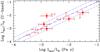 |
Fig. 6 Comparison between Lacc computed from Paγ (Gatti et al. 2008) and Lacc obtained from U-band photometry for stars in common. The dashed line refers to the same value of Lacc, the dashed-dotted lines to ± 0.5 in log Lacc. |
Accretion properties of the class II objects taken from Gatti et al. (2008).
Figures 7–10 show the relations between the accretion properties and different physical and morphological properties of the observed sample.
In Fig. 7 we specifically plot the accretion luminosity as a function of the stellar luminosity for all class II objects; transitional and evolved disks are shown by different symbols. The figure shows that very few stars have Lacc larger than 0.1 Lstar, and that most of them have values well below this limit. The accretion luminosities for the detected sources range mainly from ~10-2 L⊙ to ~10-4 L⊙. For any given L∗ there is a large range of measured Lacc that does not seem to vary significantly with L∗ .
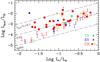 |
Fig. 7 Accretion luminosity as a function of the stellar luminosity for class II, EV, and TD disks, as labeled. The dashed lines show Lacc/Lstar = 0.001, 0.01, and 0.1, respectively. The crosses surronded by a circle are the class II stars included here from the Gatti et al. (2008) sample, and listed in Table 3. Different colors for lower and upper limits can be distinguished in the online version of the journal. |
Figure 8 shows the mass accretion rate of class II stars as function of M∗. The data show a clear trend of increasing Ṁacc with increasing M∗. Including upper and lower limits as actual detections, we find  with ASURV (Astronomy Survival Analysis Package, Feigelson & Nelson 1985). The trend is confirmed using two different methods (the EM algorithm and the BJ algorithm) within the ASURV package. The slope became flatter when we excluded the upper and lower limits in the analysis, but remained still within the uncertainties. From this plot we can clearly also see the large spread in (about two orders of magnitude) for any value of M∗.
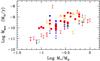 |
Fig. 8 Mass accretion rate as function of stellar mass. Symbols as in Fig. 7. (A color version of this figure is available in the online journal.). |
In Fig 9 we plot the mass accretion rates versus the age of the stars.
Finally, in Fig. 10 we plot the mass accretion rates as function of the projected distance from the central and bright O9.5 star σ Ori. We do not find any correlation between the mass accretion rates or the disk morphologies and the distance from σ Ori; it seems that the vicinity of the O9.5 star does not affect the disk properties significantly (see also Hernandez et al. 2007). Rigliaco et al. (2009) studied in detail one object (SO587), which has a projected distance of 0.3 pc; based on literature U-band photometry and optical spectroscopy, they proposed that its disk is in the process of being photoevaporated, either by σ Ori or by its own central star. There are six additional objects with a projected distance of ≲ 0.3 pc from σ Ori with a Ṁacc range of more than a factor of ten, and it would be interesting to obtain high-resolution optical spectra to study wind diagnostics such as the optical forbidden lines of [SII], [NII] and [OI].
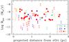 |
Fig. 10 Mass accretion rates versus projected distance from the bright stars σ Ori in parsec. (A color version of this figure is available in the online journal.) |
We caveat that in both Figs. 9 and 10 we did not divide stars in mass bins (which would result in too low number statistics); thus the relationship of Ṁacc vs. M∗ seen in Fig. 8 might mask possible trends between Ṁacc and age or Ṁacc and the projected distance from σ Ori.
6. Discussion
6.1. as function of M∗ and time
The distribution of mass accretion rates in a star-forming region traces the physical processes that control disk formation and evolution over the lifetime of the region, as well as the initial conditions, i.e., the mass and angular momentum distribution of the molecular cores from which the stars form. It is a snapshot in time, which needs to be compared to models that follow disk formation and evolution up to the age of the region (e.g., Dullemond et al. 2006; Vorobyov & Basu 2008, 2009).
It has been known for some years that mass accretion rates increase on average with the mass of the central object. In σ Ori, a logarithmic linear correlation over the whole mass range, Ṁacc  (Sect. 5), is similar within the uncertainties to what has found in Taurus (Calvet et al. 2004) and Ophiuchus (Natta et al. 2006), but flatter than in L1630N and L1641 (Fang et al. 2009). However, in σ Ori the trend seems to be flatter for higher mass stars than for lower mass objects, as also noted by Vorobyov & Basu (2008) in a compilation of all known Ṁacc values in various star-forming regions. This is shown in Fig. 11, which plots median values of Ṁacc as function of M∗ for Class II and TD disks. All M∗ intervals above 0.1 M⊙ contain roughly the same number of stars (12–20). The values plotted in Fig. 11 treat upper and lower limits as actual detections; if we make the alternative assumption that lower (upper) limits are all smaller (larger) than the lowest (highest) measured value in the bin, the changes are very small; however, the large number of limits and the small number of objects in each bin make it meaningless to derive values for the upper and lower quartiles, to characterize the spread of Ṁacc seen in Fig. 8. The mass interval below 0.1 M⊙ contains only two detections and six upper limits to Ṁacc, and the value in Fig. 11 (Log Ṁacc =
–10.8 M⊙/y) should be considered as an upper limit to the median. The deficit of relatively strong accretors among the σ Ori BDs is confirmed by the analysis of a much larger (40 objects, see Appendix B), optically selected sample of very low-mass stars and BDs (Lodieu et al. 2009), included in our U-band survey, which contains only five objects with Log Ṁacc > −10.8 M⊙/y, two of which are also in the Hernandez et al. (2007) Spitzer sample.
(Sect. 5), is similar within the uncertainties to what has found in Taurus (Calvet et al. 2004) and Ophiuchus (Natta et al. 2006), but flatter than in L1630N and L1641 (Fang et al. 2009). However, in σ Ori the trend seems to be flatter for higher mass stars than for lower mass objects, as also noted by Vorobyov & Basu (2008) in a compilation of all known Ṁacc values in various star-forming regions. This is shown in Fig. 11, which plots median values of Ṁacc as function of M∗ for Class II and TD disks. All M∗ intervals above 0.1 M⊙ contain roughly the same number of stars (12–20). The values plotted in Fig. 11 treat upper and lower limits as actual detections; if we make the alternative assumption that lower (upper) limits are all smaller (larger) than the lowest (highest) measured value in the bin, the changes are very small; however, the large number of limits and the small number of objects in each bin make it meaningless to derive values for the upper and lower quartiles, to characterize the spread of Ṁacc seen in Fig. 8. The mass interval below 0.1 M⊙ contains only two detections and six upper limits to Ṁacc, and the value in Fig. 11 (Log Ṁacc =
–10.8 M⊙/y) should be considered as an upper limit to the median. The deficit of relatively strong accretors among the σ Ori BDs is confirmed by the analysis of a much larger (40 objects, see Appendix B), optically selected sample of very low-mass stars and BDs (Lodieu et al. 2009), included in our U-band survey, which contains only five objects with Log Ṁacc > −10.8 M⊙/y, two of which are also in the Hernandez et al. (2007) Spitzer sample.
The flattening of the Ṁacc vs. M∗ relation at higher masses is very clear. Vorobyov & Basu (2009) compute numerical models of the collapse of a distribution of prestellar cores that include the formation and evolution of circumstellar disks and follow it for 3 My, roughly the age of σ Ori. Their models predict a flattening of the Ṁacc vs. M∗ relation for stellar masses higher than about 0.3 M⊙, due to the effect of gravitationally induced torques in the early stages of the evolution after the formation of the central star. These gravitational instabilities have little effect on lower-mass objects, where viscous evolution dominates at all times. Although the Ṁacc values predicted by Vorobyov & Basu (2009) are somewhat higher than the observations, the σ Ori results definitely support their models and the importance of self-gravity in the early evolution of more massive disks, already suggested by, e.g., Hartmann et al. (2006).
The Vorobyov & Basu (2009) models include only viscous evolution and gravitational instability; other physical processes may occur during σ Ori lifetime, such as photoevaporation and planet formation, leading to disk dissipation on shorter time scales. This may be a selective process, if, as indicated by the statistics of IR-excess emission for stars of different mass in different star-forming regions, disk dissipation occurs faster in more massive stars. In σ Ori, for example, Hernandez et al. (2007) estimate a fraction of objects with disks that increases from ~10% for Herbig Ae/Be stars to ~35% for T Tauri stars and BD candidates. If so, the comparison of the observations with the model predictions needs to be taken with care.
A way to investigate the relative importance of these different processes is to compare the statistical properties of the distribution of Ṁacc on M∗ for regions of different age. This approach is limited at the moment because to the best of our knowledge, there are only two other suitable samples: ρ-Oph (Natta et al. 2006) and Tr 37 (Sicilia-Aguilar et al. 2010). In other cases, no mass accretion rates are available for complete sample of Class II objects (as in Taurus), or upper limits to Ṁacc are not provided (as in the two Orion regions studied by Fang et al. 2009), which makes statistical studies very difficult.
We have computed median values of Ṁacc in ρ-Oph from the results of Natta et al. (2006), which we revised to take into account the new estimates of the distance that were recently published (see Appendix A for details). The ρ-Oph sample covers a mass range between ~0.03 and 3 M⊙; the median values of Ṁacc are shown in Fig. 11; the figure also shows the results for the older (about 4 My), more distant region Trumpler 37, for which Sicilia-Aguilar et al. (2010) provide values of Ṁacc derived from U-band photometry for a Spitzer-selected sample of stars. The stars cover the mass range 0.4–1.6 M⊙, based on the Siess et al. (2000) evolutionary tracks.
For M∗ roughly larger than 0.2 M⊙, the three regions have similar values of the median Ṁacc within the uncertainties in spite of their difference in age (more than a factor of 3). If the disk properties at a very early stage were the same, this would imply a slower time evolution of Ṁacc than predicted by disk models (see, e.g., Hartmann et al. 1998; Dullemond et al. 2006; Vorobyov & Basu 2009) and confirms the result of Sicilia-Aguilar et al. (2010), based on a small sample of stars for which individual ages could be estimated. The difference between Ṁacc medians increases as M∗ decreases, and becomes very large (factor of 10 at least) for M∗ < 0.1 M∗ between ρ-Oph and σ Ori. This is consistent with the predictions of viscous models if the original disk properties in the two regions are the same and no disk around these very low-mass stars dissipates within, e.g., 3 My.
If indeed the apparent slow time evolution of solar mass stars is a result of the continuous loss of the less massive, for the lower accreting disks the two different effects (namely the decrease of Ṁacc with time, and dissipation of disks once they fall below a critical Ṁacc value) roughly compensate, so that median Ṁacc changes little. If that is true, one should find that the lowest values of Ṁacc do not vary with time, because they are fixed by disk dissipation, while the highest values decrease as expected from viscous evolution. There is a hint that this is indeed the case (seel also L1641 and L1630; Fang et al. 2009), but the statistics is poor and the definition of the upper envelope to the Ṁacc values too uncertain for the moment.
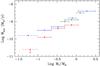 |
Fig. 11 Median values of Ṁacc as function of M∗. Red lines (with a central square) refer to σ Ori Class II and TD disks; the lowest mass bin should be considered as an upper limit only (see text). Blue lines (crosses) show the distribution for ρ-Oph (data from Natta et al. 2006, see Appendix A); green lines (circles) for Tr 37 (data from Sicilia-Aguilar et al. 2010). (A color version of this figure is available in the online journal.) |
6.2. Mass accretion rates vs disks morphologies
Figure 12 plots the mass accretion rates for the σ Ori sample as function of the excess over the photospheric emission for the four IRAC bands and for the 24 μm MIPS band. The excess emission is defined as the difference between the observed (Spitzer-I) color and that of Class III stars of the same effective temperature, assuming that no excess is present in the I band. In each panel, the horizontal bars show the median of the excess distribution for Class II disks and the lower and upper first quartile; for comparison, we also show the lower and upper first quartile of the excess for the Taurus median SED of classical disks (D’Alessio et al. 2006).
The median of the excess emission distributions is lower in σ Ori than in Taurus, as expected if on average σ Ori stars are older than Taurus objects, suggesting a higher degree of grain settling in older regions (e.g., Hernandez et al. 2007). Note that the σ Ori sample includes lower-mass objects than the Taurus one, and that disk models predict lower excess fluxes for BDs in this range of wavelengths; however, we do not find any correlation of the measured excess with the mass of the star, and we tend to exclude that the difference between the two regions is due to the different mass range only. The figure also shows the location of the 11 EV disks with a determination of Ṁacc and the 4 TD; for six of them we also show complete SEDs and Hα profiles in Appendix C.
There is no statistically significant correlation of Ṁacc with the excess emission. However, there are a few aspects of these plots that can be understood if, as expected in viscous models, Ṁacc traces the surface density of the inner disk. Objects with Ṁacc ~ 10-10−10-9 M⊙/y are distributed over the whole range of excess values. This is expected in optically thick disks, where the observed emission depends on inclination, inner radius and degree of flaring, but not on the actual disk surface density. Objects with Ṁacc ≲ 10-10 M⊙/y tend to have very low excess in all Spitzer bands. We think that most of them have in fact optically thin disks, which are characterized by much lower emission, roughly proportional to the surface density, i.e., to Ṁacc. The value Ṁacc ~ 10-10 M⊙/y is a reasonable threshold for the transition from optically thick to optically thin (inner) disks (D’Alessio et al. 2006).
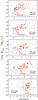 |
Fig. 12 Ṁacc vs. excess emission (in mag) in the four IRAC Spitzer bands and for the 24 μm MIPS band. The median excess emission and first quartiles are shown in each panel by the red (thick) horizontal lines; for comparison, we also plot the median Taurus class II SED (black (thin) line; D’Alessio et al. 2006). Symbols as in Fig. 7. (A color version of this figure is available in the online journal.) |
A last point to note is that disks with Ṁacc ≳ 10-9 M⊙/y have all large excess emission (in the upper quartile of the distribution), and indeed the upper envelope of the Ṁacc distribution seems to correlate with the amount of excess emission. Given the small number of objects in the high range of Ṁacc, the significance of this is unclear. If true, it would suggest a very interesting relation between Ṁacc and grain growth and settling, i.e., processes that can change the grain opacity and the disk flaring.
The potential of plots like Fig. 12 in constraining disk model parameters should be exploited further. However, this is well beyond the scope of this paper.
Figure 12 also shows the location of the 11 EV disks with an Ṁacc determination. Nine of them have upper limits to Ṁacc, some well below 10-10 M⊙/y, and very small excess emission, generally below the lower quartile of the Class II distribution. From the upper limits to Ṁacc, it is likely that at least half of them are indeed optically thin disks. There are two exceptions, one (SO908) is probably a missclassified Class II object, as it shows significant excess emission in all bands and broad Hα emission, consistent with its measured accretion rate (Ṁacc = 4 × 10⁻¹⁰ M⊙/y) (see Appendix C). The other EV object (SO1009) has one of the highest accretion rates in our sample (1.2 × 10⁻⁹ M⊙/y) and no detectable excess emission in all bands; indeed, its classification as a disk object is dubious. No additional data are available in the literature, and we may have detected a strong chromospheric flare. It would be interesting to monitor this object further.
The location of the four TD in Fig. 12 is also shown. They are scattered through the plot: two (SO818 and SO897) are consistent (both in Ṁacc and excess emission, see also Appendix C) with optically thick inner disks. One (SO1268) has very likely a very optically thin inner disk, with a very low upper limit to Ṁacc(~9 × 10-12 M⊙/y) and small excess emission even at 24 μm. The fourth TD object (SO299) has an accretion rate typical for its mass, 24 μm excess as Class II of similar accretion rate, but negligible excess in the IRAC bands. The large spread of properties of TD confirms the analysis of Muzerolle et al. (2010) and Sicilia-Aguilar et al. (2010) and their conclusions that very likely the “transitional” SEDs trace a variety of different physical situations.
7. Conclusions
We reported the results of a U-band survey with FORS1/VLT of a large area in the σ Ori star-forming region. We combined the U-band photometry with literature results to compute accretion luminosity and mass accretion rates from the U-band excess emission for all objects detected by Spitzer in the FORS1 field and classified by Hernandez et al. (2007) as likely members of the cluster. In total, there are 72 objects with evidence of a disk from near- and mid-IR photometry and 115 class III (diskless) stars. Among the disk objects, four (out of the seven identified by Hernandez et al. 2007) are transitional disks, and 14 are evolved disks. We derived the photospheric parameters of all stars from the existing V,R,I, and J photometry and used the U-λ colors of class III as templates for the photospheric and possible chromospheric emission. Our final sample, for which we provide estimates of the mass accretion rates, contains 58 Class II (49 class II stars for which we derive the accretion properties from the U-band excess emission, and nine stars with accretion properties from literature, for which we checked the consistency with our results), four TD and 11 EV disks, over a mass range of between ~0.06 and ~1.2 M⊙.
We analyzed the behavior of Ṁacc as function of mass and age of the individual stars, of the properties of the IR SED, and of the distance from the bright star σ Ori.
There is no correlation of Ṁacc with the distance from σ Ori, confirming that the effect of the O9.5 star on its surroundings is not strong (see also Hernandez et al. 2007); however, our sample does not include objects with projected distances smaller than 0.1 pc.
We find a strong relation between Ṁacc and M∗, with a very large spread of Ṁacc values for any given M∗, similar to other star-forming regions (Calvet et al. 2004; Natta et al. 2006; Fang et al. 2009; Sicilia-Aguilar et al. 2010). If fitted with a linear correlation, the slope is 1.6 ± 0.4. As noted by Vorobyov & Basu (2009) for a compilation of accretion rates in different star-forming regions, a linear fit is not the best description of the data. We computed median Ṁacc values and showed that the relation between Ṁacc and M∗ is flatter at higher masses and steepens significantly for very low-mass stars and BDs. Such a trend is predicted by models of core collapse and disk evolution that include viscosity and gravitational instabilities (Vorobyov & Basu 2009), which control the evolution of more massive disks.
These models follow the disk evolution to the age of σ Ori, under the assumption that disks evolve only by accreting onto the star. However, other processes such as photoevaporation and/or planet formation, may cause disk dissipation (e.g. Hollenbach 2000; Dullemond et al. 2009). This may be a selective effect, which affects higher mass stars more than lower mass stars, changing the observed dependence of the Ṁacc distribution with M∗. We have compared the Ṁacc-M∗ distribution in σ Ori to that of the two other star-forming regions in the literature for which an IR-selected sample is available, namely ρ-Oph (Natta et al. 2006 and Appendix A) and Tr 37 (Sicilia-Aguilar et al. 2010). The comparison indicates that the median Ṁacc values for higher M∗ are closer than predicted by simple viscous models, suggesting that selective disk dissipation may be important. However, we note that the significance of this comparison is not very strong, because the results for ρ-Oph are uncertain and the number of objects in each mass bin is not large. Moreover, the number and distribution of upper limits to Ṁacc affects the determination of median values in some mass ranges and prevents us from deriving upper and lower quartiles of the distributions.
The behavior of Ṁacc as function of the excess emission in the Spitzer bands suggests that at Ṁacc ~ 10-10 M⊙/y the (inner) disks change from optically thin to optically thick. Objects with Ṁacc in the range ~10-10−10-9M⊙/y span the whole range of observed excesses, from very low to very large. Objects with Ṁacc ≳ 10-9 M⊙/y (the largest values in the sample) all have large IR excess. Viscous disk models (e.g., D’Alessio et al. 2006) predict that for Ṁacc = 10-10 M⊙/y the surface density at 1 AU from a T Tauri star will be on the order of 1–10 g cm-2, depending on the grain properties and dust settling. The emission of these disks in the Spitzer bands will be optically thin, unless grains are sub-micron size. The trend we tentatively observe among optically thin and optically thin disks, which needs to be confirmed in larger samples, may indicate a link between the mass accretion rate and the grain properties, which in turn control the disk geometry,a connection that is worth to be further explored.
The four TD stars included in our sample seem to cover a variety of properties, and only one of them has a mass accretion rate as Class II of similar mass, and negligible excess emission to wavelengths >8 μm. The other three could not be distinguished from Class II objects in the Ṁacc vs. excess emission plots. We can only agree with the conclusions that the “transitional” properties of the SEDs are likely caused by a variety of different properties (Muzerolle et al. 2010; Sicilia-Aguilar et al. 2010).
Online material
Appendix A: ρ Ophiucus
The ρ-Oph sample is particularly interesting, because it is similar to the σ Ori one in being an IR-selected sample of class II, complete to a limiting mass of about 0.05 M⊙ (Bontemps et al. 2001). Natta et al. (2006) computed mass accretion rates from the luminosity of Paβ assuming a distance of 160 pc; since no extensive spectral type determinations were available, they followed the method outlined by Bontemps et al. (2001) and derived the stellar parameters assuming coeval star formation at 0.5 My and the evolutionary tracks of D’Antona & Mazzitelli (1998, the isochrone method). They found that the mass accretion rates could be fitted by a linear relation ∝ M ∗ 1.8 ± 0.2 over a mass interval 0.03–3 M⊙, with a very large spread for any given M∗. However, the Natta et al. (2006) results need to be reconsidered, since new measurements of the ρ-Oph distance yield considerably low values, 120–130 pc (Lombardi et al. 2008; Loinard et al. 2008; Snow et al. 2008). The corresponding decrease in luminosity implies an older age for the region. We have redetermined stellar parameters and mass accretion rates for all objects in Natta et al. (2006), adopting a distance of 130 pc and evolutionary tracks of Baraffe et al. (1998) for 1 My. The new values of Ṁacc are somewhat lower than previous ones, and M∗ higher, especially for higher masses (see Fig. A.1).
As a consequence, if fitted with a single power-law, the correlation between Ṁacc and M∗ is flatter, with a slope of 1.3 ± 0.2. The new distance, the older age and the different evolutionary tracks contribute to this result. In particular, the dependence of the Ṁacc – M∗ relation on the adopted evolutionary tracks is well known (see Fang et al. 2009) and is particularly strong in ρ-Oph, given the method used to determine the stellar parameters.
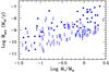 |
Fig. A.1 Mass accretion rate versus stellar masses for the star of the ρ-Oph sample. The stellar parameters and the accretion properties were recalculated assuming a distance of 130 pc (Lombardi et al. 2008) instead of 160 pc assumed by Natta et al. (2006), and 1 My age. |
Appendix B: BD and very low-mass stars from the Lodieu et al. photometric survey
An independent sample of very low-mass stars and brown dwarfs has been selected from the list of σ Ori members and candidate members of Lodieu et al. (2009). We applied a first selection criterium on the z,(z − J) diagram computed Teff by comparing observed z,Y,J colors to synthetic ones from the theoretical models of Baraffe et al. (1998) for log g = 4.0 and luminosities from the observed J mag and model-predicted bolometric corrections. We then performed a further selection based on the location of the objects on the HR diagram, excluding all stars with M∗ > 0.13 M⊙. Our sample of candidate young very low-mass stars and BDs in σ Ori is then formed by 80 objects, 40 of which were included in the U-band FORS1 survey.
Spitzer IRAC detections exist for 21/40 objects; three of them are uncertain members according to Hernandez et al. (2007). Of the 21, six are classified as class II, one is a transitional disk, one an evolved disk and 13 are class III objects. The 18 confirmed members are included in the sample analyzed in the main text of the paper. Note that the determination of the stellar parameters, Teff in particular is performed using different photometric bands with respect to the bands used in the main text; the difference in Teff are in general within the uncertainties discussed in Sect. 3.1; however, some of the objects in Table 2, although included in the Lodieu sample, were not selected with the criteria applied here.
Of the 40 objects in our sample, 20 have been detected in the U-band, while for the other 20 we have upper limits only. We derived the accretion luminosity and mass accretion rates as in Sect. 4.3. The calibration of the photospheric colors (U − J) and (U − I) as function of Teff using our U-band photometry of Class III objects extends to Teff ~ 2900 K (Sect. 4.1); we compare it to synthetic colors from the Baraffe et al. (1998) model atmosphere to extend the relations to lower Teff. The Class III colors agree well with the models; the results are shown in Fig. B.1.
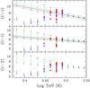 |
Fig. B.1 U-λ colors as function of Teff. The red circles are objects with measured U-band fluxes, arrows are objects with U-band upper limits. The squares are model-predicted colors for different gravity, from 5.5 (black squares, top) to 3.5 (blue squares, lowest). The solid lines show the best-fit relations for Class III derived in Sect. 4.1, extrapolated to lower Teff; dashed lines are ± 2σ. We will consider as accretors objects with colors below the photospheric strip: five BDs have clear evidence of U-band excess (note that for two we only have two colors), one only marginal evidence (from (U − I) and (U − J), while (U − Z) is photospheric). Hereafter we mark the upper limit as dashes for clarity. (A color version of this figure is available in the online journal.) |
Figure B.2 shows Ṁacc vs. M∗; we find that only five objects (all with M∗0.06 M⊙) have Ṁacc > −10.8, the median in Sect. 6.1. of these, two are class II sources (SO500 and SO848, also in Table 2), one is a class III (SO641, possibly misclassified), three have no Spitzer detections. No other object with higher values of Ṁacc is detected.
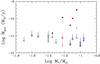 |
Fig. B.2 Mass accretion rate as function of M∗. Dots are class II objects with measured Ṁacc, the cross is a class III stars with measured Ṁacc, and diamonds refer to object with no Spitzer data. Arrows are objects with upper limits (both U-band detections and non-detections). Colors (only in the on-line version) indicate the SED Class : red for class II, blue for class III; black for objects with no Spitzer data. (A color version of this figure is available in the online journal.) |
Appendix C: SEDs and Hα of EV and TD objects
In this section, we show SEDs (Fig. C.1) and Hα profiles (Fig. C.2) of a subset of two TD and four EV stars observed with SARG@TNG (Sect. 2.4) and Giraffe (Sacco et al. 2008). A summary of the Hα properties is given in Table C.1, where 10% Hα represents the width of Hα at 10% of the line’s peak intensity, and pEW is the pseudo-equivalent width. Below we will briefly comment on each object.
SO587. This EV disk was extensively studied by Rigliaco et al. (2009). It exhibits modest excess emission (well below the lower quartiles of the distributions) in the IRAC bands and at 24 μm. It shows a symmetric and narrow Hα emission profile with the peak close to the line center (type I profile following the classification of Reipurth et al. (1996)). Based on the available U-band photometry (Wolk 1996), the narrow Hα and the strength and profiles of the [S ii] and [N ii] forbidden lines, Rigliaco et al. (2009) suggested that the disk was being photoevaporated and that the forbidden lines were coming from the photoevaporation flow, possibly driven and certainly illuminated by the star σ Ori. A crucial ingredient of this model was the high ratio between the mass-loss and the mass-accretion rate. Our results confirm this interpretation. Although relatively bright in U, the object does not have a measurable U-band excess (i.e., it lies inside the photospheric strip of Fig. 4) and we estimate an upper limit to log Ṁacc of −9.45 M⊙/y, consistent with the value −9.52 M⊙/y derived in Rigliaco et al. (2009).
SO615. This is a relatively massive, luminous star. Its SED is typical of a flat disk up to 24 μm. We cannot measure Ṁacc from the U-band, which is already saturated by the photospheric emission alone, but we can estimate a value of log Ṁacc = −8.25 M⊙/y from the U = 15.96 mag measurement of Wolk (1996). The Hα has a complex profile, with broad wings, deep redshifted and blueshifted absorption and a narrow, slightly redshifted emission in the center. Similar profiles are observed for higher numbers of the Balmer series (“YY Orionis like profiles”; Walker 1972) and are associated with extensive infall and outflow rates, consistent with the very high value of Ṁacc. Unfortunately, the SARG SO615 spectrum is rather noisy.
SO759. Classified as EV disk star by Hernandez et al. (2007). The SED has negligible excess up to 8 μm, but a significant one at 24 μm, not very different from the SED of some TD objects. The Hα is rather narrow and symmetric, with a moderate red/blue asymmetry (type I profile, Reipurt et al. 1996). The 10% Hα width of 157 ± 12 km s-1 and the upper limit log Ṁacc < −9.67 M⊙/y is not stringent for an object of 0.3 M⊙, but, combined with the Hα properties, it suggests that this is a low accretor (if any).
SO818. Classified as TD. This star shows significant excess emission, in the higher quartile at 3.6, 4.5, 5.8 and at 24 μm. We measure Ṁacc= −9.45 M⊙/y, typical of optically thick disks. The Hα is broad (10% width of 332 ± 25 km s-1) and shows an inverse P-Cygni profile, with the emission peak at the line center position. The red-shifted absorption goes below the continuum (type IVR), confirming the evidence of a high accretion rate.
SO897. Classified as TD; the IRAC excess emission is clearly detected, but lower than the σ Ori medians, while the 24 μm excess is strong. We measure a lower limit to Ṁacc(>−9.13 M⊙/y), but the star is clearly accreting. We have two measurements of the Hα profile, one with Giraffe in October 2004 and one with SARG acquired in January 2009. Within these two epochs the maxima change in position and strength, with the primary one blue-shifted in 2004 and red-shifted in 2009, and the secondary one with opposite behaviour. The wavelength separation of the blue and red emission peaks decreases from 2004 and 2009, while the central reversal seems to be at the line center in the first epoch and then slightly blue-shifted in the second epoch. The profile changes from IIR to IIB, following the Reipurt et al. (1996) scheme, where these types are characterized by secondary peaks exceeding half the strength of the primary peaks, as we observe. This is a common phenomenon in accreting T Tauri stars, probably due to the interplay of variable accretion and mass-loss.
SO908. EV disk, with excess emission within the lower quartiles at all IRAC wavelengths, and significant excess at 24 μm. We measure Ṁacc = –9.37 M⊙/y, typical of optically thick disks. The Hα is broad and asymmetric, with less emission in the red than in the blue. This type of profile (IIIR) is the less frequent in the scheme classification of Reipurt et al. (1996). Following the radiative transfer models developed by Kurosawa et al. (2006), this profile morphology requires some obscuration by the dusty disk, i.e. a high inclination, explaining the rarity of the profile. A highly inclined disk is consistent with the SED properties.
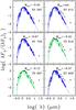 |
Fig. C.1 SEDs of four EV disks and 2 TD. The squares shows the observed fluxes (see Table C.2). The lines plot the model atmosphere from Allard et al. (2000) at the appropriate Teff, log g = 4.0, normalized to the J band. Each panel gives the name of the star (see Table C.1) and the mass accretion rate. |
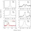 |
Fig. C.2 Hα line profiles of six stars of the sample normalized to the continuum. The spectra have been obtained either in 2004 with FLAMES/Giraffe by Sacco et al., with a spectral resolution R = 17000, or by Rigliaco et al., in 2009 with SARG, with a spectral resolution R = 29000, as indicated in Table C.1. |
U-band and collected literature photometry. The U-band magnitudes have been obtained with FORS1@VLT, the optical photometry is from Sherry et al. (2004), Kenyon et al. (2005), Zapatero-Osorio et al. (2002), Béjar et al. (2001) and Wolk (1996). JHK magnitudes are from the Two Micron All Sky Survey (2MASS) (Cutri et al. 2003). The magnitudes in the four channels of the Infrared Array Camera (IRAC; 3.8–8.0 μm) and the first channel of the Multiband Imaging Photometer for Spitzer (MIPS; 24 μm) are from Hernandez et al. (2007).
iraf is distributed by National Optical Astronomy Observatories, which are operated by the Association of Universities for Research in Astronomy, Inc., under cooperative agreement with the National Science Foundation.
Acknowledgments
We thank Fabrizio Massi for useful suggestions on the data reduction and Nicolas Lodieu for providing the data on the σ Ori brown dwarfs. This publication is based on observations made with FORS1@VLT and SARG@TNG. We acknowledge the staff of the ESO Data Management and Operations department, who performed our observations in service mode.
References
- Béjar, V. J. S., Zapatero-Osorio M. R., & Rebolo R. 1999, ApJ, 521, 671 [NASA ADS] [CrossRef] [Google Scholar]
- Béjar, V. J. S., Martin, E. L., Zapatero Osorio, M. R., et al. 2001, ApJ, 556, 830 [NASA ADS] [CrossRef] [Google Scholar]
- Baraffe, I., Chabrier, G., Allard, F., & Hauschildt, P. H. 1998, A&A 337, 403 [Google Scholar]
- Bontemps, S., André, P., Kaas, A. A., et al. 2001, A&A, 372, 173 [NASA ADS] [CrossRef] [EDP Sciences] [Google Scholar]
- Briceño, C., Vivas, A. K., Calvet, N., et al. 2001, Science, 291, 93 [NASA ADS] [CrossRef] [Google Scholar]
- Brown, A. G. A., de Geus E. J., & de Zeeuw P. T. 1994, A&A, 289, 101 [NASA ADS] [Google Scholar]
- Caballero, J. A. 2007, A&A 466, 917 [Google Scholar]
- Caballero J. A.,Béjar, V.J.S., Rebolo, R., et al. 2007, A&A, 470, 903 [NASA ADS] [CrossRef] [EDP Sciences] [Google Scholar]
- Calvet, N., D’Alessio, P., Hartmann, L., et al. 2002, ApJ, 568, 1008 [NASA ADS] [CrossRef] [Google Scholar]
- Calvet, N., Muzerolle, J., Briceno, C., et al. 2004, AJ, 128, 1294 [NASA ADS] [CrossRef] [Google Scholar]
- Calvet, N., D’Alessio, P., & Watson, D. M. 2005, ApJ 630, L185 [NASA ADS] [CrossRef] [Google Scholar]
- Clarke, C. J. 2007, 376, 1350 [Google Scholar]
- Currie, T., Lada, C., Plavchan, P., et al. 2009, ApJ 698, 1 [NASA ADS] [CrossRef] [Google Scholar]
- Cutri, R. M., Skrutskie, M. F., van Dyk, S., et al. 2003, 2MASS All Sky Catalog of Point Sources, The IRSA 2MASS All-Sky Point Source Catalog, NASA/IPAC Infrared Science Archive (Pasadena, CA: NASA/IPAC), http://irsa.ipac.caltech.edu/application/Gator [Google Scholar]
- D’Alessio, P., Calvet, N., Hartmann, L., et al. 2006, ApJ, 638, 314 [NASA ADS] [CrossRef] [Google Scholar]
- Dullemond, C., Natta, A., & Testi, L. 2006, ApJ, 645, L69 [NASA ADS] [CrossRef] [Google Scholar]
- Dullemond, C. P., Hollenbach, D., Kamp, I., & D’Alessio, P. 2007, Protostars and Planets V, ed. B. Reipurth, D. Jewitt, & K. Keil (Tucson, AZ: Univ. Arizona Press), 783 [Google Scholar]
- Fang, M., van Boekel, R., Wang, W., et al. 2009, A&A, 504, 461 [NASA ADS] [CrossRef] [EDP Sciences] [Google Scholar]
- Feigelson, E. D., & Nelson, P. I. 1985, ApJ, 293, 192 [NASA ADS] [CrossRef] [Google Scholar]
- Franciosini, E., Pallavicini, R., & Sanz-Forcada, J. 2006, A&A, 446, 501 [NASA ADS] [CrossRef] [EDP Sciences] [Google Scholar]
- Gomez de Castro, A. I., Franqueira, M., Huelamo, N., & Verdugo, E. 1998, Ap&SS, 261, 129 [NASA ADS] [CrossRef] [Google Scholar]
- Gorti, U., & Hollenbach, D. 2009, ApJ, 690, 1539 [Google Scholar]
- Gullbring, E., Hartmann, L., Briceño, C., & Calvet N. 1998, ApJ, 492, 323 [NASA ADS] [CrossRef] [Google Scholar]
- Jeffries, R. D., Maxted, P. F. L., Oliveira, J. M., & Naylor, T. 2006, MNRAS, 371, L10 [Google Scholar]
- Hartigan, P., Kenyon, S. J., Hartmann, L., et al. 1991, ApJ, 382, 617 [NASA ADS] [CrossRef] [Google Scholar]
- Hartmann, L., Calvet, N., Gullbring, E., & D’Alessio, P. 1998, ApJ, 495, 385 [NASA ADS] [CrossRef] [Google Scholar]
- Hartmann, L., Megeath, S. T., Allen, L., et al. 2005, ApJ, 629, 881 [NASA ADS] [CrossRef] [Google Scholar]
- Hartmann, L., Calvet, N., Gullbring, E., & D’Alessio, P. 2006, ApJ, 648, 484 [NASA ADS] [CrossRef] [Google Scholar]
- Herczeg, G., & Hillenbrand, L. A. 2008, ApJ, 681, 594 [NASA ADS] [CrossRef] [Google Scholar]
- Hernández, J., Hartmann, L., Megeath, S. T., et al. 2007, ApJ, 662, 1067 [NASA ADS] [CrossRef] [Google Scholar]
- Hillenbrand, L. A. 2009, IAUS, 258, 81 [Google Scholar]
- Hollenbach, D., Yorke, H., & Johnstone, D. 2000, Protostars and Planets IV, ed. V. Mannings, A. P. Boss, & S. S. Russell (Tucson, AZ: Univ. Arizona Press), 401 [Google Scholar]
- Kenyon, S. J., & Hartmann, L. 1995, ApJS, 101, 117 [NASA ADS] [CrossRef] [Google Scholar]
- Kenyon, M. J., Jeffries, R. D., Naylor, T., et al. 2005, 356, 89 [Google Scholar]
- Kurosawa, R., Harries, T. J., & Symington, N. H. 2006, MNRAS, 372, 1879 [NASA ADS] [CrossRef] [Google Scholar]
- Landolt, A. U. 1992, AJ, 104, 340 [NASA ADS] [CrossRef] [Google Scholar]
- Lodieu, N., Zapatero Osorio, M. R., Rebolo, R., et al. 2009, A&A, 505 1115 [NASA ADS] [CrossRef] [EDP Sciences] [Google Scholar]
- Loinard, L., Torres, R. M., Mioduszewski, A. J., & Rodrguez, L. F. 2008, IAU Symp., 248, 186 [NASA ADS] [Google Scholar]
- Lombardi, M., Lada, C. J., & Alves, J. 2008, A&A, 480, 785 [NASA ADS] [CrossRef] [EDP Sciences] [Google Scholar]
- Luhman, K. L., Stauffer, J. R., Muench, A. A., et al. 2003, ApJ, 593, 1093 [NASA ADS] [CrossRef] [Google Scholar]
- Muzerolle, J., Hillenbrand, L., Calvet, N., et al. 2003, ApJ, 592, 266 [NASA ADS] [CrossRef] [Google Scholar]
- Muzerolle, J., Allen, L., Megeath, T., et al. 2010, ApJ, 708, 1107 [NASA ADS] [CrossRef] [Google Scholar]
- Natta, A., Testi, L., Muzerolle, J., et al. 2004, A&A, 424, 603 [NASA ADS] [CrossRef] [EDP Sciences] [Google Scholar]
- Natta, A., Testi, L., & Randich, S. 2006, A&A, 452, 245 [NASA ADS] [CrossRef] [EDP Sciences] [Google Scholar]
- Oliveira, J. M., Jeffries, R. D., & van Loon, J. T. 2004, MNRAS, 347, 1327 [NASA ADS] [CrossRef] [Google Scholar]
- Oliveira, J. M., Jeffries, R. D., van Loon, J. T., et al. 2006, MNRAS, 369, 272 [NASA ADS] [CrossRef] [Google Scholar]
- Perryman, M. A. C., Lindegren, L., Kovalevsky, J., et al. 1997, A&A, 323, L49 [NASA ADS] [Google Scholar]
- Persson, S. E., Murphy, D. C., Krzeminski, et al. 1998, AJ, 116, 2475 [NASA ADS] [CrossRef] [Google Scholar]
- Rigliaco, E., Natta, A., Randich, S., & Sacco, G. 2009, A&A, 495, L13 [NASA ADS] [CrossRef] [EDP Sciences] [Google Scholar]
- Reipurth, B., Pedrosa, A., & Lago, M. T. V. 1996, A&ASS, 120, 229 [NASA ADS] [CrossRef] [EDP Sciences] [Google Scholar]
- Sacco, G., Franciosini, E., Randich, S., & Pallavicini, R. 2008, A&A, 488, 167 [NASA ADS] [CrossRef] [EDP Sciences] [Google Scholar]
- Sherry, W. H., Walter, F. M., & Wolk, S. J. 2004, AJ, 128, 2316 [NASA ADS] [CrossRef] [Google Scholar]
- Sicilia-Aguilar, A., Hartmann, L., Szentgyorgyi, A., et al. 2005a, AJ, 129, 363 [NASA ADS] [CrossRef] [Google Scholar]
- Sicilia-Aguilar, A., Hartmann, L., Hernández, J., et al. 2005b, AJ, 130, 188 [NASA ADS] [CrossRef] [Google Scholar]
- Sicilia-Aguilar, A., Henning, Th., & Hartmann, L. 2010, AJ, 710, 597 [NASA ADS] [CrossRef] [Google Scholar]
- Snow, T. P., Destree, J. D., & Welty, D. E. 2008, ApJ, 679, 512 [NASA ADS] [CrossRef] [Google Scholar]
- Vorobyov, E. I., & Basu, S. 2008, ApJ, 676, 139 [Google Scholar]
- Vorobyov, E. I., & Basu, S. 2009, MNRAS, 393, 822 [NASA ADS] [CrossRef] [Google Scholar]
- Walker, M. 1972, ApJ, 175, 89 [NASA ADS] [CrossRef] [Google Scholar]
- Wolk, S. J. 1996, Ph.D. Thesis [Google Scholar]
- ZapateroOsorio, M. R., Béjar, V. J. S., Pavlenko, Y., et al. 2002, A&A, 384, 937 [NASA ADS] [CrossRef] [EDP Sciences] [Google Scholar]
All Tables
Accretion properties of the class II objects and objects with transitional and evolved disks.
U-band and collected literature photometry. The U-band magnitudes have been obtained with FORS1@VLT, the optical photometry is from Sherry et al. (2004), Kenyon et al. (2005), Zapatero-Osorio et al. (2002), Béjar et al. (2001) and Wolk (1996). JHK magnitudes are from the Two Micron All Sky Survey (2MASS) (Cutri et al. 2003). The magnitudes in the four channels of the Infrared Array Camera (IRAC; 3.8–8.0 μm) and the first channel of the Multiband Imaging Photometer for Spitzer (MIPS; 24 μm) are from Hernandez et al. (2007).
All Figures
|
Fig. 1 Fields in the σ Ori cluster that have been imaged with FORS1 (solid boxes). Crosses (blue) show class III stars, circles (red) class II, TD and EV object, as classified by Hernandez et al. (2007). |
| In the text | |
|
Fig. 2 U-band magnitude from Wolk (1966) and this work. Dashed lines correspond to an interval of ± 0.5 mag. |
| In the text | |
|
Fig. 3 Location of the observed objects (class III, class II, and objects with “non-classical” disks, as labeled) on the HR diagram. Evolutionary tracks and isochrones are taken from Baraffe et al. (1998). Stellar masses and ages are labeled. The horizontal bar refers to the error on the effective temperature, the vertical bar reflects the error of the bolometric correction of the ZAMS stars related to the error on the effective temperatures. |
| In the text | |
|
Fig. 4 Colors of Class III stars vs. effective temperature. Blue horizontal lines plot (U − J), red crosses (U − I), green 45 deg lines (U − R), cyan –45 deg lines (U − V), as labeled. The solid lines show the best fit, the dashed lines ± 2σ. In the text, we will define the region between the dashed lines as the photospheric strip. (A color version of this figure is available in the online journal.) |
| In the text | |
|
Fig. 5 Values of the accretion luminosity derived from (U − J), (U − R), (U − V) vs. the value derived from (U − I), as described in the text for a sub-sample of 30 objects. The dashed lines correspond to ± 0.5 in log Lacc. |
| In the text | |
|
Fig. 6 Comparison between Lacc computed from Paγ (Gatti et al. 2008) and Lacc obtained from U-band photometry for stars in common. The dashed line refers to the same value of Lacc, the dashed-dotted lines to ± 0.5 in log Lacc. |
| In the text | |
|
Fig. 7 Accretion luminosity as a function of the stellar luminosity for class II, EV, and TD disks, as labeled. The dashed lines show Lacc/Lstar = 0.001, 0.01, and 0.1, respectively. The crosses surronded by a circle are the class II stars included here from the Gatti et al. (2008) sample, and listed in Table 3. Different colors for lower and upper limits can be distinguished in the online version of the journal. |
| In the text | |
|
Fig. 8 Mass accretion rate as function of stellar mass. Symbols as in Fig. 7. (A color version of this figure is available in the online journal.). |
| In the text | |
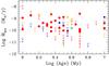 |
Fig. 9 Mass accretion rate as function of the age of the stars. Symbols as in Fig. 7. |
| In the text | |
|
Fig. 10 Mass accretion rates versus projected distance from the bright stars σ Ori in parsec. (A color version of this figure is available in the online journal.) |
| In the text | |
|
Fig. 11 Median values of Ṁacc as function of M∗. Red lines (with a central square) refer to σ Ori Class II and TD disks; the lowest mass bin should be considered as an upper limit only (see text). Blue lines (crosses) show the distribution for ρ-Oph (data from Natta et al. 2006, see Appendix A); green lines (circles) for Tr 37 (data from Sicilia-Aguilar et al. 2010). (A color version of this figure is available in the online journal.) |
| In the text | |
|
Fig. 12 Ṁacc vs. excess emission (in mag) in the four IRAC Spitzer bands and for the 24 μm MIPS band. The median excess emission and first quartiles are shown in each panel by the red (thick) horizontal lines; for comparison, we also plot the median Taurus class II SED (black (thin) line; D’Alessio et al. 2006). Symbols as in Fig. 7. (A color version of this figure is available in the online journal.) |
| In the text | |
|
Fig. A.1 Mass accretion rate versus stellar masses for the star of the ρ-Oph sample. The stellar parameters and the accretion properties were recalculated assuming a distance of 130 pc (Lombardi et al. 2008) instead of 160 pc assumed by Natta et al. (2006), and 1 My age. |
| In the text | |
|
Fig. B.1 U-λ colors as function of Teff. The red circles are objects with measured U-band fluxes, arrows are objects with U-band upper limits. The squares are model-predicted colors for different gravity, from 5.5 (black squares, top) to 3.5 (blue squares, lowest). The solid lines show the best-fit relations for Class III derived in Sect. 4.1, extrapolated to lower Teff; dashed lines are ± 2σ. We will consider as accretors objects with colors below the photospheric strip: five BDs have clear evidence of U-band excess (note that for two we only have two colors), one only marginal evidence (from (U − I) and (U − J), while (U − Z) is photospheric). Hereafter we mark the upper limit as dashes for clarity. (A color version of this figure is available in the online journal.) |
| In the text | |
|
Fig. B.2 Mass accretion rate as function of M∗. Dots are class II objects with measured Ṁacc, the cross is a class III stars with measured Ṁacc, and diamonds refer to object with no Spitzer data. Arrows are objects with upper limits (both U-band detections and non-detections). Colors (only in the on-line version) indicate the SED Class : red for class II, blue for class III; black for objects with no Spitzer data. (A color version of this figure is available in the online journal.) |
| In the text | |
|
Fig. C.1 SEDs of four EV disks and 2 TD. The squares shows the observed fluxes (see Table C.2). The lines plot the model atmosphere from Allard et al. (2000) at the appropriate Teff, log g = 4.0, normalized to the J band. Each panel gives the name of the star (see Table C.1) and the mass accretion rate. |
| In the text | |
|
Fig. C.2 Hα line profiles of six stars of the sample normalized to the continuum. The spectra have been obtained either in 2004 with FLAMES/Giraffe by Sacco et al., with a spectral resolution R = 17000, or by Rigliaco et al., in 2009 with SARG, with a spectral resolution R = 29000, as indicated in Table C.1. |
| In the text | |
Current usage metrics show cumulative count of Article Views (full-text article views including HTML views, PDF and ePub downloads, according to the available data) and Abstracts Views on Vision4Press platform.
Data correspond to usage on the plateform after 2015. The current usage metrics is available 48-96 hours after online publication and is updated daily on week days.
Initial download of the metrics may take a while.