| Issue |
A&A
Volume 525, January 2011
|
|
|---|---|---|
| Article Number | A9 | |
| Number of page(s) | 7 | |
| Section | Interstellar and circumstellar matter | |
| DOI | https://doi.org/10.1051/0004-6361/200810611 | |
| Published online | 26 November 2010 | |
Spectroscopic [C i] mapping of the infrared dark cloud G48.65-0.29
1
I. Physikalisches Institut der Universität zu Köln,
Zülpicher Straße 77,
50937
Köln, Germany
e-mail: ossk@ph1.uni-koeln.de
2
SRON Netherlands Institute for Space Research,
PO Box 800, 9700 AV
Groningen, The
Netherlands
3
Kapteyn Astronomical Institute, University of
Groningen, PO Box
800, 9700 AV
Groningen, The
Netherlands
4
Max-Planck-Institut für Astronomie, Königstuhl 17, 69117
Heidelberg,
Germany
Received: 15 July 2008
Accepted: 7 October 2010
Aims. We report the first spectroscopic mapping of an atomic carbon line in an infrared dark cloud (IRDC). By observing the spatial distribution of the [C i] emission in an IRDC, comparing it with the 13CO emission and the known distribution of internal heating sources, we can quantify the role of internal and external UV irradiation in the production of atomic carbon.
Methods. We used the 2 × 4 pixel SMART receiver of the KOSMA observatory
on Gornergrat to map the [C i]  line in the IRDC G48.65-0.29 and compared
the resulting spectra with data from the BU-FCRAO 13CO 1–0 Galactic Ring
Survey.
line in the IRDC G48.65-0.29 and compared
the resulting spectra with data from the BU-FCRAO 13CO 1–0 Galactic Ring
Survey.
Results. The [C i]/13CO effective beam temperature ratio falls at about 0.3 with local deviations by less than a factor two. All velocity components seen in 13CO are also detected in [C i]. We find, however, significant differences in the morphology of the brightest regions seen in the two tracers. While 13CO basically follows the column density distribution derived from the near-infrared (NIR) extinction and the submm continuum, the [C i] emission peaks at the locations of the two known NIR point sources. We find C i/CO abundance ratios between 0.07 and 0.13 matching the lower end of the range previously measured in star-forming regions.
Conclusions. Evaluating the relative importance of the irradiation by embedded sources and by the Galactic interstellar UV field, we find that in G48.65-0.29 most [C i] emission can be attributed to externally illuminated surfaces. Embedded sources have a significant impact on the overall abundance distribution of atomic carbon as soon as they are found in an evolved state with noticeable NIR flux.
Key words: ISM: clouds / ISM: structure / ISM: abundances / ISM: individual objects: G48.65-0.29 / dust, extinction / ISM: atoms
© ESO, 2010
1. Introduction
Chemical models of interstellar gas predict that atomic carbon, Ci, occurs only in a transitional layer characterised by a moderate UV field which allows ionised carbon to recombine, but still leads to the dissociation of CO (Le Bourlot 1993; Oka et al. 2004; Röllig et al. 2006). In the picture of a simple cloud geometry with a well-defined interior and exterior of a cloud, [C i] is thus supposed to trace surfaces of molecular clouds exposed to UV radiation either from the external interstellar radiation field or from embedded stars (Ossenkopf et al. 2007). Its abundance and emission is modelled in the framework of photon-dominated regions (PDRs). Molecular cloud observations show, however, that their structure is rather described by a fractal distribution, where UV radiation can deeply penetrate and surfaces are found throughout the whole cloud (Falgarone et al. 2004), leading to a strong correlation in the distribution of atomic carbon and molecular tracers.
Bright [C i] emission has been observed towards several star-forming regions (e.g., Plume et al. 2000; Sun et al. 2008), where the intense UV radiation from young stars creates many PDRs throughout the clumpy ambient molecular clouds. To understand the origin of the [C i] emission and the Galactic abundance distribution of atomic carbon it is, however, essential to distinguish the mutual importance of PDRs within molecular clouds, created by star formation, and the PDRs at their outer surfaces produced by the interstellar radiation field illuminating them (Draine & Bertoldi 1996). Pineda & Bensch (2007) detected [C i] towards B68, only seeing the standard interstellar radiation field, but didn’t find a PDR model that fitted all of the observed lines.
To help resolving the question on the relative importance of inner and outer PDRs for the production of atomic carbon we decided to map the [C i] emission from an infrared dark cloud (IRDC), a site of potentially massive star formation in a very early stage (Rathborne et al. 2006; Simon et al. 2006). IRDCs were detected as dark patches in front of the bright diffuse IR emission from the Milky Way mapped by ISO and the MSX satellite (Pérault et al. 1996; Egan et al. 1998). Their column densities exceed 1023 cm-2, producing the strong dust absorption that led to their discovery. IRDC masses range from 103 to 104M⊙, the gas is typically cold (T < 25 K) and dense (n > 105 cm-3, Simon et al. 2006). Recent follow-up observations have revealed signs of active star (cluster) formation in numerous IRDCs (Rathborne et al. 2006, 2007).
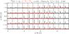 |
Fig. 1 Line profiles measured on 13CO 1–0 (black, BU-FCRAO Galactic Ring Survey)
and in [C i] |
We have observed the IRDC G48.65-0.29 (Simon et al. 2006), a cloud at a distance of 2.5 kpc in the direction towards W51, that was previously studied in several molecular transitions by Shipman et al. (2003), in the 450 μm and 850 μm continuum by Ormel et al. (2005), and in the mid-infrared (MIR), using the Spitzer Space Telescope, by Kraemer et al. (proposal 3121, see Van der Wiel & Shipman 2008). These observations have revealed several submm condensations and IR point sources indicating deeply embedded protostars.
This configuration is an ideal test bed to distinguish the role of internal and external UV fields for the distribution of atomic carbon, because the protostars are still too deeply embedded to allow their UV radiation to illuminate remote parts of the cloud. We find a clear distinction between inner and outer surfaces. By observing the spatial distribution of the [C i] emission and correlating this with the distribution of molecular material on the one hand and with the distribution of young stars within the IRDC on the other hand, we can discriminate between the effects of internal and external radiation for the formation of atomic carbon.
In Sect. 2 we describe the observations and the supplementary data used in the analysis. Section 3 summarises the results and in Sect. 4, we derive abundance ratios for a comparison with reference data and give a first interpretation of the results. Section 5 summarises the conclusions of the paper.
2. Observations
We have used the Sub-Millimeter Array Receiver for Two frequencies (SMART, Graf et al. 2003) at the Kölner Observatorium für
Sub-Millimeter Astronomie (KOSMA, Winnewisser et al.
1986) 3 m telescope on Gornergrat, Switzerland, to observe the G48 IRDC in the
492 GHz [C i] line. The observations were taken in March
2004 and February 2005. At that time, the SMART receiver was equipped with 4 pixels for the
460–490 GHz atmospheric window and 4 pixels for the 810 GHz window. The double sideband
system temperature at 492 GHz was about 250 K for three of the pixels, the fourth pixel was
under-pumped, so that we ignore all data from that pixel here.
We have mapped the cloud in a double beam-switch (DBS) raster mode using a chopper throw of 6 arcmin. Although the [C i] emission is in general extended, we can exclude any significant self-chopping effects due to the spatial and velocity structure of the IRDC as shown in the Appendix. The HPBW of the KOSMA telescope at 492 GHz is 55′′ and the main beam efficiency ηmb = 62%. The pointing accuracy of the telescope is better than 10′′, we typically measured a 1σ pointing scatter of about 3′′ in pointing checks at various sources. The SMART pixel separation is 115′′ and we have added in the mapping two telescope pointings to fill the pixel spacing so that we obtained a slightly undersampled map with a spacing of 38′′.
The IF signal was analysed with 4 × 1 GHz acousto-optical spectrometers with a spectral
resolution of 1.5 MHz, corresponding to a velocity resolution of 0.91 km s-1 at
492 GHz. The channel spacing is 1.04 MHz, corresponding to 0.63 km s-1. The
high-frequency channel of SMART was tuned to the upper (809 GHz)
[C i] line, but due to the higher receiver noise
(Tsys(DSB) ≈ 650 K) and the lower
atmospheric transparency at that frequency this provided only an upper limit of about 5 K
for the upper [C i] line.
line, but due to the higher receiver noise
(Tsys(DSB) ≈ 650 K) and the lower
atmospheric transparency at that frequency this provided only an upper limit of about 5 K
for the upper [C i] line.
For the analysis, we compare the new [C i] data data with the 13CO 1–0 maps taken in the Boston University – Five College Radio Astronomy Observatory (BU-FCRAO) Galactic Ring Survey (Jackson et al. 2006). They are given at a velocity resolution of 0.21 km s-1. While regridding the FCRAO data from Galactic to equatorial coordinates, in which the [C i] map was taken, the data were resampled to the same spatial resolution of 55′′. We provide all spectra on the original antenna temperature scale.
As both [C i] and 13CO show emission extending beyond the main beams of the telescopes, the measured intensity is given by the superposition of the main beam detection and some error beam pickup. In the Appendix we have estimated the effective beam efficiencies for this configuration using the known main and error beam efficiencies and the approximate configuration of the IRDC. To convert the antenna temperature to this effective beam temperature scale, the KOSMA data have to be divided by an effective beam efficiency of 0.69 and the FCRAO data by 0.70. Since these numbers are almost identical, all ratios are unaffected by the beam coupling, so that they have the same value when taken on the antenna temperature or the effective beam temperature scale.
3. Results
Figure 1 shows all measured [C i] spectra on top of the corresponding FCRAO 13CO 1–0 spectra covering the G48 IRDC. We find the same spectral features in 13CO and [C i]. There are four dominant velocity components, at 34 km s-1, 40 km s-1, 52 km s-1, and 57–59 km s-1, but also some emission at intermediate velocities between the components at 34 and 40 km s-1 and the components at 52 and 58 km s-1, indicating bridges of gas between the components. Within the noise limits we find no significant differences in the spectral shapes of the [C i] and 13CO 1–0 lines. Simon et al. (2006) identified the 34 km s-1 component with the IRDC based on the morphological similarity of the 13CO component and the mid-IR dark cloud in the MSX image. The 52 km s-1 component has a kinematic distance of more than 4 kpc representing a separate cloud which appears accidentally in the same line-of-sight but is unrelated to the IRDC.
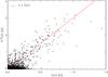 |
Fig. 2 Scatter plot of the measured 13CO and [C i] intensities for different channels and points across the cloud. The red line indicates a [C i]/13CO intensity ratio of 1/3. |
Figure 2 shows a scatter plot of the measured [C i] and 13CO 1–0 intensities. The typical [C i]/13CO intensity ratio is 1/3, the vast majority of the points can be described by ratios between 0.2 and 0.6. We find no systematic deviations of the ratio as function of channel velocity, i.e. the same ratio holds in the line centre and in the line wings and for most of the velocity components. The component at 52 km s-1 shows some more values at the upper end of the range while the component at 58 km s-1 tends towards the lower ratios. Both components are not related to the IRDC as they fall at different kinematic distances. At the velocities of the IRDC, we find relatively small variations in the ratio between the [C i] and the 13CO intensities for all velocities and all positions where the lines are detected. [C i] and 13CO show the same spatial extent, but there are some significant differences in the morphology of the emission. In particular, there is remarkably strong [C i] emission in the southern part of the cloud, where the 13CO emission is weaker than in the cloud centre.
In Fig. 3, we show an overlay of the integrated intensities of the 34 km s-1 line in 13CO and [C i] on top of the recent Spitzer image of the cloud (Van der Wiel & Shipman 2008). One can easily recognise the good correlation between the MIR extinction and the 13CO emission when taking the different angular resolution into account. The spatial distribution of the [C i] emission deviates from this structure, showing two intensity peaks with one of them located south of the main IRDC structure at the map boundary.
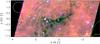 |
Fig. 3 Integrated intensity contours in 13CO 1–0 (green) and in [C i]
|
4. Interpretation
A full analysis of all the spatial and velocity structure visible in Fig. 1 goes beyond the scope of this paper. We provide only a first analysis, restricted to the 34 km s-1 component associated with the IRDC and start with some morphological considerations.
Ormel et al. (2005) identified three submm cores in the IRDC as possible sites of early massive star formation. They are located at offset positions of 1.26′, –0.05′ (P1), 0.80′, –0.18′ (P2), and 0.05′, –0.13′ (EP) marked by asterisks in Fig. 3 (see also Van der Wiel & Shipman 2008). These cores basically line-up along the horizontal filament in Fig. 3 and are also traced by the 13CO emission. Van der Wiel & Shipman (2008) identified 24 μm point sources in all three submm cores (P1 containing two sources), but also an additional strong 24 μm source at 1.35′, − 1.21′ (their S2, visible as blue point source in Fig. 3), south of P1, a position where no submm core was seen. This southern part of the cloud, traced by the IR extinction and the 13CO emission, is visible in the 850 μm continuum, but shows no pronounced condensations. The point sources in the western cores (P2 and EP) have not been detected in the IRAC bands while the point sources in the eastern core (P1) and the southern part show a significant flux even at 3.6 μm with the southern source also matching a 2MASS point source. This indicates that the latter are either in a more evolved state or at a somewhat lower column density relative to the observer.
Comparing this complementary information with the [C i] emission shows that [C i] neither traces the column density of the cloud nor is concentrated at the surfaces of the cloud, but that it is peaked at the sites of intense NIR radiation. If we assume that the large-scale structure of the IRDC, in particular the surface to volume ratio, is similar in all parts of the cloud, the internal, more evolved radiation sources remain as the main cause for the enhancement of atomic carbon. The very deeply embedded sources present in the western cores do not contribute to a local enhancement of atomic carbon, but as soon as the sources become visible in the NIR, they change the C i abundance. Nevertheless, we have to emphasise that we observe relatively small changes of less than a factor two in the [C i] intensity. The global C i distribution is still dominated by the overall structure of the IRDC reflecting the external illumination.
We can use the available complementary information on the structure of the IRDC and on the
physics of PDRs to get a rough estimate for the temperature of the cloud. In spite of some
differences, all PDR models predict that the bulk of atomic carbon is found at temperatures
between about 10 K and 25 K for sources with low or intermediate radiation fields (Le Bourlot 1993; Röllig
et al. 2007)1. Using these values we can
deduce the C i column density from a single line applying an LTE analysis. The LTE
emissivity of the [C i] transition varies between
3.7 × 10⁻¹⁷ and 7.6 × 10⁻¹⁷ K km s-1 cm2 for
temperatures between 10 and 25 K (6.2 × 10⁻¹⁷ K km s-1 cm2
at 15 K) and the critical density is about 103 cm-3. To minimise the
relative error of the column density due to the temperature uncertainty we use the geometric
mean of the two extremes, i.e. 5.3 × 10⁻¹⁷ K km s-1 cm2,
and obtain a column density estimate that should be accurate within a factor 1.4.
Table 1 summarises the results for four sets of effective beam temperatures, measured at the locations of the western core (EP), the eastern core (P1), the position of the southern 24 μm source (S2), and the map average. The observed range of [C i] brightness temperatures is reflected by atomic carbon column densities of 3 − 9 × 1016 cm-2. The corresponding beam-integrated optical depths are at most 0.25, so that we can neglect self-absorption effects.
Parameters derived at four example positions in the cloud.
Using a similar approach for the 13CO column densities is somewhat less accurate because the molecule exists over a much larger temperature range. Here, we can rely on the modelling of the G48.65–0.29 IRDC by Ormel et al. (2005). They found that only a very small part of the submm cores is heated to temperatures above 20 K while the majority of the gas is subject to temperatures between 10 and 15 K, i.e. in a range at the lower end of the typical temperatures of atomic carbon. This is somewhat counter-intuitive, as one would usually expect 13CO deeper in the cloud than atomic carbon at locations better shielded from the UV radiation and consequently also significantly colder. However, higher densities in the inner cloud also provide a more efficient gas-grain interaction that can heat the gas again, even allowing for non-monotonous temperature distributions. The LTE emissivity of the 13CO 1–0 transition is 7.4 × 10⁻¹⁶ K km s-1 cm2 at 20 K and 1.0 × 10⁻¹⁵ K km s-1 cm2 at 10 K (8.7 × 10⁻¹⁵ K km s-1 cm2 at 15 K), the critical density is well below 103 cm-3. Using again a mean conversion factor, i.e. 8.6 × 10⁻¹⁶ K km s-1 cm2 should be accurate within 20%. Assuming a 12CO/13CO abundance ratio of 65 (Langer & Penzias 1990), we can translate this into CO column densities and C i/CO abundance ratios. Applying the standard CO/H2 abundance ratio of 8 × 10⁻⁵ from Blake et al. (1987) gives also a rough estimate for the total column densities. They are consistent with the numbers obtained by Ormel et al. (2005) and Simon et al. (2006). All numbers are summarised in Table 1.
We find C i/CO abundance ratios between 0.07 and 0.13. The C i/CO abundance ratio previously measured in star-forming regions covers the range between about 0.03 and 32 (Mookerjea et al. 2006; Little et al. 1994; Sun et al. 2008). The values found for G48.65–0.29 are found at the lower end of this range and this is consistent with the picture of atomic carbon being produced by star-formation processes in which more quiescent clouds, without internal UV fields, show lower C i/CO ratios than more evolved, active star-forming sites.
The LTE analysis applied above ignores, however, the possible spatial separation of the regions dominating the [C i] and the 13CO 1–0 emission. A physically self-consistent model of the cloud can be obtained using the known density structure of the submm cores obtained by Ormel et al. (2005). The roughly spherical core structure is well approximated by the KOSMA-τ PDR model (Röllig et al. 2006). This model simulates a spherical cloud with a radial density profile given by a r-1.5 decay covering a factor five in radii around a core with constant density. Assuming external illumination by an isotropic UV radiation field and cosmic rays, the model computes the stationary chemical and temperature structure by solving the coupled detailed balance of heating, line and continuum cooling and the chemical network using the UMIST data base of reaction rates (Woodall et al. 2007) expanded by separate entries for the 13C chemistry (see Röllig et al. 2007, for details). The model configuration provides a good match to the quiescent cores in the IRDC and may reflect the situation for most of the material in the IRDC. Here, atomic carbon is produced in a layer at the surface of the dense material and in the more extended diffuse material. In the inner core the material is predominantly molecular.
This approach is, however, not appropriate for the cores with internal radiation sources,
P1 and S2, where we expect some additional atomic carbon production in the centres.
Consequently, the KOSMA-τ PDR model should be able to reproduce the
[C i]  CO 1–0 intensity ratio of about 0.3 found at
the extinction peak and in the cloud average, but will only provide a lower limit to the
[C i]/13CO ratio for the two warm cores. When comparing the line
ratios at the different positions (see Table 1), we
find that the internal radiation from P1 produces only a slight enhancement of the atomic
carbon abundance over the value produced by the external UV illumination while for the
southern source internal and external illumination provide similar contributions.
CO 1–0 intensity ratio of about 0.3 found at
the extinction peak and in the cloud average, but will only provide a lower limit to the
[C i]/13CO ratio for the two warm cores. When comparing the line
ratios at the different positions (see Table 1), we
find that the internal radiation from P1 produces only a slight enhancement of the atomic
carbon abundance over the value produced by the external UV illumination while for the
southern source internal and external illumination provide similar contributions.
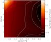 |
Fig. 4 [C i] |
Figure 4 shows the predicted intensity ratios as a function of cloud surface density and radiation field provided by the PDR extraction tool3 for the known core mass of about 100 M⊙ and solar metallicity4. White contours indicate the area of ratios matching the observed range. The ratio of about 0.3, i.e. lg{∫T([C i] )dv/∫T(13CO)dv} ≈ − 0.5, observed within most of the cloud and marked by the central white contour is only observed at high densities. For radiation fields in the order of the standard interstellar radiation field χ0 (Draine & Bertoldi 1996), a model with a clump surface density of about 3 × 104 cm-3 reproduces the observed ratio. The model predicts average temperatures of atomic carbon and 13CO of 12 K and 9 K, respectively, consistent with the estimates used above for the LTE analysis, but somewhat at the low edge as the model does not contain internal UV radiation sources.
When comparing the model with the results from the fit of the dust continuum and HCO+ emission by Ormel et al. (2005), we find a major discrepancy in the gas density. Ormel et al. (2005) derived surface densities of only about 103 cm-3. When taking internal clumpiness of the cores into account, local densities grow by a factor ten (core P1) or five (P2 and EP), but are still significantly lower than the model density fitting the [C i]/13CO ratio. For the lower densities, the KOSMA-τ model always predicts significantly higher line ratios. Models that assume a further break-up of the cores into smaller clumps have a higher surface to volume ratio, thus predicting even higher [C i]/13CO ratios. Lower ratios could be achieved for radiation fields significantly below the standard field χ0 but that would be hard to explain. Excitation from W51 can be excluded due to the large relative distance (Reid 1993) so that we expect fields in the order of χ0. A match could also be achieved when assuming unrealistically high metallicities Z > 3. With realistic parameters and the known masses and densities, the model predicts ratios above 0.5, only observed at the peaks with internal radiation sources where the model is expected to underestimate the ratio by neglecting this contribution. Invoking other model geometries than spherical clumps can only worsen the situation as they will always increase the surface to volume ratio of the cloud. Fractionation effects will hardly resolve the discrepancy as the KOSMA-τ PDR model includes the full 13C chemistry. But we have to admit that reaction rates for isotope-selective reactions are quite uncertain at low temperatures (see Röllig et al., in preparation). Thus, there is a clear contradiction between the measured [C i]/13CO line ratios and the model predicting higher values.
The same contradiction was noticed by Bensch et al. (2003) for the MCLD 123.5+24.9 translucent cloud. They suggested a pre-shielding by dust in a thin ionised gas as a possible solution. Time-dependent chemistry has been shown to tend towards the opposite direction, increasing the C i abundance (Störzer et al. 1997; Oka et al. 2004), but a fully time-dependent model, including turbulent mixing, still awaits development.
5. Conclusions
Our observations of [C i] in an IRDC showed an overall very good correlation
between atomic carbon and molecular gas, seen in 13CO 1–0, both in the spatial
and the velocity structure. This is naturally explained by a fractal cloud structure
illuminated by the external Galactic UV field (Ossenkopf
et al. 2007). The quantitative [C i]
 CO 1–0 ratios, however, cannot be explained
by available steady-state models. A spherical PDR clump model predicts higher line ratios
than observed. In a fractal structure with more internal surfaces, this ratio should even
grow further. More sophisticated models are needed. Future observations of the emission of
atomic oxygen at 4.7 THz may help to resolve the puzzle as [O i] is another,
independent tracer of illuminated, dense cloud surfaces.
CO 1–0 ratios, however, cannot be explained
by available steady-state models. A spherical PDR clump model predicts higher line ratios
than observed. In a fractal structure with more internal surfaces, this ratio should even
grow further. More sophisticated models are needed. Future observations of the emission of
atomic oxygen at 4.7 THz may help to resolve the puzzle as [O i] is another,
independent tracer of illuminated, dense cloud surfaces.
With the significant enhancement of the [C i] intensity observed towards the southern source, visible in the Spitzer IRAC bands, we can provide a first distinction between the roles of inner and outer PDRs if we assume that the outer structure is similar in all parts of the IRDC. A fraction of the [C i] emission comparable to that from the outer cloud surfaces, exposed to the interstellar radiation field, can be attributed to the internal radiation source. This means that any young stellar object that has created a sufficient cavity in the parental cloud, turning visible in the NIR, produces a considerable fraction of the total [C i] emission. For most of the star-forming regions observed so far in [C i], the emission will thus stem from inner surfaces.
Some uncertainties exist with respect to the temperature of the hottest few percent of atomic carbon, in particular in regions with high radiation fields. There, large differences exist between different PDR model predictions and this is also the range where the steady-state assumption used by most models is least justified. A parameter scan using the KOSMA-τ PDR model showed that higher average temperatures of atomic carbon can occur for n/M × χ ≳ 106 cm-3/M⊙χ0, i.e. for small dense clumps in a radiation field exceeding the average interstellar radiation field χ0. The known properties of the IRDC cores are sufficiently far apart from that boundary so that the uncertainties do not affect our estimate.
Lower values have been reported only towards the DR15 Hii region by Oka et al. (2001).
The web tool provides integrated line intensities in terms of photon energies, i.e. units of erg s-1 cm-2 sr-1. For intensity units of K km s-1, the conversion factor of 2kν3/c3 = 1.025 × 10⁻¹⁵(ν/GHz)3 has to be applied. This gives a conversion factor for the ∫T([Ci])dv/∫T(13CO)dv intensity ratio of 0.0112.
Acknowledgments
We thank two anonymous referees for many helpful comments. This work has been supported by the Deutsche Forschungsgemeinschaft through grant 494B. It has made use of NASA’s Astrophysics Data System Abstract Service.
References
- Bensch, F., Leuenhagen, U., Stutzki, J., & Schieder, R. 2003, ApJ, 591, 1013 [Google Scholar]
- Blake, G. A., Sutton, E. C., Masson, C. R., & Phillips, T. G. 1987, ApJ, 315, 621 [NASA ADS] [CrossRef] [Google Scholar]
- Draine, B. T., & Bertoldi, F. 1996, ApJ, 468, 269 [NASA ADS] [CrossRef] [EDP Sciences] [Google Scholar]
- Egan, M. P., Shipman, R. F., Price, S. D., et al. 1998, ApJ, 494, L199 [NASA ADS] [CrossRef] [Google Scholar]
- Falgarone, E., Hily-Blant, P., & Levrier F. 2004, ApSS, 292, 89 [Google Scholar]
- Graf, U. U., Heyminck, S., Michael, E. A., et al. 2003, SPIE, 4855, 32 [Google Scholar]
- Jackson, J. M., Rathborne, J. M., Shah, R. Y., et al. 2006, ApJS, 163, 145 [NASA ADS] [CrossRef] [Google Scholar]
- Kramer, C., Jakob, H., Mookerjea, B., et al. 2004, A&A, 424, 887 [NASA ADS] [CrossRef] [EDP Sciences] [Google Scholar]
- Ladd, E. F., & Covey, K. R. 2000, ApJ, 536, 380 [NASA ADS] [CrossRef] [Google Scholar]
- Langer, W. D., & Penzias, A. A. 1990, ApJ, 357, 477 [NASA ADS] [CrossRef] [Google Scholar]
- Le Bourlot, J., Pineau Des Forets, G., Roueff, E., & Flower, D. R. 1993, A&A, 267, 233 [NASA ADS] [Google Scholar]
- Little, L. T., Gibb, A. G., Heaton, B. D., Ellison, B. N., & Claude S. M. X. 1994, MNRAS, 271, 649 [NASA ADS] [CrossRef] [Google Scholar]
- Mookerjea, B., Kramer, C., Röllig, M., & Masur, M. 2006, A&A, 456, 235 [NASA ADS] [CrossRef] [EDP Sciences] [Google Scholar]
- Oka, T., Yamamoto, S., Iwata, M., et al. 2001, ApJ, 558, 176 [NASA ADS] [CrossRef] [Google Scholar]
- Oka, T., Iwata, M., Maezawa, H., et al. 2004, ApJ, 602, 803 [NASA ADS] [CrossRef] [Google Scholar]
- Ormel, C. W., Shipman, R. F., Ossenkopf, V., & Helmich, F. P. 2005, A&A, 439, 613 [NASA ADS] [CrossRef] [EDP Sciences] [Google Scholar]
- Ossenkopf, V., Röllig, M., Cubick, M., & Stutzki, J. 2007, in Molecules in Space and Laboratory, ed. J. L. Lemaire, & F. Combes (S. Diana publ.), 95 [Google Scholar]
- Pérault, M., Omont, A., & Simon, G. 1996, A&A, 315, L165 [NASA ADS] [Google Scholar]
- Pineda, J. L., & Bensch, F. 2007, A&A, 470, 615 [NASA ADS] [CrossRef] [EDP Sciences] [Google Scholar]
- Plume, R., Bensch, F., Howe, J. E., et al. 2000, ApJ, 539, L133 [NASA ADS] [CrossRef] [Google Scholar]
- Rathborne, J. M., Jackson, J. M., & Simon R. 2006, ApJ, 641, 389 [NASA ADS] [CrossRef] [Google Scholar]
- Rathborne, J. M., & Simon R., Jackson, J. M. 2007, ApJ, 662, 1082 [NASA ADS] [CrossRef] [Google Scholar]
- Reid, M. J. 1993, ARA&A, 31, 345 [NASA ADS] [CrossRef] [Google Scholar]
- Röllig, M., Ossenkopf, V., Jeyakumar, S., Stutzki, J., & Sternberg, A. 2006, A&A, 451, 917 [NASA ADS] [CrossRef] [EDP Sciences] [Google Scholar]
- Röllig, M., Abel, N. P., Bell, T., et al. 2007, A&A, 467, 187 [NASA ADS] [CrossRef] [EDP Sciences] [Google Scholar]
- Shipman, R. F., Frieswijk, W., & Helmich, F. P. 2003, in Galactic Star Formation Across the Stellar Mass Spectrum, ed. J. M. de Buizer, & N. S. van der Bliek, 252 [Google Scholar]
- Simon, R., Rathborne, J. M., Shah, R. Y., Jackson, J. M., & Chambers, E. T. 2006, ApJ, 653, 1325 [NASA ADS] [CrossRef] [Google Scholar]
- Störzer, H., Stutzki, J., & Sternberg, A. 1996, A&A, 323, L13 [Google Scholar]
- Sun, K., Ossenkopf, V., Mookerjea, B., et al. 2008, A&A, 489, 207 [NASA ADS] [CrossRef] [EDP Sciences] [Google Scholar]
- van der Wiel, M. H. D., & Shipman, R. F. 2008, A&A, 490, 655 [NASA ADS] [CrossRef] [EDP Sciences] [Google Scholar]
- Winnewisser, G., Bester, M., & Ewald, R. 1986, A&A, 167, 207 [NASA ADS] [Google Scholar]
- Woodall, J., Agúndez, M., Markwick-Kemper, A. J., & Millar, T. J. 2007, A&A, 466, 1197 [NASA ADS] [CrossRef] [EDP Sciences] [Google Scholar]
Appendix A: Effects of extended emission
Both 13CO and [C i] are known to show very extended emission so that it needs to be investigated to which degree the measured intensity at each point may be affected by this emission. Two effects have to be considered: self-chopping and intensity pick-up by the extended error beam. Taken the similarity of the emission of 13CO and [C i] we can estimate these effects from the larger 13CO 1–0 FCRAO map showing also the environment of the IRDC. It is displayed in Fig. A.1 using the same integration range as in Fig. 3.
The [C i] observations were taken in double beam-switch mode using a fixed chop throw of 6′ in azimuthal direction. The sky rotation relative to the azimuthal direction then leads to variable OFF positions depending on date and time of the observation. In Fig. A.1 we have indicated the area of OFF maps covered in the course of the observation runs. We see that the centre of the map is never affected by self-chopping effects, but that the north-west corner and the east edge of the map could be affected by self chopping. As we have not detected any significant [C i] emission at these points, this might only mean that [C i] is slightly more extended than shown in Fig. 3.
We have to admit, however, that the spectra show some self-chopping effects at frequencies out of the considered velocity interval. This can be seen as negative features around 44 km s-1 in some spectra in the south-west part of the map and around 55 km s-1 in the south of the map. These contributions stem from gas components south-east of the IRDC. As all these features only show up outside of the velocity integration interval assigned to the IRDC, self chopping effects can be neglected for the integrated [C i] intensities.
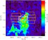 |
Fig. A.1 Map of the large-scale emission as measured by the 13CO 1–0 line. The map covered by [C i] observations is shown as gray rectangle in the centre, the brown rectangles around that map indicate the locations of the OFF maps taken in the double beam-switch scheme at the different times and dates of the observations. The circle indicates the size of the KOSMA error beam at the [C i] frequency. The FCRAO error beam at the 13CO 1–0 frequency is smaller by a factor three and is not shown here. |
The extended emission will also lead to additional intensity pick-up in the error beams of the telescopes. The error beam of the KOSMA telescope, produced by a slight misalignment of the individual panels has a size of about 330′′ (Kramer et al. 2004). Comparing the moon efficiency of 80% to the main beam efficiency of 62% provides a maximum error beam efficiency of 18%. We have estimated the error beam pickup by convolving the FCRAO map with a 330′′ Gaussian, weighted by the error beam efficiency, and comparing it to the map values weighted by the main beam efficiency. We find that at the emission peaks, the error beam contribution falls between 8 and 12%, over most of the map it amounts to about 15% but it reaches a value of 30% at the south-west corner of the map. Consequently, the true [C i] emission might be somewhat less extended in the south-west direction than shown in Fig. 3. Due to the error-beam pickup we overestimate the local emission when dividing the measured intensity by the main-beam efficiency only. Using an effective beam efficiency of 69% instead of 62% gives a correction for this effect that should be accurate to about 10% over most of the observed map.
The error beam of the FCRAO telescope at the 13CO 1–0 frequency has a width of about 100′′. The main beam efficiency is about 48% and the measured moon efficiency 72% (Ladd & Covey 2000). Repeating the deconvolution exercise for this smaller error beam gives a relatively constant ratio of about 0.45 for most of the map which is only slightly smaller than the ratio between error beam and main beam efficiency. Consequently, we will use a value of 70%, only slightly below the moon efficiency as the effective beam efficiency to calibrate the 13CO.
This approach may slightly underestimate the intensity as the moon efficiency is only an upper limit for the sum of main-beam and error-beam efficiency and some small components at the scale of a few arcminutes might contribute, but the residual error from this contribution will certainly fall below 10%.
All Tables
All Figures
|
Fig. 1 Line profiles measured on 13CO 1–0 (black, BU-FCRAO Galactic Ring Survey)
and in [C i] |
| In the text | |
|
Fig. 2 Scatter plot of the measured 13CO and [C i] intensities for different channels and points across the cloud. The red line indicates a [C i]/13CO intensity ratio of 1/3. |
| In the text | |
|
Fig. 3 Integrated intensity contours in 13CO 1–0 (green) and in [C i]
|
| In the text | |
|
Fig. 4 [C i] |
| In the text | |
|
Fig. A.1 Map of the large-scale emission as measured by the 13CO 1–0 line. The map covered by [C i] observations is shown as gray rectangle in the centre, the brown rectangles around that map indicate the locations of the OFF maps taken in the double beam-switch scheme at the different times and dates of the observations. The circle indicates the size of the KOSMA error beam at the [C i] frequency. The FCRAO error beam at the 13CO 1–0 frequency is smaller by a factor three and is not shown here. |
| In the text | |
Current usage metrics show cumulative count of Article Views (full-text article views including HTML views, PDF and ePub downloads, according to the available data) and Abstracts Views on Vision4Press platform.
Data correspond to usage on the plateform after 2015. The current usage metrics is available 48-96 hours after online publication and is updated daily on week days.
Initial download of the metrics may take a while.