| Issue |
A&A
Volume 524, December 2010
|
|
|---|---|---|
| Article Number | A56 | |
| Number of page(s) | 17 | |
| Section | Extragalactic astronomy | |
| DOI | https://doi.org/10.1051/0004-6361/201015338 | |
| Published online | 23 November 2010 | |
NGC 6240: merger-induced star formation and gas dynamics⋆
1
Max Planck Institut für extraterrestrische Physik,
Postfach 1312,
85741
Garching,
Germany
e-mail: This email address is being protected from spambots. You need JavaScript enabled to view it.
2
Universitätssternwarte, Scheinerstrasse 1, 81679
München,
Germany
3
Center for Adaptive Optics, University of California,
Santa Cruz,
CA
95064,
USA
4
Leiden Observatory, Leiden University,
PO Box 9513,
2300 RA
Leiden, The
Netherlands
Received: 5 July 2010
Accepted: 26 August 2010
Abstract
We present spatially resolved integral field spectroscopic K-band data at a resolution of 0.13″ (60 pc) and interferometric CO(2–1) line observations of the prototypical merging system NGC 6240. Despite the clear rotational signature, the stellar kinematics in the two nuclei are dominated by dispersion. We use Jeans modelling to derive the masses and the mass-to-light ratios of the nuclei. Combining the luminosities with the spatially resolved Brγ equivalent width shows that only 1/3 of the K-band continuum from the nuclei is associated with the most recent star forming episode; and that less than 30% of the system’s bolometric luminosity and only 9% of its stellar mass is due to this starburst. The star formation properties, calculated from typical merger star formation histories, demonstrate the impact of different assumptions about the star formation history. The properties of the nuclei, and the existence of a prominent old stellar population, indicate that the nuclei are remnants of the progenitor galaxies’ bulges.
Key words: galaxies: active / galaxies: individual: NGC 6240 / galaxies: interactions / galaxies: evolution / galaxies: star formation / galaxies: starburst
Based on observations at the European Southern Observatory VLT (079.B-0576).
© ESO, 2010
1. Introduction
Major mergers are key drivers of galaxy evolution. Profoundly transformational events, they substantially affect virtually all properties of a galaxy. Mergers between disc galaxies are believed to be responsible for triggering galaxy-wide starbursts (Toomre & Toomre 1972; Mihos & Hernquist 1996; Genzel et al. 1998a,b; Veilleux et al. 2002; Springel et al. 2005; Hopkins et al. 2006), quasar activity (Sanders et al. 1988a,b; Sanders & Mirabel 1996; Veilleux et al. 2002; Jogee 2004; Springel et al. 2005; Dasyra et al. 2006b; Hopkins et al. 2006, 2008), and the creation of elliptical galaxies (Toomre & Toomre 1972; Toomre 1977; Kormendy & Sanders 1992; Mihos & Hernquist 1996; Genzel et al. 2001; Dasyra et al. 2006a,b).
Star formation activity in merging gas-rich galaxies peaks between first peripassage and final coalescence (Sanders & Mirabel 1996; Mihos & Hernquist 1996; Veilleux et al. 2002; Springel et al. 2005). Due to absorption and re-emission by dust, almost all of this energy is emitted at infrared wavelengths, giving rise to extremely high infrared luminosities. Objects with LIR = 1011−11.9 L⊙ are called luminous infrared galaxies (LIRGs), those with LIR ≥ 1012 L⊙ ultraluminous infrared galaxies (ULIRGs). The local LIRG population consists of both (typically early-stage) mergers and non-interacting galaxies (Sanders 1992; Alonso-Herrero et al. 2006), whereas local ULIRGs are almost always interacting galaxies beyond first encounter (Sanders et al. 1988a; Sanders & Mirabel 1996; Veilleux et al. 2002; Jogee 2004). Local ULIRGs are predominantly powered by the starburst, except for the most luminous objects (Genzel et al. 1998b).
Despite their recognised importance, we still lack a good understanding of merger processes. This is due both to the complexity and the shortlived nature of these events. A rare opportunity to study the transient phase between first encounter and final coalescence of two merging gas-rich spirals is afforded by NGC 6240, at a distance of 97 Mpc. With LIR ~ 1011.8 L⊙ (Sanders & Mirabel 1996), it falls just short of being formally classified as a ULIRG. HST images show a large-scale morphology dominated by tidal arms characteristic for mergers past first peripassage (Gerssen et al. 2004). It is therefore more characteristic of the ULIRG class, to which it is commonly assigned; and our analysis shows its luminosity is likely to exceed the ULIRG threshold in the next 100–300 Myr. Two distinct nuclei, with a projected separation of ~1.5″ or 700 pc, are seen at infrared, optical, and radio wavelengths (Tecza et al. 2000; Max et al. 2005, 2007; Gerssen et al. 2004; Beswick et al. 2001). Each nucleus is host to an AGN, detected in hard X-rays (Komossa et al. 2003) and at 5 GHz (Gallimore & Beswick 2004). However, Lutz et al. (2003) and Armus et al. (2006) estimate that the AGN contribute less than half, and perhaps only 25%, of the luminosity. Tacconi et al. (1999) find the cold gas, as traced by CO(2–1) emission, to be concentrated between the two nuclei. The 1-0 S(1) H2 line emission is one of the most powerful found in any galaxy to date (Joseph et al. 1984), probably excited in shocks (van der Werf et al. 1993; Sugai et al. 1997; Tecza et al. 2000; Lutz et al. 2003). The stellar kinematics (Tecza et al. 2000) display rotation centred on each of the two nuclei, and extraordinarily large stellar velocity dispersions (~350 km s-1) between them. Tecza et al. (2000) find evidence for a recent starburst in the central kpc (the region encompassing the two nuclei), and Pollack et al. (2007) resolve a few dozen clusters in the nuclear region that are also consistent with a recent starburst.
In this paper we build on the qualitative picture put forward by Tecza et al. (2000) that NGC 6240 is a merger already past its first close encounter, where the luminosity arises from a very recent burst of star formation, and therefore in which the mass must be due to an older stellar population. We use new adaptive optics integral field K-band spectra, interferometric mm CO(2–1) data, and merger star formation histories from numerical simulations, to perform a quantitative analysis of the mass, luminosity, age, and origin of the young and old stellar populations.
We first introduce the observations and data reduction processes for the data sets used in our analyses (Sect. 2). We briefly look at the molecular gas (Sect. 3), and then focus on a detailed analysis of the stellar dynamics (Sects. 4–7), before discussing the merger geometry and stage, and the curious CO(2–1) morphology (Sect. 8). Bringing together these results, we then investigate the scale of the starburst (Sect. 9) and nature and origin of the nuclei (Sect. 10). We summarise our results in Sect. 11.
2. Observations and data processing
2.1. SINFONI data
2.1.1. Observations and reduction
Observations of NGC 6240 were performed on the night of 20 Aug 2007 at the Very Large Telescope (VLT) with SINFONI. SINFONI is a near-infrared integral field spectrometer (Eisenhauer et al. 2003) which includes a curvature-based adaptive optics system (Bonnet et al. 2004). For these observations the wavefront reference was provided by the Laser Guide Star Facility (Bonacini Calia et al. 2006; Rabien et al. 2004). We used the R = 13.7 mag star 40″ off-axis from NGC 6240 to correct for tip-tilt motions. The instrument was rotated by 70° east of north in order to acquire this star. In order to cover both nuclei of NGC 6240 simultaneously, the 0.05″ × 0.10″ pixel scale was chosen, giving a 3.2″ × 3.2″ field of view. This pixel scale and the K-band grating provide a resolution of 6.6 × 10⁻⁴ μm, equivalent to R ~ 3300 or 90 km s-1FWHM at 2.18 μm.
The data set comprised 12 object frames interleaved with 4 sky frames. Each exposure was 300 s, yielding a total on-source integration time of 60 min. Data were reduced using the dedicated SPRED software package (Abuter et al. 2006), which provides similar processing to that for long-slit data but with the added ability to reconstruct the data cube by stacking the individual slitlets. In order to optimise the sky subtraction, we made use of the algorithm described in Davies (2007). The image was rotated to restore the standard orientation, with north along the Y-axis, and east along the X-axis. The pixel scale of the final reduced cube was 0.05″ × 0.05″.
Standard star frames were similarly reconstructed into cubes. Telluric correction and flux calibration were performed using HD 147550, a B9 V star with K = 5.96 mag. Velocity Standards were also observed with the same spatial and spectral settings, in order to enable recovery of the kinematics. The 3 stars observed, and added to our library of similar stars, were HD 176617 (M3 III), HD 185318 (K5 III), and HD 168815 (K5 II). These stars were chosen because of their deep CO absorption longward of 2.3 μm which provides a good match to that of NGC 6240.
2.1.2. PSF estimation
We estimate the PSF by comparing the SINFONI data to higher resolution K-band Keck AO imaging data (Pollack et al. 2007), which are both shown in Fig. 1. Although the spatial resolution of our integral field observations is not as good as that achieved by these Keck imaging data, we note that the two bright spots in the northern nucleus are clearly separated in our data, indicating that our resolution is better than the 0.2″ achieved by HST/NICMOS (Fig. 3c in Gerssen et al. 2004).
As outlined by Davies (2008) and employed by Mueller Sánchez et al. (2006), since an observed image is the convolution of an intrinsic image with a PSF, Iobs = Iintr ⊗ PSF, we can use a higher resolution image with a known PSF to obtain a good estimate of the PSF in a lower resolution image in two steps. Having resampled the data to the same pixel scale, we first find the broadening function B whose convolution with the high resolution image yields the best match to the low resolution image, Ilow = Ihigh ⊗ B. Since the underlying intrinsic image is the same for both Ilow and Ihigh, we can then estimate the PSF of the low resolution image by convolving the broadening function B with the PSF of the high resolution image, PSFlow = PSFhigh ⊗ B. Since in this case B dominates the size and shape of our PSF, uncertainties in PSFhigh have little impact on PSFlow. For the analyses carried out here, this procedure gives a sufficiently accurate definition for the PSF. We find the PSF to be well matched by an asymmetric Gaussian with major axis oriented −20° east of north. The resolution is 0.097″ × 0.162″ FWHM, corresponding to 50 × 80 pc at the distance of NGC 6240. The asymmetry is to be expected since the resolution of the original data is pixel limited, being sampled at 0.05″ × 0.10″. The reason we are able to do better than the formal Nyquist limit is because the SINFONI data are resampled to 0.05″ × 0.05″ and many dithered exposures are combined using sub-pixel shifts to align them.
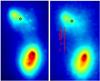 |
Fig. 1 K-band adaptive optics images of NGC 6240 in square-root colour scale. Left: K-band flux density from NIRC2 on Keck II (pixel scale 0.01″, Pollack et al. 2007; Max et al. 2007). Right: 2.2 μm continuum from SINFONI on the VLT (pixel scale 0.05″), covering approximately the same field as left. In both panels, circles indicate AGN positions (see Sect. 5), north is up and east is left, and the red bar indicates 1″ (500 pc). |
2.1.3. Spatial binning
Because of the limited signal-to-noise in our data, we have binned them spatially using an optimal Voronoi tessellation (Cappellari et al. 2003). This algorithm bins pixels together into groups by accreting new pixels to each group according to how close they are to the centroid of the current group. The resulting groups then provide a set of positions (centroids) and mean fluxes which are used as the initial “generators”. A further algorithm optimises the generator configuration based on a centroidal Voronoi tessellation. The final set of generators are the positions of the flux-weighted centroids of each binned group, and have the property that each pixel in the original image is assigned to the group corresponding to the nearest generator. This procedure only affects spaxels below a specified signal-to-noise threshold, and hence does not impact the spatial resolution of high signal-to-noise regions. The signal-to-noise cutoff was 20, chosen such that the regions with the highest signal-to-noise remained fully sampled, but lower signal-to-noise regions were binned. This avoided compromising the spatial resolution around the center of each nucleus, while enabling us to extend the region in which analyses can be performed. The effect of this can be seen in the resulting stellar kinematics maps, where the colours in the outer regions appear in blocks rather than individual pixels. The binning scheme that this routine provided was applied to each spectral plane in the cube, and the kinematics were extracted from each bin as described below.
2.1.4. Extracting stellar kinematics
The observed wavelength regime contains the stellar CO absorption bandheads longward of 2.29 μm, whose sharp blue edges are very sensitive to stellar motions. We utilise CO 2–0 and CO 3–1 to derive 2D maps of the stellar velocity and dispersion. The spectra were prepared by normalising them with respect to a linear fit to the line-free continuum. The continuum level was then set to zero by subtracting unity. A template spectrum, that of the M3 III star HD 176617, was prepared in the same way. Although both Sugai et al. (1997) and Tecza et al. (2000) used K Ib stars, they also both noted that M III stars provided almost equally good fits to the K-band features (see Fig. 5 in Tecza et al. 2000). We therefore do not expect template mismatch to be a problem but, as explained below, our method furthermore minimises the impact of any discrepancy. Silge & Gebhardt (2003) showed that the dispersion measured depends on the equivalent width of the template; this can be understood since the depth of the extinction feature relative to the continuum level (which may contain non-stellar emission) places a strong constraint on the fitting parameters. But it is the spectral width, not the equivalent width (i.e. depth), of the absorption feature that is important for deriving the dispersion.
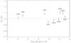 |
Fig. 2 The ratio between the measured dispersion σout and the input dispersion σin for a range of different stellar templates used to extract kinematics from a K 5Ib template. For each combination, a variety of dispersions in the range 150–300 km s-1 were used and noise was added to achieve a S/N ~ 35. Variations in measured stellar kinematics using templates with a large range of WCO and stellar types are around a few percent, showing that with our method a mismatched stellar template has little effect. |
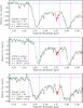 |
Fig. 3 Spectra (black lines) and template fits (green lines) to the CO 2–0 and CO 3–1 stellar absorption features. These are for individual bins in the southern nucleus (top), the northern nucleus (middle) and in the region of high dispersion between them (bottom). The blue line indicates the continuum (i.e. zero) level; red asterisks denote pixels rejected during the fit; the pairs of magenta lines enclose regions around the bandheads for which the weighting is enhanced during the fit. These plots demonstrate the quality of the fit using our single M3 III template. |
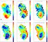 |
Fig. 4 Stellar velocity and corresponding noise map (top and bottom left, both in km s-1 with respect to systemic), dispersion and corresponding noise map (middle, both in km s-1), and WCO2−−0 and its noise map (right, both in Å). Contours trace the continuum as in Fig. 1. Black/magenta circles mark the AGN positions (see Sect. 5). The bar indicates 1″ (images are 2.45″ × 3.95″), the PSF size is shown in the lower left corner of panel 1. North is up and east is to the left. |
In order to demonstrate this quantitatively, we have made use of the stellar template library of Winge et al. (2009). We created a large series of mock observations by broadening a K5 Ib template by various amounts in the range 150–300 km s-1, and adding noise. We then extracted the dispersion using various mis-matched stellar templates spanning a wide range of WCO (equivalent width of the CO absorption feature) and spectral type. As can be seen in Fig. 2, our method recovers the input dispersion with a typical error of only a few percent, regardless of the template’s spectral type. This shows that our method of extracting the stellar kinematics works reliably even if the template used is not a perfect fit. We emphasize that, in contrast to Sugai et al. (1997) and Tecza et al. (2000), we do not use the quality of the template fit to draw conclusions about the prevalent stellar population. This requires caution, and we discuss the pitfalls associated with doing so in Sect. 9. As such, because we use this star only for extracting kinematics, our choice of template can be fully justified by the good fits to the bandheads in the galaxy spectra in Fig. 3.
For the spectrum at each spatial pixel (“spaxel” hereafter) in the data cube, we convolve the template with a Gaussian, adjusting the properties of the Gaussian to minimise the difference between the convolution product and the galaxy spectrum. Deviant pixels are rejected from the fit. The spectral regions covering the steep edges of the bandhead at all expected stellar velocities are given five-fold weight (Fig. 3), in order to focus the fit on the kinematics rather than details in the spectrum. To ensure consistency in our analyses, the spectral ranges applied to compute WCO were taken from Förster Schreiber (2000), since these ranges are also used by the stellar synthesis code STARS which we use later. A high signal-to-noise (≳50, Cappellari et al. 2009) is required in order to measure deviations in the line of sight velocity distribution from a simple Gaussian. Without binning beyond a useful spatial resolution, the signal-to-noise in most of our spectra is not sufficient to include the Gauss-Hermite terms h3 and h4 in the fit. We therefore limited the kinematic extraction to V and σ. The noise in the kinematics was determined using Monte Carlo techniques: 100 realisations of the data were generated, a number that ensures a fractional uncertainty in the noise of less than 10%, by perturbing the flux at each pixel according to its RMS. These were fit using the same procedure as above. Although the RMS at each pixel can be derived when combining the data cubes, calculating the noise in bins is extremely difficult due to the correlations between neighbouring pixels. This is discussed in detail by Förster Schreiber et al. (2009). Instead, we have derived the noise as the RMS of the difference between a spectrum and the convolved template (excluding rejected pixels). This may slightly over-estimate the noise, but will then yield conservative error estimates on the kinematic parameters. The resulting final maps of stellar velocity, dispersion, and WCO2−0 are displayed in Fig. 4.
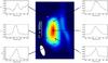 |
Fig. 5 Map of CO(2–1) flux with spectral line profiles shown for selected spaxels. Circles denote AGN positions, stars denote positions where spectra were extracted. The beam size is displayed in lower left. The bar denotes 1″, and north is up and east is to the left. |
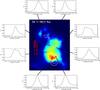 |
Fig. 6 Map of H2 1-0 S(1) emission, with line shapes at selected spaxels. Circles mark AGN positions, stars denote positions where spectra were extracted, white contours represent continuum emission. The bar denotes 1″, and north is up and east is to the left. |
2.2. Plateau de bure interferometer data
We have mapped the 12CO(J = 2–1) line in NGC 6240 with the IRAM millimetre interferometer, which is located at an altitude of 2550 m on the Plateau de Bure, France (Guilloteau et al. 1992). The data were obtained in May 2007. The array consisted of six 15 m antennae positioned in two configurations providing a large number of baselines ranging from 32 to 760 m. We observed NGC 6240 for 5 h in A configuration, which provides a nominal spatial resolution of 0.35″ at 230 GHz. However, the low (+2 deg) declination of NGC 6240 limited the resolution in an approximately north-south direction. A spectral resolution of 2.5 MHz, corresponding to 3.3 km s-1 for the CO(2–1) line, was provided by 8 correlator spectrometers covering the total receiver bandwidth of 1000 MHz (1300 km s-1). All the data were first calibrated using the IRAM CLIC software. We then made uniformly weighted channel maps for the CO(2–1) data. We CLEANed all the maps using software available as part of the GILDAS package. To increase the sensitivity, maps were made with a velocity resolution of 26.6 km s-1. The CLEANed maps were reconvolved with a 0.69″ × 0.26″ FWHM Gaussian beam. The rms noise after CLEANing is 1.4 mJy beam-1. Figure 5 shows the velocity-integrated CO(2–1) emission (black circles denoting approximate AGN locations), velocity moment map, and the dispersion (obtained from fitting Gaussians to the line shape). The AGN positions were estimated using the positions given by Gallimore & Beswick (2004); due to the astrometric uncertainties, these are only accurate to within 1–2 pixels (0.7–0.14″).
3. Molecular gas emission
3.1. H2 1-0S(1)
NGC 6240 has the strongest H2 line emission found in any galaxy to date (Joseph et al. 1984). Several authors (van der Werf et al. 1993; Sugai et al. 1997; Tecza et al. 2000) identify shocks as the excitation mechanism, and Ohyama et al. (2003) use the relative intensity of H2 and CO(2–1) emission to conjecture that the shocks occur due to a superwind outflowing from the southern nucleus colliding with the molecular gas concentration. Our new SINFONI data provide the most detailed spatial and spectral view currently available. As can be seen in Fig. 6, the line profiles are highly complex, with clear evidence of multiple components. This, and the dispersion map (Fig. 7), support the picture of highly disturbed, turbulent gas. The emission morphology is uncorrelated with the stellar emission distribution, but roughly consistent with the cold gas emission (as traced by the CO(2–1) emission, Sect. 3.2). The velocity moment map (Fig. 7) shows a global velocity gradient, again broadly consistent with what is seen in CO(2–1).
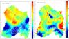 |
Fig. 7 Velocity moment (left) and dispersion (right) maps of H2. Magenta circles mark AGN positions, white contours represent H2 1-0 S(1) line emission. |
3.2. CO(2–1)
Figure 5 shows the velocity-integrated CO(2–1) emission, with line shapes at selected positions. With a factor of two improvement in resolution along the E-W direction, our data re-affirm the findings of Tacconi et al. (1999). However, our resolution in the crucial N-S direction is limited by the declination of the source. As a result we are not able to draw more detailed conclusions about the CO(2–1).
The CO emission is concentrated in between the two nuclei, and the CO(2–1) velocity map, red and blue wings, and P-V-diagram all display signs of a velocity gradient. This is consistent with the findings of Tacconi et al. (1999), who conclude that the molecular gas likely is concentrated in a self-gravitating rotationally supported, but highly turbulent disc in the internuclear region. However, such a central gas concentration is not expected from merger simulations, which generally predict the gas to remain largely bound to the progenitors until the nuclei coalesce. We discuss this issue further in Sect. 8.
The total flux is about 40% less than that measured by Tacconi et al. (1999), indicating that our smaller beam has resolved out some emission on intermediate to large scales. We have not made a correction for this, since we are interested primarily in the small scale emission of the nuclei themselves, where the effect is likely to be negligible. To estimate the gas mass associated with the nuclei, we have measured velocity-integrated line fluxes within the same radii as those used in our dynamical mass modelling (Sect. 7), which were chosen to cover the extent of observed stellar rotation in the nuclei. In the northern nucleus we find SCOΔV = 37 Jy km s-1 out to a radius of 250 pc; in the southern nucleus we find SCOΔV = 178 Jy km s-1 out to a radius of 320 pc.
We estimate the gas mass by converting to line luminosity  (with DL = 97 Mpc, z = 0.0243, νobs,CO2−1 = 225.1 GHz), and using the relations L(CO2−1)/L(CO1−0) = 0.8 (Casoli et al. 1992) and MH2/LCO1−0 ~ 1 M⊙/(K km s-1 pc2), as Downes & Solomon (1998) find for ULIRGs. This yields ~0.2 × 10⁹ M⊙ and ~1.1 × 10⁹ M⊙ for northern and southern nuclei, respectively. Similarly, for an aperture of 1″ diameter centred on the CO emission peak, we derive a gas mass of ~3.1 × 10⁹ M⊙. We caution that the nuclear masses are very uncertain and should be treated only as order-of-magnitude estimates. The reason is that a significant fraction of the gas within the apertures may not be physically co-located with the nuclei, which would imply the masses are upper limits. On the other hand, the CO abundance around the nuclei is very likely to have been significantly reduced by X-ray irradiation from the AGN (see Sect. 8). In this case, the masses would be underestimates.
4. Extinction and luminosity of nuclei
Like most ULIRGs, NGC 6240 contains significant amounts of dust (Tecza et al. 2000), and hence correcting any flux measurement for extinction is paramount to ensure accuracy in the analyses described below. It is valuable to consider the extinction derived from mid-infrared data to assess whether the near infrared might be affected by saturation. However, this appears to be uncertain – primarily because no Hii lines were detected either by ISO (Lutz et al. 2003) or Spitzer (Armus et al. 2006). Based on silicate absorption at 9.7 μm, Armus et al. (2006) find an extinction of AV ~ 95 mag to the coronal line region. The more moderate estimates presented by Lutz et al. (2003) are for a global extinction, and correspond to a dust screen AV ~ 15−20 mag. This estimate is comparable to derivations at radio (NH ~ (1.5−2) × 1022 cm-2, Beswick et al. 2001) and X-ray (NH ~ 1022 cm-2, Komossa et al. 2003) wavelengths. This is important, because it implies a modest typical K-band screen extinction of only AK ~ 1−2 mag. Thus our data should be sensitive to the majority of the emission. However, we note that the X-ray spectrum at energies above 10 keV indicates that at least one of the AGN themselves may be obscured by a column >1024 cm-2 (Vignati et al. 1999; Ikebe et al. 2000; Netzer et al. 2005). Differences between these various column density measurements are to be expected since they sample different spatial scales and sight lines; for example, the X-ray data specifically measure gas column density along the line of sight to the AGN rather than the extended cold dusty medium.
When correcting for the obscuring effect of dust, one needs to make assumptions about its location and distribution. The two most commonly used models assume either a uniform dust screen between the observer and the stars, leading to a reduction in observed flux according to Fobs/Fem = e−τ. Or the stars and dust are assumed to be spatially coincident and uniformly mixed (“mixed model”), in this case the observed flux decreases as Fobs/Fem = (1 − e−τ)/τ. Another alternative is the Calzetti et al. (2000) reddening law, derived empirically from observations of starburst galaxies. Its wavelength dependence reflects both the dust grain properties and the distribution of the dust with respect to the stars in these galaxies. The effect of this reddening law is remarkably similar to a combination of mixed and screen extinction, with – for the degree of extinction seen in NGC 6240 – the mixed component dominating in the infrared, and the screen component increasingly important at optical wavelengths. In order to investigate which extinction model best captures the characteristics of the dust distribution of NGC 6240, we obtained a number of archival HST imaging data, spanning wavelengths from 0.45 μm to 2.22 μm, and extracted photometric data points from a number of 0.2″ radius apertures across our field of view. And we calculated a synthetic stellar spectrum using the stellar synthesis code STARS (Sternberg 1998; Sternberg et al. 2003; Förster Schreiber et al. 2003; Davies et al. 2003, 2005, 2006, 2007), assuming a star formation rate typical for a merger (“Antennae”-simulation, Sect. 8). We then fitted this spectrum to the HST data points and our SINFONI K-band spectra, using the screen and mixed extinction models, and the Calzetti et al. (2000) reddening law. As can be seen in Fig. 8, the Calzetti et al. (2000) reddening law best reproduces the observations; the mixed model saturates at optical wavelengths and cannot redden the spectra sufficiently, and the screen model is reddening the spectra too much at shorter wavelengths. We also test whether our choice of star formation history has an influence on this result, by conducting the same test with synthesised spectra for a 20 Myr old instantaneous starburst and 1 Gyr of continuous star formation. Both also indicate the Calzetti et al. (2000) reddening law to be appropriate.
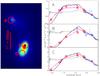 |
Fig. 8 Comparison of different extinction models: we measured HST photometric data points (red squares) in 0.2″ radius apertures; positions for the three examples shown here are indicated in the left panel. To these we fitted a synthetic STARS spectrum which was reddened using different reddening prescriptions: screen extinction (black), mixed extinction (grey), and the Calzetti et al. (2000) reddening law (magenta). We also overplot our SINFONI spectrum (blue), scaled to the HST 2.22 μm data point (absolute SINFONI flux at 2.2 μm shown as blue diamond). As can be seen, the Calzetti et al. (2000) reddening law provides the best fit to the data. |
We can then find Fobs/Fem for each spatial pixel by adjusting the reddening for a set of stellar template spectra according to Eq. (2) in Calzetti et al. (2000), until the best-fit of a linear combination of templates to the measured line-free continuum is achieved. Figure 9 shows the resulting map of AK. The choice of stellar templates does not affect the result, since the K-band samples the Rayleigh-Jeans tail of the blackbody curve and hence to a good approximation all stars, and late-type stars in particular, have the same spectral slope.
One might ask whether a component of non-stellar emission from hot dust might be present, in our field of view in general and close to the AGN in particular. This is an important question, since it would have an influence on the stellar masses and mass-to-light ratios we calculate later on. That the K-band continuum may even be dominated by hot dust has been proposed by Armus et al. (2006). However, this conclusion was based on a fit to the near-IR spectral energy distribution that was constrained primarily as the residual in the blue side of a much more dominant cooler component, and is therefore rather uncertain. Instead, the good match of reddened synthetic stellar spectra to the photometry (Fig. 8) indicates that non-stellar emission is unlikely to contribute significantly. More importantly, emission from hot dust would dilute the stellar CO absorption features. Since we measure WCO2−0 ~ 12−13 Å (Fig. 4), and the theoretically possible (achievable only through a 10 Myr old instantaneous starburst) maximum is ~18 Å, this puts a firm theoretical upper limit of < 30% on any non-stellar contribution, and realistically makes anything larger than a few percent unlikely. And since we do not see a localised dip in WCO2−0 around the AGN positions, we conclude that any hot dust emission associated with the AGN is completely obscured at near-IR wavelengths.
Table 1 lists the observed and dereddened luminosities measured within apertures of diameter 1″ centered on the northern and southern nuclei, from Tecza et al. (2000), this work, and from archival NICMOS data; and also those obtained by integrating the luminosity profiles out to 250 pc. We included the NICMOS data to obtain a third independent measurement, since our measurements of the observed luminosities and those of Tecza et al. (2000) differ by a factor of two. We find the NICMOS data agree with our measurements to within 10%. As can be seen, for Tecza et al. (2000), the dereddening only alters the measured luminosities by ~10%, whereas for us, the difference is circa a factor of two. This difference is most likely due to the fact that we applied a spatially dependent, rather than single-valued, correction.
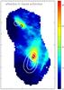 |
Fig. 9 Effective K-band extinction AK. As for Fig. 1, contours trace the continuum and black circles denote the AGN positions. Each 0.05″ pixel length corresponds to 25 pc at the distance of NGC 6240. |
Integrated luminosities of the nuclei
5. Kinematic centres and black hole locations
In this section, we attempt to confirm the hypothesis that the black hole locations do identify the centres of the progenitors, by independently determining the locations of the kinematic centres from the stellar velocity field. As we outline below, for a number of reasons locating the kinematic centres of the observed stellar rotation reliably and accurately is extremely difficult to do. Nevertheless, within the uncertainties, we find that the BH positions of Max et al. (2007) are consistent with the kinematic centres.
Max et al. (2007) determined the positions of the two AGN in NGC 6240 by combining images taken in the near-infrared, radio, and X-ray regimes. Postulating that the southern sub-peak of the northern nucleus as seen in the K-band (“N1” in the notation of Gerssen et al. 2004) is coincident with the position of the northern black hole, they superpose radio data to infer that the southern AGN is located to the north-west of the 2.2 μm peak of the southern nucleus. The offset is explained in terms of dust obscuration, which is supported by their 3.6 μm images showing the southern continuum peak to be coincident with the posited black hole location. Our data also support the existence of higher obscuration at this location: Fig. 9 shows that the region suffering the greatest extinction overlaps with, and extends to the northwest of, the southern nucleus. We identify the AGN positions of Max et al. (2007) to an accuracy of better than ±1 pixel (0.05″) on our data using the 2.12 μm continuum features as reference points (as shown in Fig. 1), and the angular separation of the VLBA radio sources (1.511 ± 0.003″, Max et al. 2007, and references therein). The uncertainties on the BH positions as identified on the Max et al. (2007) data are smaller than the uncertainty introduced by this translation onto our data.
We use kinemetry (Krajnovic et al. 2006) to parametrize the stellar velocity field which, as Fig. 4 shows, clearly exhibits ordered rotation around each of the two nuclei separately. In many cases, the centre of a galaxy and its axis ratio (or inclination) and position angle (PA) can be extracted straightforwardly from the isophotes. This is not possible for NGC 6240 because the K-band isophotes are strongly asymmetric with respect to the black hole locations found by Max et al. (2007). Hence we must use our analysis of the velocity field to also fix these parameters simultaneously.
Kinemetry decomposes a velocity map K(a,ψ) into a series of elliptical rings that can be expressed as the sum of a finite number of terms: 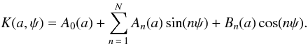 By minimizing particular terms, one can in principle find the centre, position angle, and axis ratio of the velocity field. Under the assumption that the velocity field is due to an axisymmetric thin disc, these correspond directly to the equivalent parameters for the galaxy (although one should bear in mind that, for example, with non-circular orbits the kinematic and isophotal major axes may not coincide; and for a geometrically thick system the axis ratio may not represent the inclination).
The correct choice of kinematic centre minimises A2 and B2 (which are also weakly dependent on ellipticity and PA) and to a lesser degree A1, A3, and B3 (see Krajnovic et al. 2006 for a more intuitive description of these parameters). The correct PA yields minimal values of A1, A3, and B3; correct ellipticity minimises B3. For a range of different ellipticities and PA, we place the kinematic centre at each pixel within a grid of 11 × 11 pixel centered on the AGN location and calculate the corresponding sum of A2 and B2. This results in a set of 2D maps of A2 + B2 for each combination of PA and ellipticity. The position of the minimum of each map then yields the best-fitting kinematic centre for that specific combination of PA and ellipticity. If the best-fit to the kinematic centre is the same for different values of ellipticity and PA (i.e. a unique best estimate for the kinematic centre exists), we then proceed to determine A1 and A3 at this kinematic centre for a range of different position angles, taking as the best estimate of the PA that value which results in A1 + A3 being minimal. Finally, the ellipticity is found by analogously minimising the B3 coefficient.
With this method we are able to find a unique solution for all three parameters for the southern nucleus. But it fails for the northern nucleus where the best estimates for kinematic centre and position angle are interdependent: the minima for A2 + B2 (determining the kinematic centre) lie on an arc with the exact position of the kinematic centre dependent on the choice of position angle. The only way out of this impasse is to make additional assumptions, and so we arrive at a “best-fit” by assuming the velocity field to have the same PA as the major axis of the continuum emission. We note that the PA of the continuum emission is independent of the extinction correction, because the extinction and continuum maps have the same PA. Figures 10 and 11 show the observed velocity field, the model, and the residuals for 2 cases in each nucleus: when the best-fitting centre derived from the kinemetry is used, and when the centre is fixed at the location of the black hole.
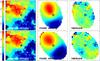 |
Fig. 10 Northern Nucleus: comparison of kinemetry models for 2 different PAs and kinematic centres. It should be noted that the rotation curves do not differ significantly for the two different positions of the kinematic centre. Black circles indicate black hole positions; black stars represent the kinematic centre; the dashed white line traces the major axis of rotation. Left to right: velocity map, model, and residuals. First row: best-fitting kinematic centre from kinemetry analysis. The average residuals per pixel are 33.5 km s-1. Second row: kinematic centre fixed at the position of the AGN. The average residuals per pixel are 35.3 km s-1. Image size is 820 × 720 pc. |
In the northern nucleus, the location of the derived kinematic centre is reasonably consistent with the black hole location, differing by only 0.12″. Since the average residuals per pixel are 33.5 km s-1 and 35.3 km s-1 for these two cases respectively, they can be considered statistically indistinguishable. We conclude that in the northern nucleus, we can confirm that the black hole is located at the kinematic centre of the stellar rotation.
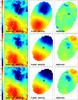 |
Fig. 11 Southern Nucleus: comparison of kinemetry models for different PAs and kinematic centres. It should be noted that the rotation curves do not differ significantly for the two different positions of the kinematic centre. Black circles indicate black hole positions; black stars represent the kinematic centre; the dashed white line traces the major axis of rotation. Left to right: velocity map, model, and residuals. First row: best-fitting kinematic centre from kinemetry analysis. Average residuals per pixel are 28.2 km s-1. Second row: kinematic centre fixed at the position of the AGN; average residuals per pixel are 45.9 km s-1. Third row: kinematic centre fixed at position of the AGN and performing fit only to southern half of nucleus. Average residuals per pixel over southern half are 21.1 km s-1. Image size is 600 × 840 pc. |
For the southern nucleus, the difference is more significant. The separation between the best-fitting centre and the AGN location is 0.22″. The mean residuals are 28.2 km s-1 (best-fit) and 45.9 km s-1 (AGN position). This can be understood with reference to the dispersion map in Fig. 4 and the extinction map in Fig. 9. The region to the northwest of the AGN in the southern nucleus exhibits both anomalously high dispersion and extinction – features that are to be expected in a merger system. It is therefore not clear whether the velocity field in this region is really tracing the rotation of the progenitor, or something more complex. Inspection of the residuals in Fig. 11 suggests the latter, an issue that we discuss in more detail in Sect. 6. Our conclusion for the southern nucleus is that the centre we derive from the velocity field is biased by perturbed kinematics on the northern side of the nucleus.
In both nuclei, for further analyses we therefore adopt the black hole locations of Max et al. (2007) as identifying the kinematic centres of the nuclei, and make use of the rotation curves, dispersion, and luminosity profiles centered at these positions. We derive axis ratios of 0.70 ± 0.02 and 0.65 ± 0.02 and PAs of 229° ± 2° and 329° ± 2° (measured east of north, PA pointing from receding to approaching velocities) for the northern and southern nuclei, respectively. We interpret the axis ratios in terms of an inclination for a flat system, noting that this may be an overestimate since the nuclei are likely to be thick. The impact is that we may also overestimate the intrinsic velocity.
6. Stellar kinematics between the nuclei
NGC 6240 is known to exhibit an exceptionally large stellar velocity dispersion between the nuclei (Lester & Gaffney 1994; Doyon et al. 1994; Tecza et al. 2000). In Fig. 4 we present a detailed 2D dispersion map which shows that the region with the highest (>300 km s-1) dispersion is fairly localised, and lies across the northern side of the southern nucleus. The localised nature of this region, together with poor signal-to-noise, most likely explain why Genzel et al. (2001) and Dasyra et al. (2006b) cite a significantly lower maximal dispersion, as it can easily be missed by slit measurements.
This high dispersion cannot be associated with the established stellar population in the southern nucleus because the high velocity (~500 km s-1 at 500 pc) implies a dynamical timescale of tdyn ~ 5 Myr. Any asymmetry in the dispersion of a stellar population orbiting the southern nucleus would be dispersed within this timescale. An alternative explanation is that this represents a region where emission from stars that have been formed recently as a result of the interaction is superimposed on the light from the nucleus. As the stellar kinematics are derived from absorption lines, a superposition of two populations at different line-of-sight velocities would lead to an overestimate of the dispersion: the line resulting from such a superposition would appear broader than the intrinsic line widths of each of its constituent lines. Fitting the resulting line profile with a single kinematic component would lead to a significant over-estimate of the disperion. Support for this explanation is lent by Ohyama et al. (2003). Based on a study of the morphology and kinematics of the warm and cold gas, they argued that clouds along the line of sight to the northern half of the southern nucleus were being crushed in the interaction. In this scenario, if the cloud crushing leads to star formation, there would indeed be two superimposed populations at this location. This is supported by Spitzer observations of the Antennae galaxies, which show that the largest energy output, and thus a high rate of star formation, occurs in the overlap region between the two galaxies’ nuclei (Brandl et al. 2009).
Although rather speculative, in the following discussion we consider whether this scenario can in principle account for both the increased dispersion and irregularities in the velocity in the northern half of the southern nucleus. Our aim is to use a very simple toy model to test the basic validity of the hypothesis by reproducing the characteristic features of the data; we do not attempt to match them exactly, nor to constrain the numerous parameters that would be required to do so.
We construct a two-population model as follows: the disc population is represented by a disc with the kinematic centre at the position of the AGN. PA, inclination, and velocity curve are found via a minimisation such as best to match the observed velocity field in the southern half. The dispersion is adopted from the radial dispersion curve derived from the southern half. We then subtract the disc velocity field from the observed velocity field in the northern half, and take this to be the velocity field of the second stellar population (thus ensuring that the observed velocity field is reproduced as closely as possible). In order to derive the resulting dispersion, we combine the two populations at each pixel by adding two Gaussians, with their centres corresponding to velocity and FWHM corresponding to dispersion (resembling the superposition of two absorption or emission lines). The resulting velocity field of the combination of both populations is then extracted by fitting a Gaussian to the result (resembling the method through which stellar kinematics are derived). As can be seen in Fig. 12, the model, whilst not matching the observations exactly, does reproduce the characteristic features of the data, displaying locally significantly increased velocity dispersions. The fact that the dispersion map is not reproduced exactly is due to the fact that we intentionally kept the model simple, assuming spatially constant, equal weightings and line FWHMs. We emphasise that the purpose of this exercise is simply to show that it is in principle possible to account for the locally significantly increased inferred dispersion through the effect of fitting a single velocity and dispersion to an absorption feature to which two stellar populations at different relative velocities have contributed. Although our assumptions that the two populations have the same luminosity and dispersion are simplistic, this underlines the point that a significantly better fit could be achieved if these parameters were allowed to vary. However, we feel that pursuing this is unjustified given constraints available from the data.
The total extinction-corrected luminosity emitted by the internuclear area with σ ≥ 330 km s-1 is 8.5 × 10⁸ L⊙. If this can be attributed in roughly equal shares to the old stellar population and the newly formed stars, it would imply a stellar mass of ~108 M⊙ contained in the starburst population in this area. We speculate that this population may have originated from star formation associated with gas between the nuclei, perhaps in the tidal bridge or clump discussed in Sect. 8.
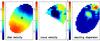 |
Fig. 12 Southern Nucleus: resulting apparent dispersion of the superposition of a “disc” population and a “cloud-crushing” population, both with velocity dispersions of 220 km s-1. Left to right: disc velocity field, cloud population velocity field, resulting apparent dispersion. Black circles indicate BH positions. The right panel shows that a simple “disc plus cloud” model can produce an increase in dispersion, characteristic of that observed (Fig. 4). This indicates that the high dispersion in the northern half of the southern nucleus may be an artifact due to the presence of two kinematically different stellar populations with similar luminosities. |
7. Jeans modelling, nuclear masses, and mass to light ratios
Knowledge of the rotational velocity field allows one to make simple Keplerian mass estimates. However, here the comparatively large velocity dispersions (generally σ/vrot > 1) necessitate a more sophisticated approach so as not to underestimate the actual mass. Two main avenues can be taken: Schwarzschild orbit superposition and Jeans modelling. The former proceeds by reproducing the velocity and dispersion maps from a large suite of stellar orbits calculated for a given potential, which is varied until a match to the observations is achieved. The latter employs the Jeans equations, derived by taking moments of the collisionless Boltzmann equation. For our data, Jeans modelling is better suited to recover the mass distribution, as the accuracy and resolution of our kinematic data is insufficient for Schwarzschild modelling.
A good overview of Jeans models can be found e.g. in Binney & Tremaine (2008). An important aspect of our approach is that we separate the gravitational potential Φ from the distribution of the stars, i.e. we allow for non-stellar mass. We assume isotropic velocity dispersion, which can be justified because the data do not allow us to say anything about the form of anisotropy, and this choice represents the least informative, and hence least constraining, option (Dejonghe 1986). Another issue is the shape of the stellar and total mass distribution. A discy system would be characterised by σ/vrot ≪ 1, and an oblate spheroidal system, in which the dispersion provides non-rotational pressure support thickening the disc, by a σ/vrot ≳ 1. Figure 4 shows that for both nuclei in NGC 6240 σ/vrot ~ 1, suggesting that the latter is the more physically realistic choice. However, this is non-trivial to implement (see for example van der Marel & van Dokkum 2007). Instead we make the simplifying assumption that both the stellar distribution and potential are spherically symmetric, which will allow us to capture the characteristics of the system. It also has the advantage of yielding an analytical solution.
In order to assess the uncertainties of our result due to the choice of mass distribution, we also ran a set of models assuming an axisymmetric thin disc with an isotropic pressure component; the enclosed masses found with this model, which can be considered to be at the other end of the range of physically plausible models, agreed with the results of the spherically symmetric models within a factor of less than two. Häring-Neumayer et al. (2006) model the gas kinematics of Cen A with three different Jeans models: an axisymmetric thin disc with and without pressure terms, and a spherically symmetric model. They find that the inferred black hole masses span less than an order of magnitude. Comparing their results with those of others, these authors find that, whilst favouring the pressure-supported thin disc model as the most physically plausible, the spherical Jeans model agrees best with the results from Schwarzschild orbit superposition modelling by Silge et al. (2005). The uncertainty of Jeans modelling results due to the unknown velocity dispersion anisotropy is more difficult to assess due to the degeneracy between the integrated mass and the anisotropy parameter β. Both Wolf et al. (2010) and Mamon & Boué (2010) attempt to quantify this (see Fig. 1 in Wolf et al. 2010; and Fig. 1 in Mamon & Boué 2010) in the case of mass measurements for the Carina dSph and DM haloes, respectively, finding that the range spanned by results for the integrated mass assuming extreme values of β are large at small physical radii, decreasing to less than a factor of two at radii comparable to or larger than the half-light radius. Since a spheroidal system like the one we modelled is unlikely to have extremely anisotropic velocity dispersions, and since also we are measuring mass at radii larger than the half-light radius, we can assume the factor of two derived by these authors to be an upper limit on the error due to our choice of β = 0. We thus estimate that the uncertainties introduced by the assumptions inherent in our modelling are unlikely to be larger than a factor of two.
Jeans modelling requires luminosity, rotational velocity, and velocity dispersion profiles as input. Since the region between the two nuclei is likely strongly perturbed, we measured azimuthally averaged profiles using only a 180° wedge in the outside halves (i.e. opposite the merger centre) of the galaxy, after subtracting the continuum associated with the recent starburst (assuming an intrinsic WBrγ of 22 Å, as measured at the knot of Brγ emission north-west of the northern nucleus, cf. Sect. 9) and correcting for extinction. To these we fitted a Sérsic function to the profiles, constraining it with the NIRC2 profile at >0.4″, and with the extinction-corrected SINFONI profile at <1.0″ (i.e. some overlap between the two profiles is included). As part of the fitting process, the model profile was convolved in 2D with the SINFONI PSF, to account for beam smearing at small scales. We then analytically deprojected these LOS luminosity profiles. The measured rotation curves and dispersion profiles need to be corrected for beam smearing and projection along the line of sight in order to recover the intrinsic kinematics. For this, we used the code described in Cresci et al. (2009).
With these inputs, we compute M(r). The total mass enclosed within the cut-off radius (250 pc and 320 pc for northern and southern nuclei, respectively) is found to be 2.5 × 10⁹ M⊙ and 1.3 × 10¹⁰ M⊙. This is comparable to that seen in the central few hundred parsecs of nearby AGN (Fig. 7, Davies et al. 2007). We also calculate a global K-band mass-to-light ratio by finding the multiplication factor that best matches the luminosity enclosed at radius r to M(r). Here, as in the rest of the paper, LK is taken to be the total luminosity in the 1.9–2.5 μm band in units of bolometric solar luminosity where 1 L⊙ = 3.8 × 1026 W (we note that a commonly used alternative is the definition via solar K-band lumnosity density, 2.15 × 1025 W μm-1). We obtain values of 5.0 M⊙/L⊙ and 1.9 M⊙/L⊙ for the northern and southern nuclei. Downes & Solomon (1998) find typical gas fractions of ~15% for local ULIRGs; in conjunction with these modelling results, this implies total stellar masses of 2.1 × 10⁹ M⊙ and 1.1 × 10¹⁰ M⊙, and stellar mass-to-light ratios of 4.3 M⊙/L⊙ and 1.6 M⊙/L⊙ for the northern and southern nuclei, respectively. We discuss the possible inferences from these results regarding the nature of the nuclei and the progenitors’ Hubble types in Sect. 10.
It is tempting to compare the mass enclosed in the innermost few parsecs to the expected black hole masses. One avenue to estimate the black hole masses is afforded by the X-ray luminosities. Vignati et al. (1999) measure a total absorption-corrected nuclear X-ray luminosity in the 2–10 keV range of 3.6 × 1044 erg s-1 with BeppoSAX. Komossa et al. (2003), using CHANDRA, find that the northern and southern nuclei have absorption-corrected 0.1–10 keV X-ray luminosities of 0.7 × 1042 erg s-1 and 1.9 × 1042 erg s-1, respectively. The discrepancy is most likely due to different absorption corrections (Komossa et al. (2003) derive NH ~ 1022 cm-2, Vignati et al. (1999) measure NH ≈ 2 × 1024 cm-2). Since Vignati et al. (1999) derive their absorption correction from a significantly larger wavelength range (up to 100 keV) we use their values for the following estimates. We convert the X-ray luminosity to monochromatic 5100 Å luminosity using the luminosity dependent αOX-relation (Steffen et al. 2006; Maiolino et al. 2007), and then convert to AGN bolometric luminosity adopting Lbol = 7νLν (5100 Å) (e.g. Netzer & Trakhtenbrot 2007). Dasyra et al. (2006b) calculate Eddington ratios for a sample of 34 ULIRGs, finding a median value of 0.37. With this value for Lbol/LEdd, we arrive at a combined black hole mass of 4 × 10⁸ M⊙. However, the uncertainty on this estimate is at least a factor of a few.
Alternatively estimates can be derived from the stellar velocity dispersions. Using the MBH-σ relation from Tremaine et al. (2002) and the stellar dispersions measured at the locations of the AGN (~200 km s-1 and ~220 km s-1 for the northern and southern nuclei, respectively) yields expected central black hole masses of 1.4 ± 0.4 × 10⁸ M⊙ and 2.0 ± 0.4 × 10⁸ M⊙ for the northern and southern nuclei, respectively. The uncertainties on black hole masses derived from the MBH-σ relation are also a factor of a few.
Finally, a measurement (with a rather smaller uncertainty) of MBH in the southern nucleus can been made using high resolution stellar kinematics. Resolving the gravitational sphere of influence of the black hole and modelling the kinematics, Medling et al. (in prep.) derive a preliminary mass of 2.0 ± 0.6 × 10⁹ M⊙.
Although the range of MBH above spans an order of magnitude, the very large uncertainties of the first 2 estimates means that all the estimates are formally consistent (within ~2σ). We therefore caution against over-interpretation.
8. Merger geometry and stage, and cold gas concentration
Starting from the assumption that the projected angular momenta of the nuclei are the true angular momenta, Tecza et al. (2000) proposed a merger geometry in which one of the nuclei is coplanar and prograde with the merger orbital plane, and the other is inclined with respect to the orbital plane (their Fig. 11). They further supported the notion of at least one of the galaxies being subject to a prograde encounter by noting that the formation of tidal tails such as those of NGC 6240 is favoured in prograde encounters. Here we would like to build onto and expand this discussion.
NGC 6240 indeed has long, well developed tidal tails, as can be seen in optical and HI data (Gerssen et al. 2004; Yun & Hibbard 2001), covering a projected size of ~45 kpc from north to south, about half that of the Antennae. In the HST images, a continuous dust distribution across the centre strongly suggests that what we are seeing is an extended, well developed single tail curving in front of the system, rather than a series of disconnected shorter features. However, NGC 6240’s tails are not as dense or long as those of e.g. the Antennae. What can we derive from this with regard to the merger geometry? It is generally known that in merger simulations, the more coplanar/prograde, and thus “resonant”, an encounter is, the stronger the resulting tidal tails are. It is quite clear however, from looking at the relative orientation of the rotation axes of the nuclei, that NGC 6240 cannot be a perfectly coplanar merger. But a merger must not be exactly coplanar and prograde in order to produce tidal tails – an example of this is NGC 7252, which has tidal tails akin to those of NGC 6240. NGC 7252’s tidal features were successfully reproduced through N-body simulations by Hibbard & Mihos (1995); their simulation had one of the progenitors on a coplanar, prograde encounter, but the other galaxy at an inclination of ~45 degrees to the orbital plane – this illustrates that there is a non-negligible merger parameter space around “coplanar/prograde” which will also result in pronounced tidal tails. Therefore, whilst not pinning down the merger geometry exactly, the existence of such long and well developed tidal tails is convincing evidence that the merger geometry must be within a reasonable parameter space around prograde/coplanar. The stellar kinematics at first sight seem to disagree with this, giving the appearance that the nuclei are counter-rotating. However, co-rotating nuclei would also look like this if one nucleus is inclined behind the plane of the sky, and the other in front. Thus the stellar kinematics are consistent with the view that NGC 6240 is not too far from being a prograde merger. That the nuclei are clearly not exactly aligned could be the reason for the additional shorter tails that make the system look rather messy.
We therefore conclude that NGC 6240’s merger geometry most likely tends towards coplanar/prograde, and in this sense is perhaps quite similar to the geometry proposed for NGC 7252 by Hibbard & Mihos (1995).
It is more difficult to deduce the stage of merging the two galaxies comprising NGC 6240 are currently in – we cannot pin down their merger geometry exactly, as discussed above, and neither do we know the 3D relative velocities of the two nuclei, so we cannot calculate whether the two nuclei will merge immediately or separate again before eventually coalescing. We know that they must certainly have already experienced their first close encounter, since tidal tails only form after the first strong gravitational interaction of the two galaxies. This is also supported by the high luminosity of the system, because elevated levels of star formation also are only expected after the first encounter leads to collision and compression of gas complexes. And the fact that the two nuclei are still separated by about a kpc in projection indicates that the system is not yet at the “final coalescence” phase.
The observed peak of the gas emission between the nuclei (Fig. 5), which Tacconi et al. (1999) found to display a velocity gradient and interpreted as due to a self-gravitating gas disc located in between the nuclei, is puzzling, since from merger simulations this is generally not expected to occur. We could be seeing a collapsed gas clump in a tidal arm – such features are found to occur quite often in simulations of merging galaxies above a certain gas fraction (Wetzstein et al. 2007; Bournaud et al. 2008), and are also seen in observations (Knierman et al. 2003). An alternative, and perhaps more likely, interpretation of this gas concentration is a tidal bridge connecting the two nuclei that is viewed in projection. Such tidal bridges are often seen in merger simulations. However, simulations have never yielded a system in which the total gas mass is dominated by that between the nuclei. And although bridges are produced most strongly in a perfectly prograde coplanar encounter (which, as discussed above, is inconsistent with our observations), as one deviates from a prograde coplanar geometry the strength of the bridge decreases.
An alternative, although somewhat rarer, way to drive a significant gas mass away from the nuclei is a direct interaction (i.e. low impact parameter), in which the ISM of the progenitors collides. The best example of this is UGC 12914/5 (the Taffy Galaxies; Braine et al. 2003), in which about 25% of the CO emission originates between the nuclei. In this system, the progenitors collided at about 600 km s-1. Braine et al. (2003) argued that while this would have ionised the gas, the cooling time is short enough that H2 could reform while the discs are still passing through each other. From the ratio of 12CO to 13CO these authors found that the optical depth of CO in the bridge was far less than on the nuclei. Combined with the effect of increased CO abundance due to grain destruction, this led them to suggest that the actual mass of molecular gas may be rather less than implied by the CO luminosity, perhaps only ~6% of the total gas mass. Since direct collisions such as these tend to create ring galaxies (or in the case of the Taffy Galaxies, an incomplete ring or hook), this scenario seems unlikely for NGC 6240.
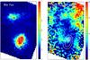 |
Fig. 13 Left: map of Brγ flux (units given in 10-16 W m-2 μm). Right: map of WBrγ (units given in Å). White contours tracing the K-band stellar continuum, and black circles denoting the black hole locations are overdrawn on both maps. Although the most intense Brγ emission is on the nuclei, the equivalent width here is lowest, suggesting that the K-band light is dominated by an older stellar population. We note that in Sect. 4 we showed that dilution by hot dust emission associated with the AGN cannot play a role in reducing WBrγ. |
In NGC 6240, the CO map indicates that CO luminosity is dominated by that between the nuclei. We must therefore consider physical effects that could significantly affect the flux-to-mass conversion factor between the two regions. It is already known that sub-thermal emission from non-virialised clouds can radically modify the CO-to-H2 conversion factor, as shown in Fig. 10 of Tacconi et al. (2008). Such an effect could easily boost the emission from gas in a drawn-out, thin and diffuse gas bridge compared to denser material around the nuclei. And it is supported by other observations: a comparison of the CO line emission (Fig. 5) with the 1.315 mm continuum measured by Tacconi et al. (1999, their Fig. 3, left panel) shows that the dust, as traced by the mm continuum, is concentrated on the nuclei rather than following the CO line emission. Furthermore, in a detailed analysis of various CO transitions, Greve et al. (2009) were unable to find a single set of average H2 conditions that comes close to reproducing the observed line ratios. A second important issue is the impact of X-ray irradiation on the CO abundance around the nuclei, since the AGN are quite luminous. Lutz et al. (2003) argue that as little as 25–50% of Lbol is due to the AGN. If we take the lower end of this range, and distribute it equally between the two AGN, we find each radiates at L ~ 3 × 1044 erg s-1. We also adopt a column of 2 × 1024 cm-2 (Vignati et al. 1999) and assume a gas density of 105 cm-3. Under these conditions, hard X-rays from the AGN will cause sufficient ionisation to reduce the CO abundance an order of magnitude below its typical value of 10-4 out to a radius of 250 pc (see Boger & Sternberg 2005; and Davies & Sternberg, in prep.). Thus, even if there is significant gas mass around the nuclei (as the models imply), one would expect rather little CO emission. That these effects will conspire to make the CO luminosity distribution look rather different to the molecular gas mass distribution should be borne in mind.
9. Scale of starburst and star formation history
While Tecza et al. (2000) concluded that the nuclei were the progenitor bulges, they did not quantify how much of the K-band luminosity arises in the recent starburst and how much is due to the progenitor bulges themselves. Our data enable us to resolve this issue. Our method is to measure an average value for WBrγ away from the nucleus where dilution from the bulge is small, and assert that this is representative of the whole starburst. The fundamental assumption is that, integrated over a sufficiently large aperture, we are summing a fair cross-section of star clusters and hence probing the average star formation properties. This minimises the impact of the stochastic nature of individual clusters. We have therefore chosen a region containing a high density of clusters, and measured WBrγ in a 0.8″ aperture corresponding to 400 pc so that many clusters are included. Such a region lies about 1″ to the west of the northern nucleus (Pollack et al. 2007), sufficiently far that the K-band continuum from the nucleus is very faint. Figure 13 shows that, despite the Brγ flux being higher on the nuclei, both here (and also in other off-nuclear regions) WBrγ = 22 ± 6 Å. We use it to obtain the fractional contribution of the young stellar population in 1″ diameter apertures centred on the nuclei, by dividing the measured WBrγ by this intrinsic value. We then find the K-band luminosity emitted by the starburst population to be 3.6 × 10⁸ L⊙ (northern nucleus) and 1.3 × 10⁹L⊙ (southern nucleus), implying LK,young/LK,total to be 0.36 (northern nucleus) and 0.32 (southern nucleus) – i.e. only about 1/3 of the total K-band luminosity of the nuclei is due to recent star formation.
Characteristics of starburst populations.
This implies that the K-band luminosity of the nuclei is dominated by a population of stars older than 20 Myr. An important question is whether this is consistent with claims that one needs supergiant templates in order to match the CO bandhead depth (Lester et al. 1988; Sugai et al. 1997; Tecza et al. 2000). In the following, we show that basing conclusions about the dominant stellar population on a fit to a single template is very uncertain. The tables in Origlia et al. (1993) and Förster Schreiber (2000) show that the equivalent widths of the CO bandheads vary considerably between individual stars; and it is also well known that higher metallicity populations have deeper bandheads because the K-band continuum is dominated by cooler stars. The templates found by Tecza et al. (2000) and Sugai et al. (1997) to provide the best fit to the K-band absorption features are of K4.5 Ib and K2.5 Ib stars, respectively: i.e. specifically K type sub-luminous supergiants. Both authors infer from this that the dominant stellar population is late type supergiants. Tecza et al. (2000) go on to conclude that these were produced as a result of a burst of star formation that lasted for 5 Myr and occurred ~20 Myr ago. We have examined the Tecza et al. (2000) starburst scenario in detail using the population synthesis code STARS, and found that it would lead to ~60% of the K-band luminosity being due to M supergiants (cooler than 4000 K) and only ~3% due to K supergiants (temperatures 4000–4600 K). Thus the scenario of a ~20 Myr old starburst leads to two apparent contradictions: How can M supergiants dominate the luminosity and yet have absorption features too deep to match the spectrum? And how can K supergiants provide a good match to the spectrum and yet contribute only an insignificant fraction of the luminosity? The resolution is simply that the galaxy spectrum consists of many different types of stars, and a single template can at best be characteristic of the sum of all these. The important conclusion here is that while the composite spectrum is best matched by a supergiant template, other types of stars still make up a significant fraction of the near-infrared continuum.
In addition to the current scale of the starburst, another key point of interest are the past and future star formation rates. Di Matteo et al. (2007, 2008) and Cox et al. (2006, 2008) offer a large sample of medium-resolution simulations comprehensively covering a wide range of gas fractions, merger geometries, and mass ratios, as well as employing different codes. Their synthesised results regarding the qualitative evolution of the star formation during a merger are that nearly all encounters are marked by at least two peaks in the star formation rate; one at the first encounter, and one upon final coalescence. However, the relative strength of the two peaks differs, depending on the merger geometry; but on average the second peak is stronger (Di Matteo et al. 2007, 2008). This is particularly evident for mergers that tend towards coplanar/prograde geometries, as appears to be the case for NGC 6240.
The aforementioned simulations were carried out at medium resolution, and thus one might ask whether their results would change when going to higher resolution simulations resolving the multiphase ISM. However, as Bournaud et al. (2008) and Teyssier et al. (2010) show, the qualitative evolution of the star formation rate during a merger remains largely unchanged, the only significant difference is that star formation proceeds much more effectively, resulting in predicted star formation rates a factor of up to ten times larger than those predicted by lower-resolution simulations (Teyssier et al. 2010).
We therefore conclude that NGC 6240, being between first encounter and final coalescence, most likely experienced its first peak in star formation rate in the recent past (triggered by the first encounter); has currently elevated levels of star formation compared to a quiescent galaxy; and will experience another, likely stronger, peak in star formation rate in the near future when the galaxies coalesce. This is supported by the observed Brγ emission, which indicates that star formation must currently still be on-going, and by measurements of cluster ages (Pollack et al. 2007) which are found to be typically very young – in a population of clusters with a range of ages, it is the brighter ones that are more easily detected, and because clusters fade quickly, these will also inevitably be younger. We furthermore note that since NGC 6240 is already just below the canonical ULIRG threshold of LIR ≳ 1012 L⊙, it is safe to predict that it will breach this threshold once the final starburst is triggered, and will become a bona fide ULIRG.
In order to be able to make more quantitative analyses, we use STARS to calculate a range of observables from two star formation histories, which both display the generic features discussed above; an initial peak at first encounter followed by a gradual rise or plateau, and a final intense burst. One of these simulations is selected from a set of simulations intended to reproduce the properties of the Antennae galaxies (Karl et al. 2008, 2010), and the other one from the library of Johansson et al. (2009). Neither are coplanar/prograde, although they tend towards it, and both produce well-developed tidal tails during the interaction. The rationale of using star formation histories from two different simulations is to provide an estimate of the uncertainties introduced by the quantitative differences introduced by the exact simulation details. Since we only know that NGC 6240 must be between first encounter and final coalescence, we use the full range of simulated properties between these two points, as well as our measurement and associated uncertainties of WBrγ, as constraints to derive the uncertainties in the star formation properties.
In Table 2, we have used these star formation histories to calculate the mass of young stars formed in both scenarios, as well as the current star formation and supernova rates. To do so, we have applied a scaling so that the K-band luminosity matches that observed for each nucleus, under the assumption that the evolution of the central SFR mirrors that of the global SFR. The table shows that quantitatively the results for the two different star formation histories do not differ greatly – in fact, the variation within each scenario over the possible time range is larger than the variation between the averages of the two cases.
One conclusion is that the bolometric luminosity of the starburst from the two nuclei together is only 20–30% of the system’s total. This follows in the same direction as Lutz et al. (2003) that the recent starburst only contributes part of the total luminosity. We estimate a somewhat lower fraction than Lutz et al. (2003), who constrain starburst contribution to be 50 to 70%, possibly due to the fact that we are looking at the central region whereas they investigated the global luminosities.
An important concern is that our results appear to be inconsistent with those of Beswick et al. (2001) who find, based on the 1.4 GHz continuum, significantly larger star formation and supernova rates of 83.1 M⊙ yr-1 and 1.33 yr-1. We argue that this is due to the different star formation histories adopted. We show that this can have a major impact on interpretation of the data, and that accounting for it makes the radio continuum data consistent with our results.
We first address a minor correction, specifically a ~10% increase in radio flux due to the larger aperture used by Beswick et al. (2001), which included a substantial flux contribution from an off-nuclear source not included in our apertures (“N2” in their nomenclature, see their Fig. 2). A larger correction may be needed by analogy to Arp 220 for which Rovilos et al. (2005) examined the 18-cm lightcurves of the supernovae. They found the type IIn RSNe model insufficient and arrived at a supernova rate that was a factor of ~3 smaller than the ~2 yr-1 often quoted. A similar correction may be applicable to the rates inferred from radio measurements for NGC 6240. This may be related to the third issue, which concerns the star formation history. The formulae used by Beswick et al. (2001) to convert 1.4 GHz luminosity to star formation and supernova rates (based on work by Condon & Yin 1990; Condon 1992; Cram 1998) were derived empirically based on measurements of normal disc galaxies for which a constant star formation rate is characteristic. This implicit constant star formation rate is very different to the increasing star formation rate found in merger simulations. We show below that this can make as much as a factor of three difference in the star formation and supernova rates that are derived from observables.
We use STARS to estimate the star formation rate from a given K-band luminosity for three different star formation histories. First, following Beswick et al. (2001), we adopt continuous star formation for a duration of 20 Myr, corresponding to that estimated by Tecza et al. (2000), Pasquali et al. (2003), Pollack et al. (2007) for the most recent star burst. In order to reach LK = 1.7 × 10⁹ L⊙, corresponding to the total measured for the starburst population, we require a constant SFR of 25 M⊙ yr-1. On the other hand, for the recently increasing star formation rate typical of the merger scenarios, we find star formation rates of ~10 M⊙ yr-1. Thus we find a factor ~2.5 difference in the SFR required to reach the same K-band luminosity, depending on the star formation history. We can estimate the supernova rates in a similar way: for 20 Myr of continuous star formation at 25 M⊙ yr-1, we calculate a supernova rate of 0.3 yr-1. In contrast, for our merger scenarios, we find supernova rates of ~0.13 yr-1. Thus, much of the discrepancy between our supernova rate and the (corrected) value from Beswick et al. (2001) is due to the different star formation histories adopted.
This illustrates an important caveat: the choice of star formation history can have a far-reaching impact on the interpretation of the observables. We note that the very similar derived stellar population parameters for our two different merger star formation histories indicate that, for mergers, using a “characteristic” star formation history (i.e. an initial peak at first encounter followed by a gradual rise or plateau, and a final intense burst) will yield much more reliable quantities than either instantaneous or continuous star formation models.
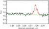 |
Fig. 14 Spectrum of the region to the northwest where the WBrγ is not diluted by continuum emission from the progenitors, integrated over an 0.8″ diameter aperture. The flux is in units of 10-16 W m-2 μm-1. The measured WBrγ is 22 ± 6 Å. |
Properties of the nuclei.
10. Stellar populations of NGC 6240
Did the progenitors have bulges?
The existence or otherwise of bulges (where “bulge” here includes both pseudobulges and classical bulges) in the galaxies undergoing a merger has a profound impact on the star formation (Mihos & Hernquist 1996). Springel et al. (2005) show in their Fig. 15 that in a major merger of discs (gas fraction 10%) without bulges, the first encounter already triggers an episode of enhanced star formation that lasts for 300–400 Myr. The second encounter triggers a more intense, but also somewhat shorter (~50 Myr), starburst 800–900 Myr later. In a simulation that included a bulge and a central black hole, there was almost no perceptible change in the star formation rate at the first encounter. This remained constant at ~5–10% of the peak star formation rate until the second encounter, when the starburst is triggered and the peak star formation rate was achieved. Because there had been no earlier phase of enhanced star formation, this starburst is more intense than it would be without a bulge. Which of these two different scenarios holds true for NGC 6240?
The evidence overwhelmingly points towards the progenitors having had a prominent bulge component. First, the majority of massive spirals at low redshifts have bulges, although at z ≳ 2 the situation may well be different as bulges may not yet have had time to grow (Genzel et al. 2008). Second, we know that both nuclei host an AGN and therefore harbour a supermassive black hole. The implication of the MBH-σ ∗ relation is therefore that the progenitors must have had bulges. Using estimates of the black hole masses based on the AGN luminosity and our measured stellar dispersion (Sect. 7) in conjunction with the empirical correlation between MBH and bulge mass (Häring & Rix 2004) yields associated bulge masses of 8.7 × 10¹⁰ M⊙ and 1.2 × 10¹¹ M⊙ for the northern and southern nuclei respectively, an order of magnitude larger than their dynamical masses. However, due to their transformational impact on both black hole and host galaxy, it is uncertain whether such scaling relations can be expected to hold during on-going mergers. An argument favouring the existence of bulges in the progenitors stems from the merger simulation: the galaxies in our simulation had bulges, and the good match to the observed WBrγ suggests that the star formation history is reasonable. As Springel et al. (2005) and Di Matteo et al. (2007, 2008) show, bulgeless mergers have markedly different star formation histories, with the first encounter producing the most potent burst of star formation (it should furthermore be noted that in higher-resolution simulations, the starburst triggered by the final coalescence occurs somewhat earlier; cf. Teyssier et al. 2010.). Thus, at the current phase, we would expect to see significantly lower WBrγ if the first encounter had indeed triggered the more powerful star formation event.
Are the nuclei the progenitors’ bulges?
Are the nuclei we see (remnants of) the progenitor galaxies’ bulges, did they originate only in the first encounter a few 100 Myr ago, or is the rotation we see the signature of stellar discs? The latter is unlikely, since the high dispersion clearly indicates a thickened structure, and nuclear stellar discs in contrast are often accompanied by sigma-drops (Peletier et al. 2007). Tecza et al. (2000) proposed the first, based on an estimate of the global mass-to-light ratio of the nuclei. Our high spatial resolution data allow us to explore this in more detail using not only the mass and luminosity, but also the effective radius and kinematics, and our knowledge of the stellar populations.
Table 3 quantifies the kinematics, luminosities, masses, and sizes of the two nuclei. How do these compare with the characteristics expected of a bulge? An argument in favour of the nuclei being bulges is supplied by estimates of the mass-to-light ratio of the non-starburst stellar population: correcting the global stellar mass-to-light ratios (Sect. 7, assuming a gas fraction of ~15%) for the starburst contribution (Table 2), we find that the non-starburst nuclear populations must have mass-to-light ratios of ~5.2 M⊙/L⊙ (northern nucleus) and 1.8 M⊙/L⊙ (southern nucleus) – noting that the associated uncertainties are estimated to be about a factor of two. If the nuclei only formed after the first encounter (~560 Myr ago in the “Antennae” scenario), they should have a M/LK of at most 2 M⊙/L⊙, whereas a several Gyr old stellar population has a M/LK of ~6–10 M⊙/L⊙ (e.g. Fig. 4 in Davies et al. 2007). This, as well as the small relative contributions of the starburst population to the nuclear masses and luminosities, indicates that a substantial fraction of the nuclei consists of stars predating the beginning of the merger.
NGC 6240 has often been cited as having anomalously high stellar dispersion. However, excluding the region towards the northern half of the southern nucleus which we discuss in Sect. 6, the dispersions typical for the nuclei are ~200 km s-1. These are not unusual for late-type bulges, as Fig. 18 in Kormendy & Kennicutt (2004) shows. Placing the two nuclei on the ϵ vs. vmax/σ diagram of Kormendy & Kennicutt (2004) (their Fig. 17), it appears that the northern nucleus lies comfortably within the region typical for late-type pseudobulges, whereas the southern nucleus would represent a somewhat more extreme case, having a higher vmax/σ than other galaxies. In both cases, however, the kinematics strongly support the case for a disc-like, secularly-grown pseudobulge rather than a merger-formed classical bulge. The Sérsic indices are rather typical of classical bulges, but we caution that the luminosity profiles are disturbed and influenced by recent star formation, and hence the values derived from the Sérsic fits should be treated with caution. For the same reason, we prefer to measure the sizes from the extents to which rotation can be seen (indicating the extent to which the nuclei dominate the light distribution), rather than the effective radii obtained from the Sérsic fits; this gives radii of 265 pc and 290 pc for the northern and southern nuclei, respectively (as opposed to 490 pc and 180 pc based on the Sérsic fits). This places them at the lower end but within the range given by Moriondo et al. (1999) who measure the bulge radii for 40 spiral galaxies and find values ranging from 230 pc to 1.93 kpc with an average of 650 pc. The same authors also look at the bulge masses, where they find values from 1.4 × 10⁹ M⊙ to 1.8 × 10¹¹ M⊙ with an average of 2.5 × 10¹⁰ M⊙. Our analysis (Sect. 7) yields masses of 2.5 × 10⁹ M⊙ and 1.9 × 10¹⁰ M⊙, again at the lower end but within the range found by Moriondo et al. (1999).
Would we expect the bulges to survive to this merger state? Comparatively little is known about the evolution of galaxy bulges during mergers. Observationally, Agüero et al. (2001) report velocity dispersions of 217 km s-1 and 280 km s-1 in the two nuclei of the merger system AM 2049-691, and Shier et al. (1998) investigate 11 multiple-nucleus merging objects and find nucleus sizes between 200 and 1600 pc (on average 600 pc), velocity dispersions of 66–151 km s-1 (excluding NGC 6240, which was also sampled) with an average of 109 km s-1. However, these were to a large part galaxies in earlier merger stages. Hernquist (1993) simulates the merger of two spiral galaxies with bulges. His model suggests that the bulges remain very nearly intact until final coalescence. The spin (rotational velocity) is reported to remain nearly constant throughout the simulated merger.
In light of this and the fact that the nuclei are found towards the lower end of the range of masses and sizes found for a large sample of spiral galaxy bulges, we conjecture that the nuclei are indeed the progenitor galaxies’ bulges, most likely pseudo-bulges, that have had their outer, less tightly bound layers stripped off during the merger, leading to the sub-average sizes. Dispersion may have increased due to “heating” during the interaction by gravitational impulse, and a gravitational potential deepened by influx of gas into the central region. Since the progenitors did not only have a prominent bulge component, but must also have had substantial discs in order to allow such pronounced tidal features as we observe to develop, the progenitors were most likely of Hubble type Sa/Sb.
11. Conclusions
We present new adaptive optics integral field spectroscopy near-IR data and CO(2–1) interferometric line observations of the nearby merger system NGC 6240. Our main conclusions are:
-
The Calzetti et al. (2000)reddening law provides the best fit to photometric data pointsspanning 0.45 μm to 2.22 μm. The spatially resolved extinction is generally moderate, with AK ~ 2–4.
-
The locations of the stellar kinematic centres are consistent with the black hole locations proposed by Max et al. (2007). However, an additional stellar population along the line of sight may be perturbing the velocity field of the southern nucleus and causing the higher dispersion across the northern side.
-
Jeans modelling of the stellar kinematics, assuming spherical symmetry and isotropic dispersion, gives M = 2.5 × 10⁹ M⊙ and M/LK = 5.0M⊙/L⊙ for the northern nucleus (out to 250 pc), and M = 1.9 × 10¹⁰M⊙ and M/LK = 5.0M⊙/L⊙ for the southern nucleus (out to 320 pc).
-
The presence of tidal arms, and the still-separated nuclei indicate that NGC 6240 must be between first encounter and final coalescence. The stellar velocity field, and strength and prominence of the tidal arms indicate that this system is not perfectly, but reasonably close to prograde coplanar.
-
Although simulations can produce significant projected gas mass between the nuclei, these are never as prominent as the observed concentration in CO luminosity. In order to explain this, additional physical effects such as spatial differences in CO-to-H2 conversion factor or CO abundance are needed.
-
Star formation histories from numerical simulations display generic features. Using these in combination with our constraints on the merger stage and measurements of WBrγ, we calculate the properties of the young starburst population. We find that recent star formation accounts for only about 1/3 of the total K-band luminosity. Thus the stellar luminosity is dominated by stars predating the merger.
-
Whereas the differences between the starburst properties inferred from different merger star formation histories appropriate to NGC 6240 are markedly small, adopting a constant star formation rate yields very different results (such as a actor 3 change in the derived SFR). We conclude that, when characterising the star formation properties of a merger, a “generic” merger star formation history should be adopted in preference to either instantaneous or constant star formation histories.
-
After accounting for the recent star formation, the mass-to-light ratios of the remaining stellar population are 5.2 M⊙/L⊙ and 1.8 M⊙/L⊙ for the northern and southern nuclei respectively. This implies that a population of stars older than ~1 Gyr contributes the majority of the nuclear stellar masses and luminosities. Combined with the measured size and V/σ, as well as results from the simulations, it implies that the two nuclei are the remnants of the bulges of the progenitor galaxies.
Acknowledgments
The authors would like to thank the anonymous referee for a thorough and thoughtful reading of the manuscript, which helped to clarify and improve the paper. H. Engel would like to thank Scott Tremaine and Payel Das for interesting and helpful discussions on Jeans modelling. The numerical simulations were performed on the local SGI-Altix 3700 Bx2, which was partly funded by the Cluster of Excellence: “Origin and Structure of the Universe”. Some of the data presented here were obtained at the W. M. Keck Observatory, which is operated as a scientific partnership among the California Institute of Technology, the University of California, and NASA. This work was supported in part by the NSF Science and Technology Center for Adaptive Optics, managed by the University of California at Santa Cruz (under cooperative agreement no. AST-9876783).
References
- Abuter, R., Schreiber, J., Eisenhauer, F., et al. 2006, NewAR, 50, 398 [CrossRef] [Google Scholar]
- Agüero, E. L., Díaz, R. J., & Paolantonio, S. 2001, PASP, 113, 1515 [NASA ADS] [CrossRef] [Google Scholar]
- Alonso-Herrero, A., Rieke, G. H., Rieke, M. J., et al. 2006, ApJ, 650, 835 [NASA ADS] [CrossRef] [Google Scholar]
- Armus, L., Heckman, T. M., & Miley, G. K. 1990, ApJ, 364, 471 [NASA ADS] [CrossRef] [EDP Sciences] [Google Scholar]
- Armus, L., Bernard-Salas, J., Spoon, H. W. W., et al. 2006, ApJ, 640, 204 [NASA ADS] [CrossRef] [Google Scholar]
- Barnes, J. 2002, MNRAS, 333, 481 [NASA ADS] [CrossRef] [Google Scholar]
- Beswick, R., Pedlar, A., Mundell, C., & Gallimore, J. 2001, MNRAS, 325, 151 [NASA ADS] [CrossRef] [Google Scholar]
- Binney, J., & Tremaine, S. 1987, Galactic Dynamics (Princeton: Princeton University Press) [Google Scholar]
- Binney, J., & Tremaine, S. 2008, Galactic Dynamics, 2nd edn. (Princeton: Princeton University Press) [Google Scholar]
- Bland-Hawthorn, J., Wilson, A. S., & Tully, R. B. 1991, ApJ, 371, L19 [NASA ADS] [CrossRef] [Google Scholar]
- Boger, G., & Sternberg, A. 2005, ApJ, 632, 302 [NASA ADS] [CrossRef] [Google Scholar]
- Bonacini, C., et al. 2006, in Advances in Adaptive Optics II, ed. B. Ellerbroek, & C. D. Bonaccini, Proc. SPIE, 6272, 627207 [Google Scholar]
- Bondi, H., & Hoyle, F. 1944, MNRAS, 104, 273 [NASA ADS] [CrossRef] [Google Scholar]
- Bonnet, H., Abuter, R., Baker, A., et al. 2004, The ESO Messenger, 117, 17 [Google Scholar]
- Bournaud, F., Duc, P.-A., & Emsellem, E. 2008, MNRAS, 389, 8 [Google Scholar]
- Braine, J., Davoust, E., Zhu, M., et al. 2003, A&A, 408, L13 [NASA ADS] [CrossRef] [EDP Sciences] [Google Scholar]
- Brandl, B. R., Snijders, L., den Brok, M., et al. 2009, ApJ, 699, 1982 [NASA ADS] [CrossRef] [Google Scholar]
- Calzetti, D., Armus, L., Bohlin, R. C., et al. 2000, ApJ, 533, 682 [NASA ADS] [CrossRef] [Google Scholar]
- Capellari, M., & Copin, Y. 2003, MNRAS, 342, 345 [NASA ADS] [CrossRef] [Google Scholar]
- Cappellari, M., Neumayer, N., Reunanen, J., et al. 2009, MNRAS, 394, 660 [NASA ADS] [CrossRef] [Google Scholar]
- Casoli, F., Dupraz, C., & Combes, F. 1992, A&A, 264, 55 [NASA ADS] [Google Scholar]
- Chapman, S. C., Blain, A. W., Ivison, R. J., & Smail, I. R. 2003, Nature, 422, 695 [NASA ADS] [CrossRef] [PubMed] [Google Scholar]
- Chapman, S. C., Blain, A. W., Smail, I., & Ivison, R. J. 2005, ApJ, 622, 772 [NASA ADS] [CrossRef] [Google Scholar]
- Colbert, E. J. M., Wilson, A. S., & Bland-Hawthorn, J. 1994, ApJ, 436, 89 [NASA ADS] [CrossRef] [Google Scholar]
- Condon, J. J. 1992, ARA&A, 30, 575 [NASA ADS] [CrossRef] [MathSciNet] [Google Scholar]
- Condon, J. J., & Yin, Q. F. 1990, ApJ, 357, 97 [NASA ADS] [CrossRef] [Google Scholar]
- Conselice, C. J. 2003, ApJS, 147, 1 [NASA ADS] [CrossRef] [Google Scholar]
- Cox, T., Jonsson, P., Primack, J., Somerville, R. 2006, MNRAS, 373, 1013 [NASA ADS] [CrossRef] [Google Scholar]
- Cox, T., Jonsson, P., Somerville, R. S., Primack, J. R., & Dekel, A. 2008, MNRAS, 384, 386 [NASA ADS] [CrossRef] [Google Scholar]
- Cram, L. E., 1998, ApJ, 506, 85 [Google Scholar]
- Cresci, G., Hicks, E. K. S., Genzel, R., et al. 2009, ApJ, 697, 115 [NASA ADS] [CrossRef] [Google Scholar]
- Dasyra, K. M., Tacconi, L. J., Davies, R. I., et al. 2006a, ApJ, 638, 745 [NASA ADS] [CrossRef] [Google Scholar]
- Dasyra, K. M., Tacconi, L. J., Davies, R. I., et al. 2006b, ApJ, 651, 835 [NASA ADS] [CrossRef] [Google Scholar]
- Davies, R. 2007, MNRAS, 375, 1099 [NASA ADS] [CrossRef] [Google Scholar]
- Davies, R. 2008, in The 2007 ESO Instrument Calibration Workshop, ed. A. Kaufer, & F. Kerber (Berlin Heidelberg: Springer-Verlag), 249 [Google Scholar]
- Davies, R., Sternberg, A., Lehnert, M., & Tacconi-Garman, L. 2003, ApJ, 597, 907 [NASA ADS] [CrossRef] [Google Scholar]
- Davies, R., Sternberg, A., Lehnert, M., & Tacconi-Garman, L. 2005, ApJ, 633, 105 [NASA ADS] [CrossRef] [Google Scholar]
- Davies, R., Thomas, J., Genzel, R., et al. 2006, ApJ, 646, 754 [NASA ADS] [CrossRef] [Google Scholar]
- Davies, R., Mueller Sanchez, F., Genzel, R., et al. 2007, ApJ, 671, 1388 [NASA ADS] [CrossRef] [Google Scholar]
- Dejonghe, H. 1986, PhR, 133, 217 [NASA ADS] [Google Scholar]
- Di Matteo, P., Combes, F., Melchior, A.-L., & Semelin, B. 2007, A&A, 468, 61 [NASA ADS] [CrossRef] [EDP Sciences] [Google Scholar]
- Di Matteo, P., Bournaud, F., Martig, M., et al. 2008, A&A, 492, 31 [NASA ADS] [CrossRef] [EDP Sciences] [Google Scholar]
- Downes, D., & Solomon, P. M. 1998, ApJ, 507, 615 [NASA ADS] [CrossRef] [Google Scholar]
- Doyon, R., Wells, M., Wright, G. S., et al. 1994, ApJ, 437, 23 [Google Scholar]
- Drilling, J., & Landolt, A. 2000, in Allen’s Astrophysical Quantities, ed. A. Cox, 4th edn. (Berlin: Springer) [Google Scholar]
- Einstein, A. 1915, Sitzungsberichte der Preussischen Akademie der Wissenschaften zu Berlin, 844 [Google Scholar]
- Eisenhauer, F., Abuter, R., Bickert, K., et al. 2003, in Instrument Design and Performance for Optical/Infrared Ground-based Telescopes, ed. I. Masanori, & A. Moorwood, Proc. SPIE, 4841, 1548 [Google Scholar]
- Engel, H., Tacconi, L. J., Davies, R. I., et al. 2010, ApJ, 724, 233 [NASA ADS] [CrossRef] [Google Scholar]
- Fakhouri, O., & Ma, C.-P. 2008, MNRAS, 386, 577 [NASA ADS] [CrossRef] [Google Scholar]
- Falcon-Barroso, J., Bacon, R., Bureau, M., et al. 2006, MNRAS, 369, 529 [NASA ADS] [CrossRef] [Google Scholar]
- FörsterSchreiber, N. 2000, AJ, 120, 2089 [NASA ADS] [CrossRef] [Google Scholar]
- FörsterSchreiber, N., Genzel, R., Lutz, D., & Sternberg, A. 2003, ApJ, 599, 193 [NASA ADS] [CrossRef] [Google Scholar]
- FörsterSchreiber, N., Genzel, R., Bouché, N., et al. 2009, ApJ, 706, 1364 [NASA ADS] [CrossRef] [Google Scholar]
- Gallimore, J. F., & Beswick, R. 2004, AJ, 127, 239 [NASA ADS] [CrossRef] [Google Scholar]
- Genzel, R., Lutz, D., & Tacconi, L. J. 1998a, Nature, 395, 859 [NASA ADS] [CrossRef] [Google Scholar]
- Genzel, R., Lutz, D., Sturm, E., et al. 1998b, ApJ, 498, 579 [NASA ADS] [CrossRef] [Google Scholar]
- Genzel, R., Tacconi, L. J., Rigopoulou, D., Lutz, D., & Tecza, M. 2001, ApJ, 563, 527 [NASA ADS] [CrossRef] [Google Scholar]
- Genzel, R., Burkert, A., Bouché, N., et al. 2008, ApJ, 687, 59 [NASA ADS] [CrossRef] [Google Scholar]
- Gerssen, J., van der Marel, R. P., Axon, D., et al. 2004, AJ, 127, 75 [NASA ADS] [CrossRef] [Google Scholar]
- Graham, A. W., & Worley, C. C. 2008, MNRAS, 388, 1708 [NASA ADS] [CrossRef] [Google Scholar]
- Greve, T., Papadopoulos, G. Y., & Radford, S. 2009, ApJ, 692, 1432 [NASA ADS] [CrossRef] [Google Scholar]
- Guilloteau, S., Delannoy, J., Downes, D., et al. 1992, A&A, 262, 624 [NASA ADS] [Google Scholar]
- Häring, N., & Rix, H.-W. 2004, ApJ, 604, 89 [Google Scholar]
- Häring-Neumayer, N., Cappellari, M., Rix, H.-W., et al. 2006, ApJ, 643, 226 [NASA ADS] [CrossRef] [Google Scholar]
- Heckman, T. M., Armus, L., & Miley, G. K. 1987, AJ, 93, 276 [NASA ADS] [CrossRef] [Google Scholar]
- Heckman, T. M., Armus, L., & Miley, G. K. 1990, ApJS, 74, 833 [NASA ADS] [CrossRef] [Google Scholar]
- Hernquist, L. 1990, ApJ, 356, 359 [NASA ADS] [CrossRef] [Google Scholar]
- Hernquist, L. 1993, ApJ, 409, 548 [NASA ADS] [CrossRef] [Google Scholar]
- Hibbard, J. E., & Mihos, J. C. 1995, AJ, 110, 140 [NASA ADS] [CrossRef] [Google Scholar]
- Hopkins, P. F., Hernquist, L., Cox, T. J., et al. 2006, ApJS, 163, 1 [Google Scholar]
- Hopkins, P. F., Hernquist, L., Cox, T. J., & Kereš, D. 2008, ApJS, 175, 356 [NASA ADS] [CrossRef] [Google Scholar]
- Ikebe, Y., Leighly, K., Tanaka, Y., et al. 2000, MNRAS, 316, 433 [NASA ADS] [CrossRef] [Google Scholar]
- Jogee, S. 2004, in AGN physics on All Scales, ed. D. Alloin, R. Johnson, & P. Lira (Springer, Berlin) [Google Scholar]
- Johansson, P. H., Naab, T., & Burkert, A. 2009, ApJ, 690, 802 [NASA ADS] [CrossRef] [Google Scholar]
- Joseph, R. D., Wright, G. S., & Wade, R. 1984, Nature, 311, 132 [NASA ADS] [CrossRef] [Google Scholar]
- Karl, S. J., Naab, T., Johansson, P. H., Theis, Ch., & Boily, C. M. 2008, AN, 329, 1042K [NASA ADS] [Google Scholar]
- Karl, S., Naab, T., Johansson, P. H., et al. 2010, ApJ, 715, 88 [Google Scholar]
- Kauffmann, G., & White, S. D. M. 1993, MNRAS, 261, 921 [NASA ADS] [CrossRef] [Google Scholar]
- Khochfar, S., & Burkert, A. 2006, A&A, 445, 403 [NASA ADS] [CrossRef] [EDP Sciences] [Google Scholar]
- Kleinmann, S., & Hall, D. 1986, ApJS, 62, 501 [NASA ADS] [CrossRef] [Google Scholar]
- Knierman, K. A., Gallagher, S. C., Charlton, J. C., et al. 2003, AJ, 126, 1227 [NASA ADS] [CrossRef] [Google Scholar]
- Komossa, S., Schulz, H., & Greiner, J. 1998, A&A, 334, 110 [NASA ADS] [Google Scholar]
- Komossa, S., Burwitz, V., Hasinger, G., et al. 2003, ApJ, 582, L15 [NASA ADS] [CrossRef] [Google Scholar]
- Kormendy, J. 1987, in Nearly Normal Galaxies, ed. S. M. Faber, (New York: Springer-Verlag), 163 [Google Scholar]
- Kormendy, J., & Illingworth, G. 1982, ApJ, 256, 460 [NASA ADS] [CrossRef] [Google Scholar]
- Kormendy, J., & Sanders, D. B. 1992, ApJ, 390, 53 [Google Scholar]
- Kormendy, J., & Kennicutt, R. C. 2004, ARA&A, 42, 603 [NASA ADS] [CrossRef] [Google Scholar]
- Krajnovic, D., Cappellari, M., de Zeeuw, P. T., & Copin, Y. 2006, MNRAS, 366, 787 [NASA ADS] [CrossRef] [Google Scholar]
- Landini, M., Natta, A., Salinari, P., Oliva, E., & Moorwood, A. F. M. 1984, A&A, 134, 284 [NASA ADS] [Google Scholar]
- Lester, D., Harvey, P., & Carr, J. 1988, ApJ, 329, 641 [NASA ADS] [CrossRef] [Google Scholar]
- Lester, D. F., & Gaffney, N. I. 1994, ApJ, 431, 13 [Google Scholar]
- Lutz, D., Sturm, E., Genzel, R., et al. 2003, A&A, 409, 867 [Google Scholar]
- Maiolino, R., Shemmer, O., Imanishi, M., et al. 2007, A&A, 468, 979 [NASA ADS] [CrossRef] [EDP Sciences] [Google Scholar]
- Mamon, G. A., & Boué, G. 2010, MNRAS, 401, 2433 [NASA ADS] [CrossRef] [Google Scholar]
- Marconi, A., & Hunt, L. 2003, ApJ, 589, L21 [NASA ADS] [CrossRef] [Google Scholar]
- Max, C. E., Canalizo, G., Macintosh, B. A., et al. 2005, ApJ, 621, 738 [NASA ADS] [CrossRef] [Google Scholar]
- Max, C. E., Canalizo, G., & de Vries, W. H. 2007, Science, 316, 1877 [NASA ADS] [CrossRef] [PubMed] [Google Scholar]
- Mazure, A., & Capelato, H. V. 2002, A&A, 383, 384 [NASA ADS] [CrossRef] [EDP Sciences] [Google Scholar]
- Medling, A., Ammons, M., Max, C., et al. 2010, in preparation [Google Scholar]
- Menéndez-Delmestre, K., Blain, A. W., Smail, I., et al. 2009, ApJ, 699, 667 [NASA ADS] [CrossRef] [Google Scholar]
- Mihos, C., & Hernquist, L. 1996, ApJ, 464, 641 [NASA ADS] [CrossRef] [Google Scholar]
- Moriondo, G., Giovanelli, R., & Haynes, M. 1999, A&A, 346, 415 [NASA ADS] [Google Scholar]
- Mueller Sánchez, F., Davies, R., Eisenhauer, F., et al. 2006, A&A, 454, 481 [NASA ADS] [CrossRef] [EDP Sciences] [Google Scholar]
- Murray, N., Quataert, E., & Thompson, T. A. 2005, ApJ, 618, 569 [NASA ADS] [CrossRef] [Google Scholar]
- Naab, T., & Burkert, A. 2003, ApJ, 597, 893 [NASA ADS] [CrossRef] [Google Scholar]
- Naab, T., Jesseit, R., & Burkert, A. 2006, MNRAS, 372, 839 [NASA ADS] [CrossRef] [Google Scholar]
- Netzer, H., & Trakhtenbrot, B. 2007, ApJ, 564, 754 [NASA ADS] [CrossRef] [Google Scholar]
- Netzer, H., Lemze, D., Kaspi, S., et al. 2005, ApJ, 629, 739 [NASA ADS] [CrossRef] [Google Scholar]
- Neumayer, N., Cappellari, M., Reunanen, J., et al. 2007, ApJ, 671, 1329 [NASA ADS] [CrossRef] [Google Scholar]
- Ohyama, Y., Yoshida, M., & Takata, T. 2003, AJ, 126, 2291 [NASA ADS] [CrossRef] [Google Scholar]
- Origlia, L., Moorwood, A., & Oliva, E. 1993, A&A, 280, 536 [NASA ADS] [Google Scholar]
- Pasquali, A., de Grijs, R., & Gallagher, J. 2003, MNRAS, 345, 161 [NASA ADS] [CrossRef] [Google Scholar]
- Peletier, R. F., Falcón-Barroso, J., Bacon, R., et al. 2007, MNRAS, 379, 445 [NASA ADS] [CrossRef] [Google Scholar]
- Pollack, L., Max, C., & Schneider, G. 2007, ApJ, 660, 288 [NASA ADS] [CrossRef] [Google Scholar]
- Pope, A., Borys, C., Scott, D., et al. 2005, MNRAS, 358, 149 [NASA ADS] [CrossRef] [Google Scholar]
- Rabien, S., Davies, R., Ott, T., et al. 2004, in Advancements in Adaptive Optics, ed. C. D. Bonaccini, B. Ellerborek, & R. Ragazzoni, Proc. SPIE, 5490, 981 [Google Scholar]
- Robertson, B., Bullock, J., Cox, T., et al. 2006, ApJ, 645, 986 [NASA ADS] [CrossRef] [Google Scholar]
- Rovilos, E., Diamond, P. J., Lonsdale, C. J., Smith, H. E., & Lonsdale, C. J. 2005, MNRAS, 359, 827 [NASA ADS] [CrossRef] [Google Scholar]
- Sanders, D. B. 1992, in Relationships between active galactic nuclei and starburst galaxies, ed. A. V. Filippenko, ASP Conference Series (San Francisco: ASP), 31, 303 [Google Scholar]
- Sanders, D. B., & Mirabel, I. F. 1996, ARA&A, 34, 749 [NASA ADS] [CrossRef] [Google Scholar]
- Sanders, D. B., Soifer, B. T., Elias, J. H., et al. 1988a, ApJ, 325, 74 [NASA ADS] [CrossRef] [Google Scholar]
- Sanders, D. B., Soifer, B. T., Elias, J. H., Neugebauer, G., & Matthews, K. 1988b, ApJ, 328, L35 [NASA ADS] [CrossRef] [Google Scholar]
- Schmitt, H. R., Bica, E., & Pastoriza, M. G. 1996, MNRAS, 278, 965 [NASA ADS] [Google Scholar]
- Shier, L. M., & Fischer, J. 1998, ApJ, 497, 163 [NASA ADS] [CrossRef] [Google Scholar]
- Silge, J., & Gebhardt, K. 2003, AJ, 125, 2809 [NASA ADS] [CrossRef] [Google Scholar]
- Silge, J. D., Gebhardt, K., Bergmann, M., & Richstone, D. 2005, AJ, 130, 406 [NASA ADS] [CrossRef] [Google Scholar]
- Smail, I., Ivison, R. J., Blain, A. W., & Kneib, J.-P. 2002, MNRAS, 331, 495 [NASA ADS] [CrossRef] [Google Scholar]
- Soifer, B. T., Neugebauer, G., & Houck, J. R. 1987, ARA&A, 25, 187 [NASA ADS] [CrossRef] [Google Scholar]
- Solomon, P. M., Downes, D., Radford, S. J. E., & Barrett, J. W. 1997, ApJ, 478, 144 [NASA ADS] [CrossRef] [Google Scholar]
- Springel, V. 2005, MNRAS, 364, 1105 [NASA ADS] [CrossRef] [Google Scholar]
- Springel, V., & Hernquist, L. 2003, MNRAS, 339, 289 [Google Scholar]
- Springel, V., Di Matteo, T., & Hernquist, L. 2005, MNRAS, 361, 776 [NASA ADS] [CrossRef] [Google Scholar]
- Steffen, A., Strateva, I., Brandt, W. N., et al. 2006, AJ, 131, 2826 [NASA ADS] [CrossRef] [Google Scholar]
- Sternberg, A. 1998, ApJ, 506, 721 [NASA ADS] [CrossRef] [Google Scholar]
- Sternberg, A., Hoffman, T., & Pauldrach, A. 2003, ApJ, 599, 1333 [NASA ADS] [CrossRef] [Google Scholar]
- Sugai, H., Malkan, M., Ward, M., Davies, R., & McLean, I. 1997, ApJ, 481, 186 [NASA ADS] [CrossRef] [Google Scholar]
- Tacconi, L. J., Genzel, R., Tecza, M., et al. 1999, ApJ, 524, 732 [NASA ADS] [CrossRef] [Google Scholar]
- Tacconi, L. J., Genzel, R., Smail, I., et al. 2008, ApJ, 680, 246 [NASA ADS] [CrossRef] [PubMed] [Google Scholar]
- Tecza M.,Genzel, R., Tacconi, L. J., et al. 2000, ApJ, 537, 178 [NASA ADS] [CrossRef] [Google Scholar]
- Teyssier, R., Chapon, D., & Bournaud, F. 2010, ApJ, 720, 149 [Google Scholar]
- Thomas, J., Saglia, R., Bender, R., et al. 2004, MNRAS, 353, 391 [NASA ADS] [CrossRef] [Google Scholar]
- Thornton, K., Gaudlitz, M., Janka, H.-Th., & Steinmetz, M. 1998, ApJ, 500, 95 [NASA ADS] [CrossRef] [Google Scholar]
- Tokunaga, A. 2000, in Allen’s Astrophysical Quantities, ed. A. Cox, 4th edn. (Berlin: Springer) [Google Scholar]
- Toomre, A. 1977, in Evolution of Galaxies and Stellar Populations, ed. B. M. Tinsley, & R. B. Larson, Yale Univ. Obs., New Haven, 401 [Google Scholar]
- Toomre, A., & Toomre, J. 1972, ApJ, 178, 623 [NASA ADS] [CrossRef] [Google Scholar]
- Tremaine, S., Gebhardt, K., Bender, R., et al. 2002, ApJ, 574, 740 [NASA ADS] [CrossRef] [Google Scholar]
- van der Marel, R. P., & van Dokkum, P. G. 2007, ApJ, 668, 738 [NASA ADS] [CrossRef] [Google Scholar]
- van der Werf, P. P., Genzel, R., Krabbe, A., et al. 1993, ApJ, 405, 522 [NASA ADS] [CrossRef] [Google Scholar]
- Veilleux, S., Kim, D.-C., & Sanders, D. B. 2002, ApJS, 143, 315 [NASA ADS] [CrossRef] [Google Scholar]
- Vignati, P., Molendi, S., Matt, G., et al. 1999, A&A, 349, L57 [NASA ADS] [Google Scholar]
- Wetzstein, M., Naab, T., & Burkert, A. 2007, MNRAS, 375, 805 [NASA ADS] [CrossRef] [Google Scholar]
- Whitmore, B., McElroy, D., & Tonry, J. 1985, ApJS, 59, 1 [NASA ADS] [CrossRef] [Google Scholar]
- Winge, C., Riffel, R. A., & Storchi-Bergmann, T. 2009, ApJS, 185, 186 [NASA ADS] [CrossRef] [Google Scholar]
- Wolf, J., Martinez, G. D., Bullock, J. S., et al. 2010, MNRAS, 406, 1220 [NASA ADS] [Google Scholar]
- Woo, J.-H., & Urry, C. M. 2002, ApJ, 579, 530 [NASA ADS] [CrossRef] [Google Scholar]
- Yun, M. S., & Hibbard, J. E. 2001, in Gas and Galaxy Evolution, ed. J. E. Hibbard, M. Rupen, & J. H. van Gorkom, ASP Conf. Proc., 240, 866 [Google Scholar]
All Tables
All Figures
|
Fig. 1 K-band adaptive optics images of NGC 6240 in square-root colour scale. Left: K-band flux density from NIRC2 on Keck II (pixel scale 0.01″, Pollack et al. 2007; Max et al. 2007). Right: 2.2 μm continuum from SINFONI on the VLT (pixel scale 0.05″), covering approximately the same field as left. In both panels, circles indicate AGN positions (see Sect. 5), north is up and east is left, and the red bar indicates 1″ (500 pc). |
| In the text | |
|
Fig. 2 The ratio between the measured dispersion σout and the input dispersion σin for a range of different stellar templates used to extract kinematics from a K 5Ib template. For each combination, a variety of dispersions in the range 150–300 km s-1 were used and noise was added to achieve a S/N ~ 35. Variations in measured stellar kinematics using templates with a large range of WCO and stellar types are around a few percent, showing that with our method a mismatched stellar template has little effect. |
| In the text | |
|
Fig. 3 Spectra (black lines) and template fits (green lines) to the CO 2–0 and CO 3–1 stellar absorption features. These are for individual bins in the southern nucleus (top), the northern nucleus (middle) and in the region of high dispersion between them (bottom). The blue line indicates the continuum (i.e. zero) level; red asterisks denote pixels rejected during the fit; the pairs of magenta lines enclose regions around the bandheads for which the weighting is enhanced during the fit. These plots demonstrate the quality of the fit using our single M3 III template. |
| In the text | |
|
Fig. 4 Stellar velocity and corresponding noise map (top and bottom left, both in km s-1 with respect to systemic), dispersion and corresponding noise map (middle, both in km s-1), and WCO2−−0 and its noise map (right, both in Å). Contours trace the continuum as in Fig. 1. Black/magenta circles mark the AGN positions (see Sect. 5). The bar indicates 1″ (images are 2.45″ × 3.95″), the PSF size is shown in the lower left corner of panel 1. North is up and east is to the left. |
| In the text | |
|
Fig. 5 Map of CO(2–1) flux with spectral line profiles shown for selected spaxels. Circles denote AGN positions, stars denote positions where spectra were extracted. The beam size is displayed in lower left. The bar denotes 1″, and north is up and east is to the left. |
| In the text | |
|
Fig. 6 Map of H2 1-0 S(1) emission, with line shapes at selected spaxels. Circles mark AGN positions, stars denote positions where spectra were extracted, white contours represent continuum emission. The bar denotes 1″, and north is up and east is to the left. |
| In the text | |
|
Fig. 7 Velocity moment (left) and dispersion (right) maps of H2. Magenta circles mark AGN positions, white contours represent H2 1-0 S(1) line emission. |
| In the text | |
|
Fig. 8 Comparison of different extinction models: we measured HST photometric data points (red squares) in 0.2″ radius apertures; positions for the three examples shown here are indicated in the left panel. To these we fitted a synthetic STARS spectrum which was reddened using different reddening prescriptions: screen extinction (black), mixed extinction (grey), and the Calzetti et al. (2000) reddening law (magenta). We also overplot our SINFONI spectrum (blue), scaled to the HST 2.22 μm data point (absolute SINFONI flux at 2.2 μm shown as blue diamond). As can be seen, the Calzetti et al. (2000) reddening law provides the best fit to the data. |
| In the text | |
|
Fig. 9 Effective K-band extinction AK. As for Fig. 1, contours trace the continuum and black circles denote the AGN positions. Each 0.05″ pixel length corresponds to 25 pc at the distance of NGC 6240. |
| In the text | |
|
Fig. 10 Northern Nucleus: comparison of kinemetry models for 2 different PAs and kinematic centres. It should be noted that the rotation curves do not differ significantly for the two different positions of the kinematic centre. Black circles indicate black hole positions; black stars represent the kinematic centre; the dashed white line traces the major axis of rotation. Left to right: velocity map, model, and residuals. First row: best-fitting kinematic centre from kinemetry analysis. The average residuals per pixel are 33.5 km s-1. Second row: kinematic centre fixed at the position of the AGN. The average residuals per pixel are 35.3 km s-1. Image size is 820 × 720 pc. |
| In the text | |
|
Fig. 11 Southern Nucleus: comparison of kinemetry models for different PAs and kinematic centres. It should be noted that the rotation curves do not differ significantly for the two different positions of the kinematic centre. Black circles indicate black hole positions; black stars represent the kinematic centre; the dashed white line traces the major axis of rotation. Left to right: velocity map, model, and residuals. First row: best-fitting kinematic centre from kinemetry analysis. Average residuals per pixel are 28.2 km s-1. Second row: kinematic centre fixed at the position of the AGN; average residuals per pixel are 45.9 km s-1. Third row: kinematic centre fixed at position of the AGN and performing fit only to southern half of nucleus. Average residuals per pixel over southern half are 21.1 km s-1. Image size is 600 × 840 pc. |
| In the text | |
|
Fig. 12 Southern Nucleus: resulting apparent dispersion of the superposition of a “disc” population and a “cloud-crushing” population, both with velocity dispersions of 220 km s-1. Left to right: disc velocity field, cloud population velocity field, resulting apparent dispersion. Black circles indicate BH positions. The right panel shows that a simple “disc plus cloud” model can produce an increase in dispersion, characteristic of that observed (Fig. 4). This indicates that the high dispersion in the northern half of the southern nucleus may be an artifact due to the presence of two kinematically different stellar populations with similar luminosities. |
| In the text | |
|
Fig. 13 Left: map of Brγ flux (units given in 10-16 W m-2 μm). Right: map of WBrγ (units given in Å). White contours tracing the K-band stellar continuum, and black circles denoting the black hole locations are overdrawn on both maps. Although the most intense Brγ emission is on the nuclei, the equivalent width here is lowest, suggesting that the K-band light is dominated by an older stellar population. We note that in Sect. 4 we showed that dilution by hot dust emission associated with the AGN cannot play a role in reducing WBrγ. |
| In the text | |
|
Fig. 14 Spectrum of the region to the northwest where the WBrγ is not diluted by continuum emission from the progenitors, integrated over an 0.8″ diameter aperture. The flux is in units of 10-16 W m-2 μm-1. The measured WBrγ is 22 ± 6 Å. |
| In the text | |
Current usage metrics show cumulative count of Article Views (full-text article views including HTML views, PDF and ePub downloads, according to the available data) and Abstracts Views on Vision4Press platform.
Data correspond to usage on the plateform after 2015. The current usage metrics is available 48-96 hours after online publication and is updated daily on week days.
Initial download of the metrics may take a while.