| Issue |
A&A
Volume 524, December 2010
|
|
|---|---|---|
| Article Number | A12 | |
| Number of page(s) | 9 | |
| Section | The Sun | |
| DOI | https://doi.org/10.1051/0004-6361/201015066 | |
| Published online | 19 November 2010 | |
Oscillations in a network region observed in the Hα line and their relation to the magnetic field
1
National Observatory of Athens, Institute for Space Applications and Remote
Sensing,
Lofos Koufos,
15236
Palea Penteli,
Greece
e-mail: This email address is being protected from spambots. You need JavaScript enabled to view it.
;
This email address is being protected from spambots. You need JavaScript enabled to view it.
;
This email address is being protected from spambots. You need JavaScript enabled to view it.
2
Department of Astrophysics, Astronomy and Mechanics, Faculty of
Physics, National and Kapodistrian University of Athens, 15784
Zografos,
Greece
3
Research Center for Astronomy & Applied Mathematics,
Academy of Athens, 4 Soranou
Efesiou St., 11527
Athens,
Greece
Received:
28
May
2010
Accepted:
13
August
2010
Abstract
Aims. Our aim is to gain a better understanding of the interaction between acoustic oscillations and the small-scale magnetic fields of the Sun. To this end, we examine the oscillatory properties of a network region and their relation to the magnetic configuration of the chromosphere. We link the oscillatory properties of a network region and their spatial variation with the variation of the parameters of the magnetic field. We investigate the effect of the magnetic canopy and the diverging flux tubes of the chromospheric network on the distribution of oscillatory power over the network and internetwork.
Methods. We use a time series of high resolution filtergrams at five wavelengths along the Hα profile observed with the Dutch Open Telescope, as well as high resolution magnetograms taken by the SOT/SP onboard HINODE. Using wavelet analysis, we construct power maps of the 3, 5 and 7 min oscillations of the Doppler signals calculated at ±0.35 Å and ± 0.7 Å from the Hα line center. These represent velocities at chromospheric and photospheric levels respectively. Through a current-free (potential) field extrapolation we calculate the chromospheric magnetic field and compare its morphology with the Hα filtergrams. We calculate the plasma β and the magnetic field inclination angle and compare their distribution with the oscillatory power at the 3, 5 and 7 min period bands.
Results. Chromospheric mottles seem to outline the magnetic field lines. The Hα ± 0.35 Å Doppler signals are formed above the canopy, while the Hα ± 0.7 Å corresponding ones below it. The 3 min power is suppressed at the chromosphere around the network, where the canopy height is lower than 1600 km, while at the photosphere it is enhanced due to reflection. 3, 5 and 7 min oscillatory power is increased around the network at the photosphere due to reflection of waves on the overlying canopy, while increased 5 and 7 min power at the chromosphere is attributed mainly to wave refraction on the canopy. At these high periods, power is also increased due to p-mode leakage because of the high inclinations of the magnetic field.
Conclusions. Our high resolution Hα observations and photospheric magnetograms provide the opportunity to highlight the details of the interaction between acoustic oscillations and the magnetic field of a network region. We conclude that several mechanisms that have been proposed such as p-mode leakage, mode conversion, reflection and refraction of waves on the magnetic canopy may act together and result to the observed properties of network oscillations.
Key words: Sun: chromosphere / Sun: oscillations
© ESO, 2010
1. Introduction
The quiet solar chromosphere, when observed in strong spectral lines, has a cellular pattern known as the “network”. At the network boundaries strong mixed polarity magnetic elements are concentrated, swept there by the supergranular flow (Wang et al. 1996). In broad-band filtergrams the network boundaries have a webby pattern consisting of numerous network bright points (NBPs). There are observational indications that NBPs and magnetic elements are closely related (see e.g. Muller et al. 2000). Especially in the Hα line the quiet chromosphere is dominated by numerous elongated dark structures called mottles which appear to stem from the NBPs and cover part of the internetwork (IN). Although it is not easy to establish a clear one-to-one relationship between mottles and NBPs (Suematsu et al. 1995), these structures are observed to extend radially from NBP clusters, grouping in rather circular patterns called rosettes and are believed to outline the magnetic field of the chromosphere.
In terms of oscillatory properties, it has been found by several studies that these two discrete components of the quiet sun, network and IN, behave differently. In general, longer periods of the order ~5 min dominate in the NBPs, while shorter ones of the order ~3 min at the IN (see, e.g. Lites et al. 1993; Cauzzi et al. 2000; Deubner & Fleck 1989, 1990; von Uexküll et al. 1989). Tziotziou et al. (2004) and Tsiropoula et al. (2009) have found periods of the order ~5 min in chromospheric mottles and in this context they resemble more to the NBPs than to the IN. How can evanescent 5 min oscillations propagate up to chromospheric heights? It was generally understood that acoustic waves generated at the photosphere can propagate up to the chromosphere only when their frequency is above the acoustic cut-off of 5.2 mHz, while waves with lower frequencies are evanescent. This condition is altered by the presence of the magnetic field which affects the wave propagation properties. This is the case of “p-mode leakage” and “magneto-acoustic portals” (DePontieu et al. 2004; Jefferies et al. 2006), i.e. the channeling of low frequency waves at higher layers through areas with highly inclined magnetic fields. On the other hand, radiative losses from the NBPs may result to the lowering of the acoustic cut-off frequency and permit propagation of longer-period waves (5 min) in vertical magnetic flux tubes (Khomenko et al. 2008b).
It is reasonable to expect that the very nature of the oscillations will change, i.e. from acoustic over the IN, where gas pressure dominates, to magneto-acoustic at the magnetic flux concentrations of the network, where magnetic pressure is increased, as well as at the mottles, where horizontal magnetic fields become significant. There is a layer of critical importance, called magnetic canopy, that partitions the atmosphere into two regimes of high-β and low-β plasmas (β being the ratio of the gas pressure to the magnetic pressure). According to theoretical works and recent simulations (Rosenthal et al. 2002; Bogdan et al. 2003; Khomenko et al. 2008a), at the critical β = 1 layer, which marks the β-transition region, mode conversion, reflection and refraction of acoustic waves occur. These works have shown several aspects of the development of acoustic disturbances at the environment of magnetic flux tubes.
Apart from theoretical works and simulations there are several observational works that underline the interaction between acoustic oscillations and the magnetic field. From photospheric observations it has been found that high frequency oscillatory power is increased around strong magnetic concentrations in active regions. These ring-like enhancements were termed “power halos” (Braun et al. 1992) or “power aureoles” and were detected in power maps of MDI Doppler maps and Ca ii K and TRACE continua filtergrams (Brown et al. 1992; Hindman & Braun 1998; Thomas & Stanchfield 2000; Jain & Haber 2002; Muglach 2003). The same studies showed that acoustic power is reduced over the strong magnetic concentrations of the active regions. Muglach et al. (2005) have combined power maps and magnetic field extrapolation and showed that closed lines are associated with further increase in power, due to reflection of acoustic waves. The same areas of enhanced power were less extended around nearly vertical open field lines. A more recent analysis (Schunker & Braun 2010) confirms that nearly horizontal magnetic fields (~30°) mark places of increased acoustic power. It is, generally, suggested that this enhancement is due to the interaction of acoustic waves with the canopy. There exist, in the literature, several mechanisms that try to explain the details of the nature of the observed enhancement (Carlsson & Bogdan 2006; Hanasoge et al. 2009; Khomenko & Collados 2009; Kuridze et al. 2008, 2009; Jacoutot et al. 2009).
The presence of areas of reduced power over the network, named “magnetic shadows” by Judge et al. (2001) has been revealed through TRACE and SUMER observations. The existence of weak power halos around NBPs was reported by Krijger et al. (2001) who also considered that it is probable that the power decrease above NBPs is an artifact, due to the higher average intensity of the network used to normalize the intensity variations. However, McIntosh & Judge (2001), combining TRACE and SUMER observations with magnetic field extrapolation of MDI magnetograms found that the suppression occurs at the positions over closed field lines. The role of the magnetic canopy in the suppression of acoustic power and wave propagation around NBPs was made clear by McIntosh et al. (2003). Their comparison between TRACE power maps and canopy heights (β transition heights), calculated from the VAL C model (Vernazza et al. 1981) and MDI magnetic extrapolation showed that lower power corresponds very well to areas of lower β transition height. A similar approach was adopted by Finsterle et al. (2004) that mapped the canopy height using wave travel times, derived by the MOTH experiment and MDI magnetograms. More recently, filtergrams of the chromosphere taken at the infrared Ca ii line (Vecchio et al. 2007; Reardon et al. 2009) showed magnetic shadows in network areas.
In Kontogiannis et al. (2010, hereafter Paper I) we showed how the different aspects of the interaction between acoustic oscillations and the magnetized chromospheric plasma are revealed through Hα observations. Around the NBPs and over the rosettes we found magnetic shadows at 0.35 Å from the Hα line center (lower chromosphere), while at 0.7 Å (upper photosphere) we detected acoustic halos at the same positions. Interestingly, the power maps show a filamentary structure in the network which correlates very well with the positions of dark mottles. In this study we examine the relationship between those findings and the magnetic configuration of the chromosphere using potential field extrapolation of high resolution vector magnetograms obtained with HINODE, along with Hα observations obtained by the Dutch Open Telescope (DOT).
2. Observations
As in Paper I, the observations used were obtained on October 15, 2007 in the course of a multi-instrument observational campaign involving both space- and ground-based instruments. Among these were the DOT on La Palma, Canary Islands, and the Spectropolarimeter (SP) of the Solar Optical Telescope (SOT, Tsuneta et al. 2007), onboard HINODE (Kosugi et al. 2007). They both observed a quiet region at the solar disk center. DOT provided high resolution time series of speckle-reconstructed images in five wavelengths across the Hα line profile (line center, ±0.35 Å, ± 0.7 Å), as well as in the Ca ii h, and G-band (see Paper I for details). Further information concerning the speckle-reconstruction technique used by the DOT team can be found in Rutten et al. (2004). The field-of-view (FOV) of the Hα observations was 84″ × 87″ and the spatial pixel size 0.109″. The area was observed between 08:32 and 09:53 UT with a cadence of 30 s resulting to a 149-image sequence.
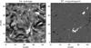 |
Fig. 1 Average Hα line center image (left) and co-spatial Hinode SOT/SP magnetogram (right). The black cross is the reference point for the calculation of the azimuthal profiles (see Sect. 4). |
The SP of SOT performed two raster scans in the Fe i lines at 6301.5 Å and 6302.5 Å. The first one was taken between 9:05 and 9:15 UT, while the second between 9:15−9:25 UT. The SP operated in the Fast Map mode with an effective pixel size of 0″̣32 covering a 50″ × 164″ FOV in 10 min. Inversion of the Stokes spectra was performed by the HAO/CSAC team via the MERLIN code that provided the magnitude of the magnetic field along with its inclination, azimuth, filling factor and several other parameters. MERLIN code uses the Milne-Eddington approximation, according to which the source function varies linearly along the line-of-sight. The magnetic field vector, magnetic fill fraction, line strength, Doppler shift and line broadening are constant along the line-of-sight. The observed line profiles are least-squares fitted using a magnetized component and a scattered light profile. Further information on the inversion procedure can be found at HAO/CSAC team website (http://www.csac.hao.ucar.edu/csac/dataHostSearch.jsp).
3. Data analysis
For the present analysis we used 30 min of continuous Hα observations by the DOT (9:00−9:30 UT on October 15, 2007) and the first raster scan by the SOT/SP. The latter was rotated by 26°̣2 to align with the DOT filtergrams oriented toward the celestial north. We extracted a common FOV, the same quiet solar region studied in Paper I. The morphology of the region is roughly the same as the one described in Paper I, observed half an hour earlier (8:30−9:00 UT). In Fig. 1 we show the co-aligned Hα and SOT/SP data.
We used the Hα intensities at ±0.35 Å and ±0.7 Å to calculate two-dimensional Dopplergrams at each time step using the formula:  (1)which gives the so-called “Doppler signal” (DS). A positive Doppler signal denotes an upward motion of absorbing material. All Doppler signals are relative to a zero reference defined by DS = 0, the mean Doppler signal value of the whole FOV. It should be mentioned that the derived DS values give only a qualitative picture of upward and downward moving material (Tsiropoula 2000).
The three-dimensional magnetic configuration of the chromospheric magnetic field was reconstructed using the current-free (potential) field approximation. In particular, we used the method of Schmidt (1964) that calculates the magnetic field vector above the photosphere using Green’s functions. Unlike the much faster extrapolation involving fast Fourier transforms (e.g. Alissandrakis 1981), Schmidt’s method is analytical and hence much more accurate, resulting to zero current density practically up to machine accuracy. The extrapolation typically requires the normal (vertical) component of the magnetic field vector at the lower boundary (photosphere) that, in our case, is at ~250 km, the formation height of the Fe i lines (Shchukina & Trujillo Buenno 2001). The current-free assumption allows the simplest possible extrapolation and results in a minimum-energy magnetic field vector. It is a reasonable choice for the quiet Sun where there are no conspicuous magnetic polarity inversion lines so the resolved magnetic flux is perhaps left to relax toward a current-free state. An array of recent studies (e.g. Trujillo Bueno et al. 2004; Dominguez Cerdena et al. 2006; Lites et al. 2008; Martinez Gonzalez et al. 2010) emphasize that there is substantial undetected magnetic flux in the quiet Sun. Without detailed knowledge of this flux distribution in our magnetogram, however, this information cannot be included in the extrapolation. On the other hand, small-scale unresolved mixed magnetic polarities, most likely giving rise to small-scale, low-lying flux tubes, should have a minimal macroscopic effect in our extrapolation results. It is also quite unclear whether these features incur any discernible effect in Hα maps, which are the observations correlated with our extrapolation results.
The extrapolation provides the three components, Bx, By and Bz of the magnetic field at equidistant heights, from the photosphere to the corona, with a height step equal to the pixel size of the input photospheric magnetic field (0.32″ or ~235 km, in our case). The line-of-sight (LOS) component of the magnetic field is BLOS = Bz, since the FOV is located at the disk center. We also calculated the transversal (TRANS) component 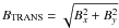 and the inclination θ to the vertical, of the magnetic field vector θ = arctan(BTRANS / BLOS).
In order to produce a view of the plasma topography it is important to consider the distribution of the plasma β with height, which varies from β > 1 in the photosphere to β ≪ 1 in the mid-corona. We assume that the atmospheric stratification of the examined quiet Sun region follows the VAL 3C model (Vernazza et al. 1981). Using the gas pressure Pg at different atmospheric heights given by this model, interpolated at the heights of the extrapolated magnetic field, along with the corresponding field strength we calculated the plasma β, using the equation β = Pg / (B2 / 2μ0). We also calculated, for each pixel of the FOV, the height at which β is of order unity, i.e. the β transition heights, βTH (see e.g. McIntosh et al. 2003).
4. Results
4.1. The photospheric and extrapolated magnetic fields
The region under study (see Fig. 1) is dominated by positive-polarity network bright points (NBPs) which form a large cluster with a center at (x,y) ≈ (25″, 13″) and a smaller one at the upper right part of the FOV with a center at (x,y) ≈ (34″, 32″). In addition to these two stand-out features which have relatively high magnetic fields (B ≃ 1000 G), there are several IN fields of both polarities. When looking at the Hα average intensity image it is easy to see that the two NBP clusters are surrounded by elongated dark mottles that form well-defined rosettes.
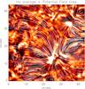 |
Fig. 2 Hα line center intensity image averaged over the duration of the SP raster scan, i.e. between 9:05 and 9:15 UT of October 15, 2007. Overlayed are the field lines of the extrapolated magnetic field. In color in the on-line edition. |
It is commonly assumed that dark mottles map the large-scale magnetic field topology of the chromosphere. A visual comparison between the average Hα image and the extrapolated magnetic field (Fig. 2) justifies this assumption. In this figure the same Hα region of Fig. 1 is shown but it is averaged over the duration of the raster acquisition, that is between 9:05-9:15 UT. Both positive polarity NBP clusters are partly connected to the string of negative polarity fields at the right of the image (see the right panel of Fig. 1 at (x,y) ≈ (40″−43″, 19″−25″), forming structures that resemble closed loops. While many field lines connect the larger NBP cluster to IN magnetic fields, the smaller NBP cluster at the top right of the FOV appears less connected to the IN at the middle of the FOV. Instead, field lines seem to end outside the FOV to the right. This description matches very well with the morphology of the average Hα image. The field lines seem to coincide with positions and orientations of dark mottles and in most cases, mottles are found in areas dense in magnetic field lines. A chain of mottles seen at the lower left corner of the image coincides well with field lines that connect opposite-polarity IN fields. Given the fact that the photospheric magnetic field used as an input for the extrapolation is a raster taken over a period of approximately 10 min and taking into consideration that the assumption of the potential field used for the extrapolation is the simplest approximation that could be used for the chromospheric magnetic field, the correspondence is quite notable.
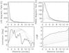 |
Fig. 3 Azimuthal averages of the LOS and transverse field components (first row, left and right panels, respectively), the field inclination in respect to the vertical and the logarithm of plasma β (second row, left and right panels, respectively). In all panels, the solid line corresponds to the base of the extrapolated field, at ~250 km. The dotted lines correspond to extrapolation heights increasing progressively by 235 km from the highest to the lowest curve. In all cases, 0″ corresponds to the center of the rosette (see Fig. 1). |
From now-on we focus our attention to the general behavior of the large rosette which covers the lower part of the FOV. We calculated the azimuthal profiles of the magnetic field parameters at several heights, that is, the LOS and transverse components and the inclination angle of the magnetic field vector, as well as the plasma β, averaging over concentric cycles around a point taken on the NBP cluster (black cross in Fig. 1) considered as the center of the rosette. These profiles are shown in Fig. 3 and give the variation of the corresponding parameters as a function of distance from the center of the rosette. The solid lines show the profiles calculated at the photospheric level, i.e. at ~250 km, while the dotted ones correspond to the rest of the extrapolation heights. In all panels height increases by 235 km from the highest to the lowest curve which corresponds to a height of 2365 km.
The LOS field (upper row, left panel of Fig. 3) peaks at 0″ (core of NBPs) and then reduces fast towards the IN. The transverse field (upper row, right panel) has a peak ~2″ away from the center. This behavior is expected for diverging vertical flux tubes: the transverse component is minimum at the “core” of the NBPs and maximum at their “perimeter”. It then decreases steadily outwards attaining a minimum value at the IN. The strength of both magnetic field components decreases with height, as shown by the dotted lines in the top panels of Fig. 3.
The inclination angle of the magnetic field vector (lower left panel of Fig. 3) is minimum – meaning field mostly normal to the photosphere – near the core of the NBP’s. Moving outward, it increases rapidly, indicating fields with strong tangential (horizontal) components. At the photospheric (~250 km) level the inclination becomes noisy at the IN, as the LOS field amplitude drops very quickly beyond ~4″ from the rosette center to become almost zero. The same is the case for the dotted curves at the extrapolated heights although the distances at which the inclination angle becomes noisy gradually increases. This is because the network flux tubes expand with increasing height to fill increasingly larger volumes at the IN. The distance at which the inclination becomes noisy peaks at ~8″ from the rosette center which is of the order of the extension of dark mottles. Finally, for increasing heights the dotted curves show smaller maxima, i.e., less inclined fields, all the way to the maximum height of 2365 km.
The plasma β (lower row, left panel of Fig. 3) increases steadily with distance towards the IN, where gas pressure dominates. This height variation is expected, since with increasing height β reduces (dotted curves), with the lowest curves being always lower than unity (chromosphere), as gas pressure decreases and magnetic field dominates the plasma dynamics. At the photospheric level (solid line and the first dotted line below it) it is always β > 1 beyond 1″. Very high values of β, especially beyond 6″, are due to the very low values of magnetic field and perhaps the finite (albeit high) spatial resolution smears the local magnetic field strengths, so they should not be considered realistic.
Overall, the extrapolated magnetic field correlates well with the magnetic configuration envisioned from the Hα images and shows a behavior that can be understood physically.
4.2. Power maps and β transition heights
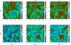 |
Fig. 4 Power maps (each panel in logarithmic scale) at the 3, 5 and 7 min period bands of the DS at 0.35 Å (top row) and 0.70 Å (bottom row) from the Hα line center (power in arbitrary units). Overlayed are the contours of the βTH with the bold contour defining the height of 1.6 Mm. The space between consecutive contours, in βTH, is 0.32 Mm (see text). In color in the on-line edition of the paper. |
We performed a wavelet analysis (Torrence & Compo 1998) on every pixel of the DS time series of images and we constructed 2D power maps in the 3, 5 and 7 min period bands for DS at ±0.35 Å and ±0.70 Å from the Hα line center (see Paper I for details). The power maps are shown in Fig. 4 and have roughly the same appearance with the ones presented in Paper I, where a comparison between the average global wavelet spectra in the rosette and IN regions can also be found. In all panels we have overplotted contours of the βTH (i.e. the heights at which the plasma β becomes equal to 1) which mark the local height of the canopy, a very important critical layer, as far as wave propagation and mode conversion are concerned. These contours start from 0.485 Mm over the network boundaries and increase outwards by 0.235 Mm. The bold contour corresponds to a βTH of 1.6 Mm. A detailed description of the power maps can be found in Paper I. We briefly review these findings below, which also describe the power maps of Fig. 4.
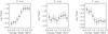 |
Fig. 5 Average of the logarithm of the power of the DS at 0.35 Å from the Hα line center, calculated at the iso-contours of βTH vs. the corresponding canopy height for 3, 5 and 7 min oscillations. |
At photospheric heights, where the Hα ± 0.7 Å wing is formed, the power at 3, 5 and 7 min period bands is enhanced around the network, forming power halos. Higher, in the lower chromosphere, where the Hα ± 0.35 Å is formed, in the 3 and 5 min period bands, these areas are replaced by magnetic shadows, i.e. places of power suppression, more pronounced in the 3 min period band. Interestingly, in the network area the power maps show filamentary structure which, as we have shown in Paper I, correlates very well with the positions of mottles. We have attributed these findings to the interaction between acoustic oscillations and the magnetic fields that mottles outline. In the following we provide more arguments that support this interpretation.
To interpret the observed power distribution one needs to answer the following questions: what is the cause of the enhanced low period power around magnetic flux concentrations, at the photosphere? Why is the low period power reduced around magnetic flux concentrations at the chromosphere? How is it possible to find oscillations with periods of 5 min or larger (which are above the cut-off period), up to chromospheric heights? In the light of high resolution observations such as the ones used in the present study, one has also to determine the effect of the chromospheric fine structure (mottles) on the modulation of the oscillatory power. It is obvious, that the magnetic field and its variation with space (mostly) and time plays a crucial role in the propagation of waves and this is the reason that it is an essential ingredient in all models put forth so far.
Several recent studies have shown that acoustic waves generated at the photosphere and propagating upwards interact with the magnetic field in various ways. In principle, upon meeting the canopy layer, these waves are subject to reflection and refraction, as well as to mode conversion, depending on the attack angle, that is the angle between the propagation direction and the local magnetic field vector (Carlsson & Bogdan 2006). In general the canopy will inhibit the propagation of the high β acoustic waves that propagate vertically. Where the attack angle is low, near the NBP’s acoustic waves go through changing from fast to slow mode waves above the canopy. For larger attack angles refraction, reflection and mode conversion occur and interference patterns between the upward and downward propagating (reflected) waves will increase the power below the canopy. Whether we observe enhanced or suppressed oscillatory power will depend on the relative position of the height-of-formation (HOF) of the bandpass used for the observations and the canopy. If the HOF of the bandpass is located significantly lower than the canopy, then we expect to measure typical IN oscillations, unaffected by the canopy. If, however, the HOF of the bandpass is formed within or above the canopy, then the oscillatory power will be modified.
Additionally, recent observations have detected upward propagating waves with periods higher than 3 min (which is the acoustic cut-off period in the chromosphere). Commonly, it was understood that long period waves should be evanescent at the photosphere, which means that they could not propagate upward, as long as their period is higher than the acoustic cut-off period. It has been shown that in the presence of inclined magnetic fields, near the magnetic concentrations of the network where plasma β is of order unity or lower, p-modes may propagate (leak) to higher atmospheric layers, especially, if the inclination of the magnetic field is significant (Bel & Leroy 1977; Suematsu 1990; De Pontieu et al. 2004). Thus the presence of inclined magnetic field lines near the network boundaries provides a way of channeling otherwise evanescent waves into the chromosphere through what have been called “magneto-acoustic portals” (Jefferies et al. 2006). This mechanism allows the propagation of 5 min and even higher period waves at the chromosphere.
The above stated mechanisms can be used to explain the power maps shown in Fig. 4. In order to show the relationship between the power in the rosette region we have also calculated for every βTH the average logarithm of the DS power contained in the corresponding pixels of the power maps, for each period range. The plots of the logarithm of the DS power versus the βTH (canopy height), along with their 1σ errors are given in Figs. 5 and 6. Furthermore, one should take into account that the Hα ± 0.7 Å wing is formed at the photosphere (~450 km), generally below the β ~ 1 layer, while the Hα ± 0.35 Å wing above it, at the chromosphere, at heights between 900−1500 km (Vernazza et al. 1981; Leenaarts et al. 2006). We will often refer to these bandpasses simply using the words “photosphere” and “chromosphere”, respectively.
At the chromosphere, the 3 min power of the DS is suppressed not only in the area of the large rosette, but over all rosettes observed in the FOV (Fig. 4a). A visual inspection shows that the 1.6 Mm contour (thick line) encloses the areas of suppressed power. Up to this βTH value, the lower the canopy height, the lower the power that is contained in a contour. This can also be seen in Fig. 5a, where one can notice that the power is increasing from the center of the rosette outwards and that beyond 1.6 Mm, the power remains almost constant attaining IN values. This means that the suppression of the 3 min power is of magnetic origin and owes its existence to the relative position between the HOF of the 0.35 Å Hα wing and the canopy which prohibits the 3 min waves to propagate upwards. In the rosette area the power distribution shows a fibrilar structure which, as it has been shown in Paper I, corresponds very well with the distribution of the dark mottles. This suggests that some mottles or parts of them are probably formed below and up to the height of 1.6 Mm and outline the magnetic canopy. A power suppression, but of a smaller extent, is also observed at the 5 min period band over the inner parts of the rosette area, while at its central parts there is a power enhancement (Figs. 4b and 5b). The power enhancement is less obvious in the latter figure than in the former, but it clearly exists as it can also be seen in Fig. 7 described in the following section. On the other hand, a clear power enhancement is observed at the 7 min period band in the area of the rosette. Apart from the refraction of waves propagating upwards at the HOF of 0.35 Å Hα wing, p-mode leakage affects also drastically the distribution of the 5 and 7 min power at the chromosphere, since at the HOF of the Hα ± 0.35 Å wing one samples more inclined flux tubes that are known to constitute mottles. These waves escape the resonant cavity of the solar chromosphere and are guided by the mottles increasing the power at the chromosphere. At larger distances and towards the edges of the rosette, this effect wanes and the suppression of p-modes by the canopy is the dominant feature of the power maps. Point taken, one cannot rule out the possibility that the remarkable enhancement of the 7 min oscillations may be, partly, due to the lifetimes of mottles. As noted in Paper I, these observed enhancement is closely related to mottles and it is possible that the power detected at the chromospheric levels (but also at the photospheric levels) also reflects the temporal dynamics of these structures, hence, defining their lifetime.
At the photosphere, where the Hα ± 0.70 Å DS is formed, the 3, 5 and 7 min power maps show a similar power distribution (Figs. 4d − f), except that the power enhancement is more pronounced in the 7 min period band than in the 5 or the 3 min period bands. This similarity can also be revealed from the corresponding curves of Fig. 4d − f. Power is, on average, enhanced in the central part of the rosette around the NBP cluster and up to canopy heights ≤0.9 Mm. It then decreases with canopy height and remains rather constant for heights larger than 1.2 Mm. This enhancement can be explained if we consider that acoustic waves propagating upwards are reflected on the magnetic canopy. To further support this argument, we note that in Paper I we obtained positive and negative phase differences, at the 5 and 7 min period bands, more positive in the former than in the latter. The negative phase differences point to waves propagating downwards due to their reflection by the inclined mottles. Obviously for canopy heights larger than ~1.2 Mm, much higher than the HOF of the Hα ± 0.7 Å DS, reflection has no detectable effect on the power. Additionally to the reflection of waves, p-mode leakage at the inner parts of the mottles should also be considered to explain the power enhancement observed at the three period bands.
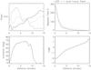 |
Fig. 7 From upper left to lower right: azimuthally averaged power at 3, 5 and 7 min period bands (solid, dotted and dashed lines, respectively) of the DS at the Hα ± 0.35 Å, LOS and transverse field, field inclination angle with respect to the vertical and logarithm of the plasma β. The profiles are averaged over three heights, namely 0.94, 1.17 and 1.4 Mm. |
4.3. Azimuthal profiles of power and magnetic field parameters
We calculated the azimuthal profiles of 3, 5 and 7 min power, as a function of distance from the point considered as the center of the rosette (Fig. 1 but also Paper I). We assume that the Hα wings at 0.7 Å from line center are formed between the formation layer of the Fe i lines and the temperature minimum and therefore we compare the corresponding power with the parameters of the magnetic field at 485 km. For the Hα at 0.35 Å different heights of formation are given in the literature spanning between 900−1500 km (Vernazza et al. 1981; Leenaarts et al. 2006). The corresponding azimuthal profiles of the magnetic field parameters are averaged over the heights of 0.94, 1.17 and 1.4 Mm. The parameters vary smoothly with height (see Sect. 4.1 and Fig. 3) so averaging them over the above mentioned three heights gives us the opportunity to compare the variation of their average value directly with the variation of the DS power at Hα ± 0.35 Å.
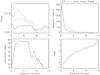 |
Fig. 8 From upper left to lower right: azimuthally averaged power at 3, 5 and 7 min period bands (solid, dotted and dashed lines, respectively), of the DS at Hα ± 0.7 Å, LOS and transverse field, field inclination angle with respect to the vertical and logarithm of the plasma β. The profiles are calculated at 0.485 Mm. |
In the upper left panels of Figs. 7 and 8 we plot the power variation of the DS at Hα ± 0.35 Å and 0.7 Å, respectively, in the 3, 5 and 7 min period bands as a function of the distance from the rosette center. In the upper rows, right panels we show the variation of the LOS and transverse components of the magnetic field. In the bottom rows the magnetic field inclination angle to the vertical is shown (left panels), as well as the logarithm of plasma β (right panels). The variation of these parameters with distance from the NBPs has been described thoroughly in Sect. 4.1. The shape of the power profiles of Figs. 7 and 8 are very similar to the variation of the oscillatory power as a function of the canopy height shown in Figs. 5 and 6. This is reasonable since the canopy height depends on the distance from the NBPs, through its dependence on the magnetic field divergence at the rosette region. A detailed description of the azimuthal profiles of oscillatory power can be found in Paper I, while in the following we attempt to link their most important features with the behavior of the magnetic field.
The oscillatory power of the Hα ± 0.35 Å DS at the 3 min period band has a low peak over the NBPs (up to ~1″). There the inclination angle is lower than 25° (lower left panel of Fig. 7) and waves propagate upwards, following the nearly vertical field lines (Roberts 1983; Khomenko et al. 2008b). Plasma-β is lower than 1 up to ~8″ implying that the Hα ± 0.35 Å DS is formed above or within the canopy in the rosette region. Power is suppressed over the mottles’ area and it is constantly increasing outwards attaining a maximum value over the IN. This power suppression, also called “magnetic shadow”, is very well associated with the β < 1 environment, as can be seen in Fig. 7. A power suppression, although of a smaller extent, is also observed at the power profile of the 5 min period band (dotted line in the first panel of Fig. 7). Between 3″−8″ there is an area of enhanced power described in the previous section and attributed to wave refraction and to p-mode leakage through highly inclined flux tubes. This latter argument is supported by the fact that the maximum of this enhancement is found at ~3″̣>5, where the inclination of the magnetic field is ~60°−70° (second row, left panel of Fig. 7). The power at the 7 min period band shows an enhancement in the inner part of the rosette having a peak at ~3″ (where the inclination angle is of the order of ~60°) and then it decreases constantly outwards. This power enhancement can also be explained as due to wave refraction and p-mode leakage, although, as mentioned above, the possibility to be also partially connected to the mottles’ lifetime cannot be ruled out.
The power variation at the photospheric heights, shown in Fig. 8 differs significantly to the one at the chromosphere, discussed above. The region around the NBPs contains on average substantially more power than the IN in all three period bands due to the almost vertical magnetic fields that allow the waves to propagate upwards. Plasma β is lower than 1 up to a distance of 1″, related to the NBPs and then is always larger than 1 implying that the Hα ± 0.7 Å in the rosette area is formed below the canopy. The power of the oscillations in all three period bands shows an enhancement between 2″ and 10″. The power enhancements correspond to field inclination angles of 65°−75°. The power enhancement in all three period bands can be attributed to the reflection of the upward propagating waves on the canopy. These waves are thus directed downwards and increase the power at the photosphere. The peak at ~2″̣>5 observed at the 5 and 7 min period bands could be due to p-mode leakage, although, since we observe at the photosphere, we sample a smaller portion of the inclined flux tubes and therefore p-mode leakage is expected to have a significantly weaker contribution.
5. Discussion and conclusions
In the present study, high resolution Hα observations of a quiet Sun region obtained by the DOT and corresponding oscillatory power results, presented in Paper I, have been combined with magnetograms obtained by the SOT/SP onboard Hinode in order to improve our understanding of network-IN oscillations and more specifically the interaction between acoustic oscillations and the magnetic field.
Similar past studies have focused on areas which contained extended and/or large concentrations of magnetic elements, such as plages or network near active regions, where the dependence of several observables on the magnetic field strength and/or inclination is easy to examine. However, the advent of high resolution, high precision instruments, such as Hinode’s SOT/SP affords us the opportunity to extend such studies to the quietest regions of the Sun by resolving increasingly finer structures and, hence, dramatically improving our knowledge of the properties of network and IN magnetism (see e.g. Lites et al. 2008).
Small scale magnetic fields of the Sun, present in network clusters, seem to play a leading role in channeling the vast energy budget provided by the convective motions towards the solar atmosphere, either through waves and/or magnetic energy dissipation by reconnection. Hence, knowledge of the three-dimensional magnetic structure, which can be approximated via numerical extrapolations from observed two-dimensional magnetograms, seems to be vital for shedding some light on the link between lower and upper atmospheric layers.
The magnetic field topology of the observed quiet Sun region has been constructed by extrapolation of the photospheric magnetic field using a SOT/SP magnetogram and an analytical potential-field extrapolation method. The extrapolation results show a remarkable correspondence to the observed chromospheric fine structure which is believed to map the magnetic field structure. A similar agreement between potential field extrapolation and X-ray images of a bright point cluster has also been found recently in a multi-wavelength study of a bright point by Perez-Suarez et al. (2008). Of course, it can be argued that nowhere in the Sun can the magnetic field be considered current-free, which is the defining assumption of a potential extrapolation. In fact, even in quiet Sun, Stokes profiles of the magnetic elements show the existence of currents that separate the flux elements from their field-free surroundings (Rezaei et al. 2007). However, it seems that for a time scale of 30 min, one might assume that flux emergence and electric currents do not alter the average global structure of the chromospheric magnetic field. Especially when one wants to compare an average magnetic configuration, where no dissipative processes are involved, with the distribution of oscillatory power on the FOV (like e.g. in McIntosh et al. 2003; Muglach et al. 2005 and the present study), the potential field approximation is the most suitable choice.
Unfortunately, the obtained magnetic field structure cannot be used for the detection of reconnection events, if present. Apart from the lack of spatial and temporal resolution observations which would allow the tracking of locations where reconnection might occur, the potential field by definition does not involve such processes. Nonetheless, valuable information can be extracted for the behavior of waves by comparison of the field extrapolation results with oscillations in different frequencies. We have concentrated on the behavior of the 3, 5 and 7 min oscillations which are characteristic frequencies of IN and network oscillations in the literature.
It has been shown that the relative positions of the magnetic canopy, the inclination of the magnetic field and the HOF of the particular wavelength of the line used for the observations, define the modulation of the oscillatory power (Rosenthal et al. 2002; Bogdan et al. 2003). When waves, that propagate upwards from the photosphere into the chromosphere, reach the canopy they undergo mode conversion, refraction and reflection. The crucial parameter for what happens to the waves is the angle between the magnetic field and the k-vector: the attack angle. At small attack angles the waves go through as acoustic waves changing from being fast mode waves in the high-β regime to being slow mode waves in the low-β regime. At angles larger than 30° there is both transmission of fast mode waves as slow mode propagating along the field lines and reflection. At even larger angles ≈50° most of the waves are refracted or reflected and return as a fast mode creating an interference pattern between the upward and downward propagating waves. In this work we were able to obtain the magnetic field inclination and the plasma-β in a rosette region and thus to locate the canopy. Our results show that Hα ± 0.35 Å is formed above or within the canopy, while Hα ± 0.7 Å is formed below the canopy. This finding can explain the power deficits and power enhancements observed at the DS of the rosette region. Thus we found a power suppression (magnetic shadow) in the 3 and 5 min period bands at the Hα ± 0.35 Å DS which is formed above the canopy. On the other hand, at the Hα ± 0.7 Å DS which is formed below the canopy the reflection of acoustic waves on the β = 1 surface increases the power forming a power halo. We indirectly inferred that some mottles or parts of them probably form at relatively low heights, lower than 1.6 Mm, and provide the locations where mode conversion, reflection and refraction of waves are more likely to occur. It has also been suggested that long period waves (e.g. 5 or 7 min), which are considered to be evanescent, can escape the acoustic cavity of the chromosphere due to p-mode leakage.
More specifically, our study has shown that the 3 min power suppression at the Hα ± 0.35 Å in the rosette region is indeed due to the magnetic canopy which inhibits the propagation of these low period waves. This is confirmed by the remarkable correspondence between the magnetic shadow and the βTH contours that map the canopy and further supports our finding in Paper I that 3 min waves do not propagate vertically through this critical surface.
This power suppression is also somehow evident in the 5 min period band in the inner part of the rosette. In addition to that, it is interesting to note that our results indicate a peak of the 5 min power at a distance where the inclination angle of the magnetic field is ~60°−70°, which appears to agree with existing works concerning the leakage of high-period p-modes in highly inclined tubes. It is worth mentioning at this point that it is well-established in the literature that their oscillatory behavior of mottles is altogether different to the IN and that 5 min oscillations are common in mottle studies (see e.g. Tsiropoula et al. 2009, and references therein).
The aforementioned findings concerning the power distribution and its relation to the magnetic canopy are in close agreement with those of McIntosh et al. (2003), who found that the areas of suppressed power over and around the network fall strikingly well within the contours of βTH. Their TRACE observations also show that the lower the transition height, the lower the power. On the other hand, as they reported, MDI photospheric velocity power does not show any correlation with these contours, except for the innermost parts of the network, where indeed one can see again a suppression of oscillatory power. In the present study, however, we found that the increased power is also linked to the canopy, even though the increased power is not distributed smoothly inside the contours. This is due to the presence of mottles (not sampled by MDI dopplergrams) which seem to provide the loci where wave reflection and refraction occur. Our high resolution Hα data exhibit the same aspects of the interaction between acoustic oscillations and the magnetic field, even though the morphology of the chromosphere in Hα and TRACE continua differ significantly.
Concerning the 7 min oscillations, our comparison of the magnetic field configuration with the corresponding oscillation power distribution indicates that the observed power enhancement is mostly due to reflection and refraction of waves. At chromospheric layers the observed power enhancement is mostly due to waves that refract at the canopy surface, but also to p-mode leakage due to the large inclinations of the magnetic field. At lower layers close to the photosphere this enhancement is mostly due to wave reflection at the overlying canopy. However, as already mentioned, part of the 7 min oscillatory power could also be attributed to the lifetime of mottles thus explaining the increased 7 min power in the rosette area and its distribution in a fibrilar pattern.
As a final note, we should point out that the wide range of heights that contribute to the formation of the Hα make this line, albeit complicated, a valuable tool for understanding the interconnection between photospheric and chromospheric plasma dynamics. In forthcoming works we plan to incorporate more observations (TRACE, MDI, G-band and Ca ii h filtergrams) to investigate the interconnection between different layers of the solar atmosphere and gain a better understanding of the connection between the chromospheric fine structure and wave properties and propagation.
Acknowledgments
The DOT is operated by Utrecht University at the Spanish Observatorio del Roque de los Muchachos of the Instituto de Astrofísica de Canarias. The authors thank P. Sütterlin for the DOT observations and R. Rutten for the data reduction. These observations have been funded by the Optical Infrared Coordination network (OPTICON, http://www.ing.iac.es/opticon), a major international collaboration supported by the Research Infrastructures Programme of the European Commission’s sixth Framework Programm. Hinode is a Japanese mission developed and launched by ISAS/JAXA, collaborating with NAOJ as a domestic partner, NASA and STFC (UK) as international partners. Scientific operation of the Hinode mission is conducted by the Hinode science team organized at ISAS/JAXA. This team mainly consists of scientists from institutes in the partner countries. Support for the post-launch operation is provided by JAXA and NAOJ (Japan), STFC (UK), NASA, ESA, and NSC (Norway). Hinode SOT/SP Inversions were conducted at NCAR under the framework of the Community Spectro-polarimtetric Analysis Center (CSAC; http://www.csac.hao.ucar.edu). The authors also thank the International Space Science Institute (ISSI) in Bern, Switzerland, for the hospitality provided to the members of the team on “Solar small-scale transient phenomena and their role in coronal heating” as well as the members of the team for fruitful discussions.
References
- Alissandrakis, C. E. 1981, A&A, 100, 197 [NASA ADS] [Google Scholar]
- Bel, N., & Leroy, B. 1977, A&A, 55, 239 [NASA ADS] [Google Scholar]
- Bogdan, T. J., Carlsson, M., Hansteen, V., et al. 2003, ApJ, 599, 626 [NASA ADS] [CrossRef] [Google Scholar]
- Braun, D. C., Duvall, T. L., Jr.,Labonte, B. J., et al. 1992, ApJ, 391, L113 [NASA ADS] [CrossRef] [Google Scholar]
- Brown, T. M., Bogdan, T. J., Lites, B. W., & Thomas, J. H. 1992, ApJ, 394, L65 [NASA ADS] [CrossRef] [Google Scholar]
- Carlsson, M., & Bogdan, T. J. 2006, Philos. Trans. R. Soc. London A, 364, 395 [NASA ADS] [CrossRef] [Google Scholar]
- Cauzzi, G., Falchi, A., & Falciani, R. 2000, A&A, 357, 1093 [NASA ADS] [Google Scholar]
- De Pontieu, B., Erdélyi, R., & James, S. P. 2004, Nature, 430, 536 [NASA ADS] [CrossRef] [PubMed] [Google Scholar]
- Deubner, F. L., & Fleck, B. 1989, A&A, 213, 423 [NASA ADS] [Google Scholar]
- Deubner, F. L., & Fleck, B. 1990, A&A, 228, 506 [NASA ADS] [Google Scholar]
- Dominguez Cerdena, I., Sanchez Almeida, J., & Kneer, F. 2006, ApJ, 636, 496 [NASA ADS] [CrossRef] [Google Scholar]
- Finsterle, W., Jefferies, S. M., Cacciani, A., et al. 2004, ApJ, 613, L185 [Google Scholar]
- Hanasoge, S. M. 2009, A&A, 503, 595 [NASA ADS] [CrossRef] [EDP Sciences] [Google Scholar]
- Hindman, B. W., & Brown, T. M. 1998, ApJ, 504, 1029 [NASA ADS] [CrossRef] [Google Scholar]
- Jacoutot, L., Kosovichev, A., Wray, A., & Mansour, N. 2009, ASPC, 416 [Google Scholar]
- Jain, R., & Haber, D. 2002, A&A, 387, 1092 [NASA ADS] [CrossRef] [EDP Sciences] [Google Scholar]
- Jefferies, S. M., McIntosh, S. W., Armstrong, J. D., et al. 2006, ApJ, 648, L151 [Google Scholar]
- Judge, P. G., Tarbell, T. D., & Wilhelm, K. 2001, ApJ, 554, 424 [NASA ADS] [CrossRef] [Google Scholar]
- Khomenko, E., & Collados, R. 2009, A&A, 506, L5 [NASA ADS] [CrossRef] [EDP Sciences] [Google Scholar]
- Khomenko, E., Collados, M., & Felipe, T. 2008a, Solar Phys., 251, 589 [Google Scholar]
- Khomenko, E., Centeno, R., Collados, M., & Trujillo Bueno, J. 2008b, ApJ, 676, L85 [NASA ADS] [CrossRef] [Google Scholar]
- Kontogiannis, I., Tsiropoula, G., & Tziotziou, K. 2010, A&A, 510, A41 (Paper I) [NASA ADS] [CrossRef] [EDP Sciences] [Google Scholar]
- Kosugi, T., Matsuzaki, K., Sakao, T., et al. 2007, Solar Phys., 243, 3 [Google Scholar]
- Krijger, J. M., Rutten, R. J., Lites, B. W., et al. 2001, A&A, 379, 1052 [NASA ADS] [CrossRef] [EDP Sciences] [Google Scholar]
- Kuridze, D., Zaqarashvili, T. V., Shergelashvili1, B. M., & Poedts, S. 2008, Ann. Geophys., 26, 2983 [Google Scholar]
- Kuridze, D., Zaqarashvili, T. V., Shergelashvili, B. M., & Poedts, S. 2009, A&A, 505, 763 [NASA ADS] [CrossRef] [EDP Sciences] [Google Scholar]
- Leenaarts, J., Rutten, R. J., Sütterlin, P., Carlsson, M., & Uitenbroek, H. 2006, A&A, 449, 1209 [NASA ADS] [CrossRef] [EDP Sciences] [Google Scholar]
- Lites, B. W., Rutten, R. J., & Kalkofen, W. 1993, ApJ, 414, 345L [NASA ADS] [CrossRef] [Google Scholar]
- Lites, B. W., Kubo, M., Socas-Navarro, H., et al. 2008, ApJ, 672, 1237 [NASA ADS] [CrossRef] [Google Scholar]
- Martinez Gonzalez, M. J., Manso Sainz, R., Asensio Ramos, A., Lopez Ariste, A., & Bianda, M. 2010, ApJ, 711, L57 [NASA ADS] [CrossRef] [Google Scholar]
- McIntosh, S. W., & Judge, P. G. 2001, ApJ, 561, 420 [NASA ADS] [CrossRef] [Google Scholar]
- McIntosh, S. W., Fleck, B., & Judge, P. G. 2003, A&A, 405, 769 [NASA ADS] [CrossRef] [EDP Sciences] [Google Scholar]
- Muglach, K. 2003, A&A, 401, 685 [Google Scholar]
- Muglach, K., Hofmann, A., & Staude, J. 2005, A&A, 437, 1055 [NASA ADS] [CrossRef] [EDP Sciences] [Google Scholar]
- Muller, R., Dollfus, A., Montagne, M., Moity, J., & Vigneau, J. 2000, A&A, 359, 373 [NASA ADS] [Google Scholar]
- Pérez-Suárez, D., Maclean, R. C., Doyle, J. G., et al. 2008, A&A, 492, 575 [NASA ADS] [CrossRef] [EDP Sciences] [Google Scholar]
- Reardon, K. P., Uitenbroek, H., & Cauzzi, G. 2009, A&A, 500, 1239 [NASA ADS] [CrossRef] [EDP Sciences] [Google Scholar]
- Rezaei, R., Steiner, O., Webemeyer-Böhm, S., et al. 2007, A&A, 476, L33 [NASA ADS] [CrossRef] [EDP Sciences] [Google Scholar]
- Roberts, B. 1983, Solar Phys., 87, 77 [NASA ADS] [CrossRef] [Google Scholar]
- Rosenthal, C. S., Bogdan, T. J., Carlsson, M., et al. 2002, ApJ, 564, 508 [NASA ADS] [CrossRef] [Google Scholar]
- Rutten, R. J., Hammerschlag, R. H., Bettonvil, F. C. M., et al. 2004, A&A, 413, 1183 [NASA ADS] [CrossRef] [EDP Sciences] [Google Scholar]
- Schmidt, H. U. 1964, in AAS-NASA Symposium on the Physics of Solar Flares, ed. W. N. Hess, Washington D.C., NASA SP-50, 107 [Google Scholar]
- Schunker, H., & Braun, D. C. 2010, Solar Physics, in press [arXiv:0911.3042] [Google Scholar]
- Shchukina, N., & Trujillo-Bueno, J. 2001, ApJ, 550, 970 [NASA ADS] [CrossRef] [Google Scholar]
- Suematsu, Y. 1990, Lect. Notes Phys., 367, 211 [Google Scholar]
- Suematsu, Y., Wang, H., & Zirin, H. 1995, ApJ, 450, 411 [NASA ADS] [CrossRef] [Google Scholar]
- Thomas, J. H., & Stanchfield, D. C. H. 2000, ApJ, 537, 1086 [NASA ADS] [CrossRef] [Google Scholar]
- Torrence, C., & Compo, G. P. 1998, Bull. Amer. Meteor. Soc., 79, 61 [CrossRef] [Google Scholar]
- Trujillo Bueno, J., Shchukina, N., & Asensio Ramos, A. 2004, Nature, 430, 326 [Google Scholar]
- Tsiropoula, G. 2000, New Astr., 5, 1 [Google Scholar]
- Tsiropoula, G., Tziotziou, K., Schwartz, P., & Heinzel, P. 2009, A&A, 493, 217 [NASA ADS] [CrossRef] [EDP Sciences] [Google Scholar]
- Tsuneta, S., Suematsu, Y., Ichimoto, K., et al. 2008, Solar Phys., 249, 197 [Google Scholar]
- Tziotziou, K., Tsiropoula, G., & Mein, P. 2004, A&A, 423, 1133 [NASA ADS] [CrossRef] [EDP Sciences] [Google Scholar]
- Vecchio, A., Cauzzi, G., Reardon, K. P., et al. 2007, A&A, 461, L1 [NASA ADS] [CrossRef] [EDP Sciences] [Google Scholar]
- Vernazza, J. E., Avrett, E. H., & Loeser, R. 1981, ApJS, 45, 635 [NASA ADS] [CrossRef] [Google Scholar]
- von Uexküll, M., Kneer, F., Malherbe, J. M., & Mein, P. 1989, A&A, 208, 290 [NASA ADS] [Google Scholar]
- Wang, H., Tang, F., Zirin, H., & Wang, J. 1996, Solar Phys., 165, 223 [Google Scholar]
All Figures
|
Fig. 1 Average Hα line center image (left) and co-spatial Hinode SOT/SP magnetogram (right). The black cross is the reference point for the calculation of the azimuthal profiles (see Sect. 4). |
| In the text | |
|
Fig. 2 Hα line center intensity image averaged over the duration of the SP raster scan, i.e. between 9:05 and 9:15 UT of October 15, 2007. Overlayed are the field lines of the extrapolated magnetic field. In color in the on-line edition. |
| In the text | |
|
Fig. 3 Azimuthal averages of the LOS and transverse field components (first row, left and right panels, respectively), the field inclination in respect to the vertical and the logarithm of plasma β (second row, left and right panels, respectively). In all panels, the solid line corresponds to the base of the extrapolated field, at ~250 km. The dotted lines correspond to extrapolation heights increasing progressively by 235 km from the highest to the lowest curve. In all cases, 0″ corresponds to the center of the rosette (see Fig. 1). |
| In the text | |
|
Fig. 4 Power maps (each panel in logarithmic scale) at the 3, 5 and 7 min period bands of the DS at 0.35 Å (top row) and 0.70 Å (bottom row) from the Hα line center (power in arbitrary units). Overlayed are the contours of the βTH with the bold contour defining the height of 1.6 Mm. The space between consecutive contours, in βTH, is 0.32 Mm (see text). In color in the on-line edition of the paper. |
| In the text | |
|
Fig. 5 Average of the logarithm of the power of the DS at 0.35 Å from the Hα line center, calculated at the iso-contours of βTH vs. the corresponding canopy height for 3, 5 and 7 min oscillations. |
| In the text | |
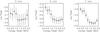 |
Fig. 6 Same as Fig. 5, but for DS at 0.70 Å from the Hα line center. |
| In the text | |
|
Fig. 7 From upper left to lower right: azimuthally averaged power at 3, 5 and 7 min period bands (solid, dotted and dashed lines, respectively) of the DS at the Hα ± 0.35 Å, LOS and transverse field, field inclination angle with respect to the vertical and logarithm of the plasma β. The profiles are averaged over three heights, namely 0.94, 1.17 and 1.4 Mm. |
| In the text | |
|
Fig. 8 From upper left to lower right: azimuthally averaged power at 3, 5 and 7 min period bands (solid, dotted and dashed lines, respectively), of the DS at Hα ± 0.7 Å, LOS and transverse field, field inclination angle with respect to the vertical and logarithm of the plasma β. The profiles are calculated at 0.485 Mm. |
| In the text | |
Current usage metrics show cumulative count of Article Views (full-text article views including HTML views, PDF and ePub downloads, according to the available data) and Abstracts Views on Vision4Press platform.
Data correspond to usage on the plateform after 2015. The current usage metrics is available 48-96 hours after online publication and is updated daily on week days.
Initial download of the metrics may take a while.