| Issue |
A&A
Volume 523, November-December 2010
|
|
|---|---|---|
| Article Number | A81 | |
| Number of page(s) | 11 | |
| Section | Cosmology (including clusters of galaxies) | |
| DOI | https://doi.org/10.1051/0004-6361/201015198 | |
| Published online | 18 November 2010 | |
Cold fronts and multi-temperature structures in the core of Abell 2052
1
SRON Netherlands Institute for Space Research,
Sorbonnelaan 2,
3584 CA
Utrecht,
The Netherlands
e-mail: This email address is being protected from spambots. You need JavaScript enabled to view it.
2
Kavli Institute for Particle Astrophysics and Cosmology, Stanford
University, 382 via Pueblo
Mall, Stanford,
CA
94305-4060,
USA
3
Astronomical Institute, Utrecht University,
PO Box 80000,
3508 TA
Utrecht, The
Netherlands
Received: 11 June 2010
Accepted: 13 August 2010
Abstract
Context. The physics of the coolest phases in the hot intra-cluster medium (ICM) of clusters of galaxies is yet to be fully unveiled. X-ray cavities blown by the central active galactic nucleus (AGN) contain enough energy to heat the surrounding gas and stop cooling, but locally blobs or filaments of gas appear to be able to cool to low temperatures of 104 K. In X-rays, however, gas with temperatures lower than 0.5 keV is not observed.
Aims. We aim to find spatial and multi-temperature structures in the hot gas of the cooling-core cluster Abell 2052 that contain clues on the physics involved in the heating and cooling of the plasma.
Methods. 2D maps of the temperature, entropy, and iron abundance are derived from XMM-Newton data of Abell 2052. For the spectral fitting, we use differential emission measure (DEM) models to account for the multi-temperature structure.
Results. About 130 kpc South-West of the central galaxy, we discover a discontinuity in the surface brightness of the hot gas which is consistent with a cold front. Interestingly, the iron abundance jumps from ~0.75 to ~0.5 across the front. In a smaller region to the North-West of the central galaxy we find a relatively high contribution of cool 0.5 keV gas, but no X-ray emitting gas is detected below that temperature. However, the region appears to be associated with much cooler Hα filaments in the optical waveband.
Conclusions. The elliptical shape of the cold front in the SW of the cluster suggests that the front is caused by sloshing of the hot gas in the clusters gravitational potential. This effect is probably an important mechanism to transport metals from the core region to the outer parts of the cluster. The smooth temperature profile across the sharp jump in the metalicity indicates the presence of heat conduction and the lack of mixing across the discontinuity. The cool blob of gas NW of the central galaxy was probably pushed away from the core and squeezed by the adjacent bubble, where it can cool efficiently and relatively undisturbed by the AGN. Shock induced mixing between the two phases may cause the 0.5 keV gas to cool non-radiatively and explain our non-detection of gas below 0.5 keV.
Key words: galaxies: clusters: general / galaxies: clusters: intracluster medium / galaxies: clusters: individual: Abell 2052 / X-rays: galaxies: clusters
© ESO, 2010
1. Introduction
Our understanding of heating and cooling mechanisms operating in the hot intra-cluster medium (ICM) in the cores of clusters of galaxies is not yet complete. The cooling times of the relatively dense X-ray emitting plasma in the central region are short compared to the Hubble time, which lead to the theory of cooling-flows (e.g. Fabian 1994). The first cluster observations with the high-resolution Reflection Grating Spectrometer (RGS, den Herder et al. 2001) aboard XMM-Newton show, however, that the amount of cool gas in the centre of clusters is much smaller than expected (Peterson et al. 2001; Tamura et al. 2001; Kaastra et al. 2001; Peterson et al. 2003). In recent years, it has been suggested that this lack of cool gas can be explained by feedback from the central active galactic nucleus (AGN). The relativistic plasma in the jets originating from this accreting central super-massive black hole creates cavities in the hot X-ray emitting gas, which appear as dark regions in X-ray images of clusters. The energy enclosed in these plasma bubbles appears to be enough to balance the cooling flow (e.g. Churazov et al. 2002; Brüggen & Kaiser 2002; Bîrzan et al. 2004). The mechanism responsible for gently transferring the energy from the bubbles to the X-ray gas is, however, still unclear.
The lowest temperatures detected in clusters through X-rays are about 0.5 keV, which appears to be a universal low-temperature floor for clusters and groups. However, these low-temperature regions are usually found in clusters which show AGN activity, like, for example, Hydra A (McNamara et al. 2000), Perseus (Sanders & Fabian 2007), and M 87 (e.g. Werner et al. 2010). This appears contradictory, because AGN are supposed to heat the gas. Studies of the volume filling fraction of this 0.5 keV component (e.g. Sanders & Fabian 2002; Sanders et al. 2004) show that the cool gas is actually distributed in clumps or filaments. This suggests that gas can cool locally to low temperatures despite the fact that it is embedded in hotter gas. In many clusters these cool regions are seen at the same position as bright Hα regions and filaments detected in optical images of these clusters. The connection between the 0.5 keV gas and Hα emission is an important piece of the puzzle of understanding heating and cooling in cluster cores.
On slightly larger scales, disturbances due to merger events cause the dark matter and subsequently the hot X-ray gas to oscillate in the deep gravitational potential well of a cluster. This sloshing of gas is usually recognised in X-ray images through asymmetries and jumps in the surface brightness of the hot gas. The underlying density discontinuity, also called a cold front, marks the boundary between relatively cool moving gas from the central part of the cluster and the hot gas in the outer regions (see Markevitch & Vikhlinin 2007, for a review). The slow release of mechanical energy from the sloshing movements and the mixing of hot gas from the outer parts into the cooling core may both contribute to heat the inner parts of the cluster in concurrence with the AGN. Sloshing is probably also an important mechanism for transporting metals from the metal-rich core to the metal-poor outer parts (Simionescu et al. 2010).
The cluster of galaxies Abell 2052 is also a bright cool-core cluster in X-rays showing AGN activity and Hα regions (Blanton et al. 2001). The cluster was detected and studied in the 1970’s (Giacconi et al. 1972; Heinz et al. 1974). Abell 2052 is also extensively studied with the current generation of X-ray observatories. It was member of several samples of clusters observed with ASCA (Finoguenov et al. 2001) and XMM-Newton (e.g. Kaastra et al. 2004a; Tamura et al. 2004; de Plaa et al. 2007). Chandra images (Blanton et al. 2001, 2003, 2009) show evidence of AGN feedback by the central radio source 3C 317 (Zhao et al. 1993). In the inner core (<1.0′) of the cluster, the X-ray image shows bubbles which are associated with the radio lobes of 3C 317. The energy contained in the cavities is thought to effectively heat the intra-cluster medium (ICM). In addition, density discontinuities, probably shocks have been detected by Chandra (Blanton et al. 2009) just outside the region with the bubbles.
We have obtained a long observation of Abell 2052 with XMM-Newton, which was performed in 2007. In this paper, we combine this new observation with an older AO1 observation of ~40 ks and study the thermodynamics in and around the core. We use the spatially resolved spectra from the European Photon Imaging Camera (EPIC) to make two-dimensional maps.
In our analysis, we use H0 = 70 km s-1 Mpc-1, Ωm = 0.3, and ΩΛ = 0.7. At the redshift of Abell 2052 (z = 0.0348), an angular distance of 1′ corresponds to 42 kpc. The elemental abundances presented in this paper are given relative to the proto-solar abundances from Lodders (2003). Measurement errors are given at 68% confidence level.
2. Data analysis
Abell 2052 has been observed with XMM-Newton in two observation campaigns. Two observations have been performed in 2000 with a total exposure time of 37 ks and another ten exposures were obtained in 2007 with a total observing time of 221 ks.
The event files for the MOS and pn detectors are re-produced using the standard SAS 9.0.0 pipeline tools. In order to reduce the soft-proton background, we filter the data with a 10–12 keV count-rate threshold. We determine the threshold for the 2000 (AO1) and 2007 (AO4) data separately. For the AO4 data we combined all the separate observations to obtain one 10–12 keV light curve per instrument. A count-rate histogram created from this light curve with 100 s wide bins is fitted with a Gaussian to determine the count rate of the quiescent emission (N). We then define the minimum and maximum count rate (T) to be  , which is the 3σ deviation from the Poissonian mean. We apply this to both the AO1 and AO4 data sets. For the AO1 data, we obtain allowed count rates in the range 0.01–0.18 (MOS1), 0.01–0.18 (MOS2), and 0.11–0.43 (pn) in units counts s-1. The average rate in counts s-1 in the AO4 data was somewhat higher: 0.03–0.27 (MOS1), 0.04–0.28 (MOS2), and 0.28–0.70 (pn). This is due to the secular evolution of the XMM-Newton instrumental background.
In Table 1, we list all used observations of Abell 2052 with their respective exposure times after filtering for flares. Two other observations are discarded, because the count rate was above the threshold during the entire exposure. Only eight of the brightest point sources in the field were selected by eye using a combined image of MOS and pn. Regions with a radius of 15′′ around these sources were subsequently excluded from the data set.
List of observation IDs used for the analysis with their useful exposure time in ks after flare filtering.
2.1. Creating maps
In order to resolve structures in temperature and iron abundance, we divide the data in small regions from which spectra can be extracted. To obtain sufficient signal-to-noise per spatial bin, we use the Weighted Voronoi Tessellation (WVT) binning algorithm by Diehl & Statler (2006), which is a generalization of the Cappellari & Copin (2003) Voronoi binning algorithm. We apply the binning to the total background subtracted image and create maps with a signal-to-noise of 150σ per bin. Because of the relatively low surface brightness of the source compared to the X-ray background in the outer parts of the cluster, we only select bins within a radius of 4′ (~168 kpc) around the centre of the central cD galaxy.
For every bin, we extract the event files and spectra. Then, we calculate the response matrices and effective area files for all spatial bins using one AO1 pointing and one AO4 pointing. These response and effective area files are also used for the other pointings of the same AO in order to reduce computing time. We checked that the response is stable enough within one AO. Also, the pointings within one AO were very similar, causing the extraction regions defined in WCS coordinates to cover the same area in detector coordinates for every pointing. Therefore, using one response matrix per spatial bin per AO is justified. As we are mainly interested in relative differences between bins, we adopt a relatively simple background treatment for the maps. We subtract a scaled filter wheel closed spectrum from the source spectrum. The scaling factor is based on the out-of-field-of-view events in MOS. The spectra for each bin are fitted simultaneously using the SPEX spectral fitting package. The cosmic X-ray background (CXB) is included as a set of model components in the fit. For the NH we use the Galactic value of 2.71 × 1020 cm-2 (Kalberla et al. 2005).
2.2. Fitting interesting regions
Apart from spectra extracted from binned maps, we also carefully analyse spectra extracted from certain interesting regions that we identify in the maps. In addition, the parameters of the CXB components need to be estimated, because they are needed for fitting the maps. Therefore, we use a separate procedure for these high signal-to-noise spectra. The background treatment is very important when fitting spectra extracted from the outer regions of a cluster, where the flux of the cluster emission is comparable to the background.
Correcting for all the various background components in XMM-Newton data is very challenging, because many components either depend on the position on the sky or depend on the epoch of observation. The fact that we have obtained a lot of relatively short exposures with different background conditions, demands a careful treatment of all the components. Although there are very well constructed methods like, for example, Snowden et al. (2008), there are a number of drawbacks when they are applied to this data set. The success of these methods strongly depends on the events registered outside the XMM-Newton field of view. Because the pn instrument has very small out-of-field-of-view regions, their method is practically unusable for pn data. Secondly, the amount of counts in the out-of-field of view regions is rather small for short exposure times, which puts a relatively large uncertainty on the derived scaling factor for the instrumental background. This drawback can be avoided by stacking event files, but only if the gain and background were similar during the observations. Here, we present a method in which we model all the background components during spectral fitting without subtracting any background spectrum beforehand. This allows us to use both EPIC MOS and pn data.
The first set of background components that we model is the instrumental background due to hard particles. These are mostly very energetic particles that enter the detector from all directions. The total spectrum of these components can be observed when the “closed” filter has been chosen. The typical spectrum is composed of a broken power law and several instrumental fluorescence lines. Since these background events are not caused by reflected X-rays from the mirror, the models should not be folded with the effective area (ARF). The normalisation of the broken power law can vary in time independently of the lines. During the mission, the normalisation of the power-law component has slowly increased. We assume that the power-law index does not change significantly with time. To find the average parameters of the power law, we fit the spectra derived from the merged closed filter observations provided by the XMM-Newton science operations centre (SOC). For every source region that we analyse, we extract a spectrum from a closed-filter region with the same detector coordinates. Then, we fit a broken power-law model to the data including delta lines to model the fluorescence lines (see Table 2 for a list of lines for MOS and pn). The parameters for the power-law index, the change in index, and the break energy are used when fitting the source spectrum. In the fit, the normalisations of the broken power law and the delta lines are allowed to vary within a bandwidth of a factor of two with respect to the best fit closed-filter results. This is to limit the possible effect that genuine spectral features are compensated in the fit by increasing the normalisation of background components.
The second set of background components is the cosmic X-ray background (CXB). The high-energy part of this background spectrum is dominated by unresolved point sources, which is described well by a power-law component with a slope of Γ = 1.41 (De Luca & Molendi 2004). We fix the normalisation of the power law to their value which corresponds to a 2–10 keV flux of 2.24 × 10⁻¹⁴ W m-2 deg-2. In this paper, we do not correct for the exclusion of point sources which affects the flux of this component, because we mainly focus on the inner 5′ of the cluster where the influence of small variations in this component are negligible. Below 2 keV, the spectrum consists of contributions from the local-hot bubble and Galactic thermal emissions (e.g. Kuntz & Snowden 2000, 2008). We model these components with two single-temperature plasma models assuming Collisional Ionisation Equilibrium (CIE). The coolest component is associated with the Local Hot Bubble and is not affected by absorption. The temperatures of the two components can vary slightly over the sky. Therefore, we fit the temperature and normalisations of these components in a 9.0′–12′ annulus around the cluster centre in the 0.4–12 keV band. In this annulus, the normalisations and temperatures are well constrained. We set the temperatures for the two components to their (rounded) best fit values of 0.120 (± 0.004) keV and 0.290 (± 0.006) keV, respectively. The 0.1–2.5 keV flux of the 0.12 keV component is (5.03 ± 0.15) × 10-14 W m-2 deg-2 and for the 0.29 keV component it is (1.87 ± 0.04) × 10-14 W m-2 deg-2. We assume solar abundances for the Local Hot Bubble and use 0.7 times solar for the more distant 0.29 keV component, which was a typical value determined from the fits. With this set of models we have a good parametrisation of the CXB which can be applied to spectra extracted from other areas within the field of view.
Modeled instrumental lines for EPIC MOS and pn.
There are two other potentially important background components: charge exchange emission from interactions between the solar wind and solar-system material, and quiescent soft-protons. The charge exchange emission consists of time variable line emission below 1 keV. We checked the low-energy light curves for variability, but no significant flares were found. Soft-proton flares were already removed from the data by rather strict filtering. A low quiescent level of soft-proton contamination is probably still present. To get an estimate of the soft-proton flux, we compared the out-of-field-of-view areas with the count rate in the field of view in the 10–12 keV band. We did not find a significant difference between the two count rates, which implies that this component is indeed very weak. Another check would be whether the derived spectral models are stable with respect to the observation epoch and soft-proton rate. We have fitted the AO1 and AO4 spectra extracted from a region in the centre of the cluster separately and find that the derived models parameters, like temperature and iron abundance, are consistent within the error bars and within 5%. Therefore, we ignore the soft-proton contribution for now and let it be partly compensated by the normalisation of the power law of the instrumental background. An independent measurement of the soft-proton flux would be necessary to include this component in the model.
2.3. Surface brightness profiles
For diagnostics of density discontinuities it is useful to create profiles of, for example, surface brightness. We derive these profiles using images extracted from the event files, background images, and exposure maps. Regions are selected using a mask image. The images are extracted with the same WCS reference coordinates, which means that the pixels in every image represent the same area on the sky. We add the source counts, background counts, and exposure values for every pixel in all pointings and then we calculate the background subtracted count rate. We bin the profile in 0.1′ bins and calculate the angular distance scale with respect to the central cD galaxy. Throughout this paper, we use the coordinates α15h16m44.47sδ 7°01′18.47′′ for the centre of the cluster.
3. Spectral models
For spectral fitting we use the publicly available SPEX spectral fitting package (Kaastra et al. 1996). The code contains several methods to fit multi-temperature differential emission measure (DEM) models to X-ray spectra. For cluster emission, the Gaussian (gdem) and power-law (wdem) parametrisation have been successfully fitted before. However, from the fits it is usually not possible to distinguish between these different DEM shapes (e.g. de Plaa et al. 2006).
3.1. GDEM
The first DEM model that we use is a Gaussian differential emission measure (GDEM) distribution. The Gaussian is either defined on a logarithmic temperature grid (log T) or a linear grid:  (1)For the logarithmic grid, x = log T and x0 = log T0 where T0 is the central temperature of the distribution. In the linear case, x = T and x0 = T0. The width of the Gaussian is σT.
3.2. WDEM
The second empirical model that we use in this paper is known as wdem (Kaastra et al. 2004a; de Plaa et al. 2005), which proved to be successful in fitting cluster cores (e.g. Kaastra et al. 2004a; Werner et al. 2006). This model is a DEM model where the differential emission measure is distributed as a power law (dY/dT ∝ T1/α) with a high (Tmax) and low-temperature cut-off (βTmax) with 0.1 < β < 1.0 (de Plaa et al. 2006). The statistics do not always allow to fit α and β simultaneously, because the two parameters are degenerate for spectra with low statistics. Where the statistics do allow it, we leave β free in fits to determine the low-temperature floor. When the statistics are too low, we fix β to 0.1. Since we expect temperatures in the range from about 0.5 keV up to 4.0 keV, a value of 0.1 for β is reasonable lower limit. If this β is too low for a certain spectrum, then the fit can many times compensate for this by decreasing the value for α without increasing the best C-statistics value significantly.
3.3. Multi-temperature models
The last multi-temperature model we use, is not a continuous DEM model, but just a small grid of four single-temperature (CIE) models (Sanders et al. 2004). We use two varieties. In the first model, we set the temperatures of the individual components to fixed temperatures of 0.5 keV, 1.0 keV, 2.0 keV, and 4.0 keV. For the second model, the temperature of the highest component is left free and the other three temperature components are coupled with factors of 0.5, 0.25, and 0.125 respectively. In both models, the abundances of individual elements are coupled to the abundance values in the first component, and the normalisations of the temperature components are left free.
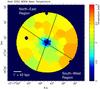 |
Fig. 1 Mean temperature map derived from wdem fits to all spectra extracted from the bins in the picture above. The temperatures vary from 2 keV in the core up to 3.6 keV in the outer parts of the cluster. The error on the temperature in the majority of the bins is less than 10%. In the core, a star symbol marks the centre of the main cD galaxy. The areas indicated by the thick lines are the regions used to compare the radial profiles in the Northern-Eastern and South-Western parts of the cluster. |
4. Results
In Figs. 1, 2, 5, and 6, we show maps based on a wdem fit to the data with the low-temperature cut-off (β) fixed to 0.1. A multi-temperature model is needed, because a single temperature model does not provide an acceptable fit to the spectra extracted near the centre of the cluster. Assuming single-temperature gas, we find typical reduced C-statistic values in the central region that are of the order of 3 times the d.o.f. Maps using single-temperature models have been created, but they show unphysical structure in the pressure map. Therefore, we only show the maps extracted from multi-temperature fits.
The weighted mean temperature of the best-fit wdem distribution, is shown in Fig. 1. The temperature ranges from about 2 keV in the centre of the cluster up to 3.6 keV at a radius of ~3.5′. This trend in temperature is typical for a cooling-core cluster. Interestingly, the map shows the presence of an asymmetry in temperature. A large area toward the South-West of the cluster has a significantly lower temperature with respect to the gas in the other directions. This area is approximately 120 × 120 kpc in size and the map suggests it extends to a distance of about 2.5′ from the cluster centre.
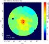 |
Fig. 2 Iron abundance map with respect to the proto-solar abundances by Lodders (2003). Uncertainties on the abundance values range from 5% in the centre up to 10% in the outer parts. In the core, a star symbol marks the centre of the main cD galaxy. |
Also the iron abundance map in Fig. 2 shows a similar asymmetry. Like other cooling-core clusters, the iron abundance is peaked in the centre. In the case of Abell 2052, the iron abundance reaches a peak value of about 1.2 times solar in the centre and drops off to about 0.5 solar at a distance of 4′ from the core. In the same South-Western region where the map in Fig. 1 shows lower temperatures, the iron abundance is relatively high. In this region, typical iron abundances are around 0.75 times solar, while on the opposite side of the cluster they are around 0.55 times solar.
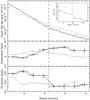 |
Fig. 3 Mean count rate per pixel, temperature, and iron abundance profiles extracted from the cool South-Western region (black) and the opposite North-Eastern side (gray) of Abell 2052. The upper panel shows the count rate as a function of the distance toward the central cD galaxy in the 0.5–10.0 keV band. The inset is a blow-up of the same data around the surface-brightness discontinuity. The second and third panel show the profiles of the temperature and iron abundance respectively. The dashed vertical line indicates the position of the surface brightness discontinuity. |
In order to see whether this area showing lower temperatures and high iron abundance is bound by a discontinuity, we extract a profile of the count rate in the direction of the asymmetry. The region from which we extract the count rates is the South-Western pie shaped region in Fig. 1. We bin the count-rates obtained from each image pixel into 0.1′ bins and the distance is chosen to be the radial distance toward the central cD galaxy. The count-rate profile is shown in the upper panel of Fig. 3. Indeed the profile is showing a jump around 3.2′. The inset in the upper panel of Fig. 3 shows a blow-up of this jump, which is not seen in the count rates determined from the opposite side of the cluster, which are shown in gray.
More detailed properties of the gas around the discontinuity are derived from spectra extracted from 0.5′ wide partial annuli. We extract spectra from eight partial annuli confined by the pie shaped region shown in Fig. 1 with radii ranging from 1.2–5.2′ with respect to the central cD galaxy. In the two lower panels of Fig. 3, we show the obtained temperature and iron abundance profiles from this region. For comparison, we also show these values for similar regions on the opposite side of the core, which are shown in gray. The position of the jump in count rate is indicated by the dashed vertical line. The temperature profiles confirm the asymmetry between the South-Western and North-Eastern region of the cluster. However, the profile does not show a jump at the radius of the surface-brightness discontinuity. Instead, they show a steady but asymmetric temperature gradient. Interestingly, the radius where the temperature profiles of the two opposite parts cross each other is ~2.6′, which is the same as the radius where the two surface-brightness profiles cross. The most remarkable feature is the jump in iron abundance at 3.2′. The abundance drops from ~0.75 to ~0.5 with respect to solar abundance units, which is consistent with the iron abundance values obtained from the maps. The area on the opposite side of the cluster, however, does not show a jump at that radius.
4.1. Density, entropy, and pressure
From the fits, we can calculate thermodynamic properties of the gas like entropy and pressure. If the surface-brightness discontinuity we found in the South-West of the cluster is a shock, then we expect, for example, that the entropy increases after the shock has passed. For a cold front, the contrary is expected. Then the entropy would be lower on the inner side of the discontinuity. Since the entropy and pressure are calculated from the electron temperature and density of the gas, the density needs to be derived first. This is calculated using the normalisation (Y) of the wdem component, which is given by  , where nH is the hydrogen density, ne is equal to 1.2nH for Solar metalicity, and V is the volume. In order to estimate the density for the annuli, we have to assume a size for the partial annulus along the line of sight to determine the volume. We choose this distance to be linearly proportional to the radius and in absolute value similar to the width of the partial annulus. The resulting density profile is shown in the top panel of Fig. 4. The plot shows that the density is smoothly decreasing outwards. Around the discontinuity, the density is slightly lower than in a reference region on the other side of the cluster, shown in gray. However, this plot does not show a discontinuity in density around 3′.
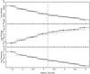 |
Fig. 4 Profiles of the derived density (m-3, upper panel), entropy (N m3, middle panel), and pressure (N m-2, lower panel) from the cool South-Western region (black) and the opposite North-Eastern side (gray) of Abell 2052. The dashed vertical line indicates the position of the surface brightness discontinuity. |
Using this density profile, we can calculate the pseudo entropy following the equation  , where S is the (pseudo) entropy, k is the Boltzmann constant, T is the temperature, and ne is the electron density. The entropy profile is shown in the middle panel of Fig. 4. A comparison between the profile around the discontinuity and the profile on the other side of the cluster shows that the entropy is also asymmetric. However, no strong entropy jump is seen around 3.2′. The asymmetry is also present in the entropy map shown in Fig. 5. For these maps, the probed volume is estimated in a slightly different way compared to the profiles in Fig. 4. We use the surface area of the bin in kpc2 times a typical constant depth of 200 kpc. Then, of course, we neglect the slight dependence of the volume with radius. But since we are mainly interested in the relative differences, this dependence is not important for this discussion. The asymmetry shown in the entropy map appears to be much smoother than the structure seen in the temperature and iron abundance maps. The fact that the entropy is lower in the inner region with respect to the discontinuity suggests that the discontinuity is a cold front.
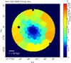 |
Fig. 5 Entropy map showing the (pseudo) entropy values, derived using the temperature and density estimates obtained from the spectral fits. In the core, a star symbol marks the centre of the main cD galaxy. |
Finally, we can also derive the spatial profile of the pressure, which is shown in the lower panel of Fig. 4. The pressure is calculated using P = nekT. The profiles of both sides of the cluster are very similar and smoothly decreasing outwards. Also the pressure map, which is not shown here, shows no significant asymmetries. There are no discontinuities seen around 3.2′, which suggest that the velocity of the front is low.
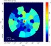 |
Fig. 6 Map of the value of the α parameter in the wdem model with β fixed to 0.1. The higher the α parameter, the higher the relative contribution of cooler components in the spectrum. The error on the α parameter is less than 30% across the image, except for the bins where the value of α is nearly zero. These bins are within 2σ significance consistent with their neighbours which have higher α values. In the central region, the typical uncertainty is less than 10%. In the core, a star symbol marks the centre of the main cD galaxy and the white arrow points out the bins with the highest α value. |
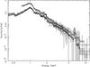 |
Fig. 7 EPIC MOS and pn spectra for AO1 and AO4 extracted from the North-Western region, which shows the low-temperature cut-off of ~0.5 keV. The data and best-fit model both represent the total spectrum including all the cosmic and instrumental background components. The models start diverging above 8 keV, because the instrumental background starts to dominate in this energy band. |
Best-fit results for the multi-temperature fitting of the region with the high-alpha parameter.
4.2. Multi-temperature regions
Since we used a multi-temperature wdem model to fit the spectra from the maps, there is also an estimate for the slope of the DEM distribution α. In Fig. 6, we show a map of α with β fixed to 0.1. A value near zero means that the DEM distribution is very peaked (near single-temperature), and a value significantly larger than zero means that there is a significant contribution of low-temperature gas. Surprisingly, there is a small region in the cluster with a large value for α, which is located just to the North-Western side of the central galaxy. This region is indicated with an arrow in Fig. 6. The maximum value for α is 1.06 ± 0.09, while the values in the immediate surroundings are typically 0.3. The large value suggests a large contribution of a cool component.
These bins that have an unusually high α value are associated with a very interesting multi-temperature region. Therefore, we extract a spectrum from a circular region centered on the bin with the high α value. The resulting spectra for EPIC MOS and pn are shown in Fig. 7. The radius of the extraction region is 15′′. We attempt to put constraints on the DEM distribution by fitting six empirical DEM distributions to the spectrum, which we explain in Sect. 3. The results of the fits are listed in Table 3. Although there are some variations, the best-fit C-statistic values for the multi-temperature fits are very similar. The iron abundances that we derive from the multi-temperature models are typically around 1.25 solar, except for the logarithmic Gaussian DEM model, which gives a lower iron abundance of 1.14 ± 0.02. In general, the derived mean temperatures and iron abundances are almost the same regardless of the used multi-temperature model. However, this does not hold for a single-temperature model. A single-temperature fit to this region results in an unacceptable C-stat value of 2795/942 d.o.f. The temperature and iron abundance values are unrealistically low compared to the multi-temperature results. Therefore, we ignore this model in the discussion about the temperature structure of this region.
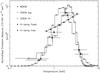 |
Fig. 8 Overview of the best-fit DEM distributions fitted to the North-Western multi-temperature region. The emission measure is normalised based on the width of the temperature bin. For the 4-temperature models, the bin width is somewhat arbitrary. We choose asymmetric bin sizes to form a continuous region from 0.5 up to 4 keV. |
The multi-temperature distributions that we fit are best compared by plotting them. In Fig. 8, we plot the DEM distributions and normalisations of five multi-temperature models. In this plot, the emission measures are normalised using the bin width to be able to compare them directly. Since the best-fit models have similar C-statistic values, the exact shape of the DEM distribution is uncertain. However, they all show a similar trend. The peak temperature of the distribution is found around temperatures of 2 and 3 keV. Above 3 keV, the contribution of high temperatures drops rapidly. Below 2 keV all models show a significant contribution of cool gas even down to 0.5 keV. Interestingly, the four-temperature models show an emission measure distribution that is comparable to the Gaussian DEM models.
Using the 4-temperature model with the fixed temperatures, we estimate the volume-filling fractions of the temperature components if we assume that the gas is in pressure equilibrium. For component i of n temperature components, the volume filling fraction (fi) for a multi-phase gas is given by (Sanders et al. 2004): 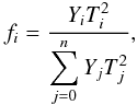 (2)where Yi is the emission measure and Ti the temperature of the ith component. For the 0.5 keV component of the 4-temperature model with the fixed kTmax of 4.0 keV, we find a volume filling fraction f of (1.02 ± 0.09) × 10-3 and for the 1.0 keV component we find (2.83 ± 0.17) × 10-2. In other clusters, these fractions are typically of the order of 10-3 and 10-2 for temperatures of 0.5 and 1.0 keV, respectively. Fractions of this order have been measured in, for example, Abell 3281 (Sanders et al. 2010) and M 87 (Werner et al. 2010).
We checked the spectrum for the presence of a cool 0.2 keV component and find a one sigma upper limit for the emission measure of Y < 2.5 × 1069 m-3. In principle, this measurement may be slightly biased due to the Galactic background components that have similar temperatures. However, these background components have an order of magnitude lower emission measure (Y ~ 1068 m-3) if they were placed at the cluster redshift. Since we fix the background to the emission measures we found in the outer parts of the cluster, the upper limit is robust.
5. Discussion
In the maps derived from XMM-Newton EPIC data of Abell 2052, we find two striking features in addition to what was already known about the cluster structure from detailed Chandra observations (Blanton et al. 2001, 2003, 2009). To the South-West of the cluster there is a large region with a relatively low entropy and temperature, but with a higher iron abundance. The Southern border of the region is formed by a surface brightness discontinuity. Just North-West of the central galaxy, we find a smaller region, which shows an unusually high contribution of cool (0.5 keV) gas. We focus the discussion on these two findings.
5.1. The origin of the Southern asymmetry
Asymmetries in the temperature, entropy and abundance maps like we see to the South-West of the core of Abell 2052 are fairly common in clusters of galaxies. Usually, these low-temperature regions, or cold fronts, are confined by a sharp surface brightness discontinuity (see Markevitch & Vikhlinin 2007, for a review). For Abell 2052, Blanton et al. (2009) already describe the elliptical shape of inner the core in the North-South direction. But just outside the region with the X-ray cavities, the core shows ellipticity in the NE-SW direction with an enhanced surface brightness area in the South-West. This NE-SW ellipticity is seen in both XMM-Newton and Chandra images. A sharp discontinuity, however, is not seen directly in the current images. By extracting a radial profile for a pie shaped region in the South, we do see a discontinuity in the mean count rate at an angular distance of 3.2′ from the central cD galaxy.
The ellipticity of the low-temperature region, the relatively weak discontinuity at the edge, and no evidence for structure in the pressure map or pressure profile suggest that the asymmetry is not due to a recent large merger event. Also the cooling core is not disrupted, which means that the cause of the disruption was either weak or a long time ago. The fact that we see only a significant jump in surface brightness and Fe abundance across the discontinuity most likely indicates gas sloshing (Markevitch et al. 2001). In this case, a small merger event or a larger merger in the distant past caused the dark matter and the associated cool gas to oscillate in the gravitational potential of the cluster. We only observe a gradual temperature, density, entropy, or pressure gradient across the cold front, and the entropy on the inside of the discontinuity is lower than on the outside. This means that the velocity of the front must be subsonic, and the discontinuity is not a shock.
Contrary to the lack of significant thermodynamic discontinuities found in the profiles, the iron abundance jumps down roughly 0.2 solar units across the front. Numerical simulations show that sloshing motions can indeed cause discontinuities in abundance profiles (Ascasibar & Markevitch 2006). This jump in iron abundance suggests that the sloshing motions are a mechanism to transport low-entropy metal-rich gas to the outer parts of the cluster. Recently, the same effect has also been observed in M 87 (Simionescu et al. 2010). The fact that metal transport is observed in these deep observations of clusters of galaxies suggests that gas sloshing is generally a very important and a dominating effect in the transport of metals to the outer parts of clusters.
It is interesting that the discontinuity in the iron abundance is very sharp, while the temperature profile changes more gradually. This has not only been observed in Abell 2052, but, for example, also in M 87 (Simionescu et al. 2010). The general shape of the surface brightness, temperature, and iron abundance profiles in Abell 2052 look remarkably similar to those observed in M 87. The shape suggests that conduction may play a larger role than previously thought. Earlier observations have shown that conduction should be suppressed across cold fronts (Ettori & Fabian 2000; Markevitch & Vikhlinin 2007) likely due to the presence of magnetic fields parallel to the front. However, when a cold front ages, thermal conduction between the cool and hot gas may gradually smooth the temperature jump without affecting the jump in metalicity. Therefore, conduction appears to be more important than, for example, mixing, which would also smooth the metalicity jump.
In numerical simulations of cold fronts, often more than one cold front is seen on both sides of the cluster (e.g. Tittley & Henriksen 2005). If there are more then one, they are expected to alternate on an axis through the centre of the cluster. In Abell 2052, the counterpart of the front at 3.2′ may lie North-East of the centre. Blanton et al. (2009) identified two jumps in surface brightness in that area using a deep Chandra image. The locations of these jumps are indicated in Fig. 9. They are located at 45′′ and 67′′ from the cluster centre. The 67′′ jump may be the counterpart of the cold front at 3.2′. If we look back to Fig. 3, then the iron abundance profile of the NE side of the central galaxy shows a jump around 1.7′. Probably, this jump is a bit too far from the jumps identified in the Chandra data to be associated with the counterpart of the cold front we find, although the spatial resolution of our iron abundance profile is relatively low. In addition, this North-Eastern region may be affected by the AGN activity in the core of the cluster. However, the position of the NE jumps in surface brightness and iron abundance appear to support the core oscillation interpretation.
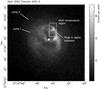 |
Fig. 9 Chandra ACIS-S image of Abell 2052. The bright point source in the centre is associated with the 3C 317 radio source. The image was smoothed using a Gaussian with a σ of 2 pixels. The box in the image indicates the region with a high wdem α parameter. In addition, we indicate a local peak of Hα+N ii emission (Baum et al. 1988). On the North-Eastern side, we indicate to surface brightness jumps identified by Blanton et al. (2009). |
5.2. Cool multi-temperature gas and Hα emission
In the map showing the slope of the DEM distribution, we find a small region North-West of the central galaxy that shows a relatively large contribution of cool gas. This region, with approximate dimensions of 10 × 20 kpc, is indicated on an archival Chandra ACIS-S image of Abell 2052 in Fig. 9. It coincides with a relatively bright spur of X-ray emission (Blanton et al. 2001). We fit the multi-temperature region North-West of the central galaxy with several multi-temperature models featuring different assumptions for the DEM distribution. From the C-statistic values it is clear that single-temperature models are inadequate to describe the observed spectrum, especially the temperature sensitive Fe-L complex. The underlying temperature structure is however difficult to constrain with the current instrumentation. Kaastra et al. (2004b) already show that spectra calculated from different DEM distributions with the same emission weighted average temperature and emission measure are almost indistinguishable at low spectral resolution. It is therefore not very surprising that we find similar C-statistic values for the wdem, gdem, and 4-temperature fits.
Although the exact shape of the DEM distribution cannot be derived, the global trends are quite robust. We can conclude from Fig. 8 that there is a significant amount of cool gas with temperatures of about 0.5–1.0 keV. The 1 keV component has about half of the emission measure with respect to the peak component of about 2.0 keV and the 0.5 keV component still has an emission measure between 10–20% of the peak component. Like in other clusters (e.g. Sanders et al. 2010), there appears to be a large drop in emission measure below a temperature of 0.5 keV. With the wdem model, we fit this low-temperature cut-off βkT and find values consistent with temperatures in the range of 0.5–0.6 keV. In addition, we find a one σ upper limit for the emission measure for a 0.2 keV component of Y < 2.5 × 1069 m-3, which is < 1.1% of the total emissivity. For a cooling-flow model with a mass deposition rate of 8 M⊙/yr, based on the 0.5 and 1.0 keV emission, an emission measure of Y ~ 1070 m-3 would be expected. This suggests that a physical mechanism should be at work at temperatures lower than 0.5 keV to prevent the gas from cooling radiatively.
Comparing this low-temperature cut-off directly with other clusters is not trivial, because for spectra with low-statistics, α and β are correlated. In previous papers the β parameter in the wdem model was often fixed to a low value (e.g. 0.1kTmax). A large contribution of cool gas is then indicated by a large value of α, which means a rather flat temperature distribution down to low temperatures. If we compare the value for α derived from our wdem fit to values found in the core regions of other clusters, then our value of 1.14 ± 0.05 is relatively high. In the cluster sample of Kaastra et al. (2004a), the values in the inner annuli are typically varying between 0.2–0.8, with the exception of Abell 1835 which shows an α value of 1.3 ± 0.5. Another example of a high α value of 1.1 ± 0.3 was found by de Plaa et al. (2004) in the central region of Abell 478, which also shows evidence of central AGN activity, like Abell 2052. The error bars on these measurements, however, are relatively large and the extraction regions of the spectra were not selected based on an α map. More recently, high α regions were found just to the east of M 87 (Simionescu et al. 2008). There are just a few bins in the α map that are larger than 1, which is similar to the situation in Abell 2052. Since Simionescu et al. (2008) leave the low-temperature cut-off (β) free, directly comparing absolute values of α is not possible. Relative differences in maps should, however, not be affected.
Detailed multi-wavelength studies of M87 show that these coolest regions are associated with Hα filaments (Young et al. 2002; Sparks et al. 2004; Werner et al. 2010). Similar regions were also found in other bright cool-core clusters or galaxies like, for example, Perseus (Fabian et al. 2003; Sanders & Fabian 2007), Centaurus (Crawford et al. 2005), and 2A 0335+096 (Sanders et al. 2009). In the multi-temperature region of Abell 2052, there is also a correlation between high α values and Hα emission. Hα data (Baum et al. 1988) overlaid on Chandra images (Blanton et al. 2001) show that the region where we find the high α values are also showing enhanced Hα+N ii emission. The peak of the Hα+N ii emission is exactly centered on the region with the enhanced cool components, within the resolution of our map. The Hα data of Baum et al. (1988) suggest that the blob of cool (T ~ 104 K) gas has been uplifted or pushed up by the Northern bubble, because there is a small filament of Hα emission extending from the central galaxy toward the North-Western blob. The Chandra image suggests that the region may be squeezed by the Northern large bubble, therefore increasing its density, and shorten its cooling time. Assuming pressure equilibrium, the radiative cooling time of the 0.5 keV gas in this region would be ~4 × 10⁶ yr. At this position, the blob is able to cool efficiently without being subsequently accreted or heated by the AGN. The only feedback mechanism that could heat the gas would be supernovae originating from star forming induced by continued gas cooling. Star formation is detected in optical and UV-images of the central cD galaxy, but it has not been reported at the position of this Hα spur (Martel et al. 2002; Blanton et al. 2003). In order to constrain the star formation rate due to gas cooling at the position of the spur, we searched for UV emission of young stars using data from the Optical Monitor (OM) aboard XMM-Newton. In a 29 ks OM exposure using the UVW1 filter, we also do not detect enhanced UV emission at this position. From the data, we derive a one sigma upper limit for the UV luminosity of a possible star forming region of L = 1.21 × 10¹⁸ W Hz-1. This would roughly correspond to a star formation rate of 1.7 × 10⁻³ M⊙/yr (Kennicutt 1998), which means that the gas does not continue cooling to star-forming temperatures.
It is still unclear how the brightness of the optical Hα emission can be explained. For the small sample of Sanders et al. (2010), the Hα luminosities in these regions are comparable or even higher than the missing X-ray luminosity below 0.5 keV (~1035 W s-1). Most likely, the Hα emission is concentrated in thin filaments (Sharma et al. 2010) embedded in the hotter 0.5 keV gas. The volume filling fraction of 1.1 × 10⁻³ for the 0.5 keV component would support the clumpy or filamentary nature of this gas. Since gas cooler than 0.5 keV is not detected in X-rays, the 0.5 keV gas is probably cooling non-radiatively. Fabian et al. (2002) suggest that heat is transferred from the 0.5 keV gas to the Hα emitting gas through mixing or conduction. Since the Hα emitting gas is probably magnetised, conduction and mixing may not be fully responsible for heating the Hα gas. Fabian et al. (2008) and Ferland et al. (2009) show that magnetic fields in these filaments can be relatively strong.
Small MHD shocks or waves may also play a role in mixing the coolest X-ray and cold Hα gas phases. Werner et al. (2010) propose that passing shock waves can accelerate the ICM past the much denser Hα filaments, which induces shearing and subsequently Kelvin-Helmholtz instabilities that mix the two phases. The hot ICM electrons then ionize and heat the cool gas, which induces Hα emission. Shocks and sound waves have been seen in recent Chandra observations of Abell 2052 (Blanton et al. 2009). Chandra images show a lot of smaller shock fronts or sound waves around the edges of the bubbles, and also just in front of the blob of Hα emission. Werner et al. (2010) base this hypothesis on the fact that most Hα regions are seen in the downstream regions of a shock. Therefore, this mechanism could explain why the X-ray gas would cool non-radiatively below 0.5 keV. Mixing and shock heating may also explain why the gas does not cool all the way to star-forming temperatures. Since observations of M87, for example, have shown that the Hα filaments contain dust (Sparks et al. 1993), the shocks should just gently heat the gas and not evaporate the dust. The multi-temperature region of Abell 2052 appears to be fully consistent with the Hα and 0.5 keV gas interactions as seen in M 87. However, in a recent Hα survey of 23 clusters (McDonald et al. 2010), Abell 2052 is one of few objects where the NUV/Hα flux ratio is consistent with shock heating. Therefore, this region may prove to be a very interesting special case. More detailed Hα, CO, UV measurements are necessary to unravel the heating and feedback mechanisms operating in this filament.
6. Conclusions
Using a deep XMM-Newton observation (95 ks), we have derived 2D maps of the core of the cluster Abell 2052. In the maps, we discover a cold front at a distance of ~130 kpc in the South-Western direction from the central cD galaxy. Close to the cD galaxy in the North-Western direction, we find a multi-temperature region with cool X-ray emitting gas as low as 0.5 keV. From a careful analysis of these regions, we conclude that:
-
We find a small local cooling-flow region NW of the cD galaxy. Most likely, this gas has been uplifted or pushed away from the core and squeezed by a nearby bubble, where it can cool efficiently and relatively undisturbed.
-
In the cooling-flow region NW of the cD galaxy, we do not detect gas below 0.5 keV. Although we cannot constrain the shape of the Differential Emission Measure distribution, the upper limit for gas around 0.2 keV is robust and lower than the emission measure expected from cooling-flow models.
-
The lack of lines from gas below 0.5 keV may be explained by the presence of Hα filaments. Shock induced mixing between the two phases may cause the 0.5 keV gas to cool non-radiatively.
-
We find significant jumps in surface brightness and iron abundance across the cold front in the South-Western part of the cluster, but no indications for a high Mach number. Therefore, it is a cold front and most likely the result of gas sloshing.
-
The sharp jump in iron abundance across the cold front suggests that sloshing is at least partly responsible for transporting metals from the core region to the outer parts of the cluster. In addition, the smooth temperature profile in the same area as the sharp iron jump suggests that conduction is responsible for smoothing the temperature gradient instead of mixing.
Acknowledgments
This work is based on observations obtained with XMM-Newton, an ESA science mission with instruments and contributions directly funded by ESA Member States and NASA. The Netherlands Institute for Space Research (SRON) is supported financially by NWO, the Netherlands Organisation for Scientific Research. N. Werner and A. Simionescu were supported by the National Aeronautics and Space Administration through Chandra/Einstein Postdoctoral Fellowship Award Numbers PF8-90056 and PF9-00070 issued by the Chandra X-ray Observatory Center, which is operated by the Smithsonian Astrophysical Observatory for and on behalf of the National Aeronautics and Space Administration under contract NAS8-03060.
References
- Ascasibar, Y., & Markevitch, M. 2006, ApJ, 650, 102 [NASA ADS] [CrossRef] [Google Scholar]
- Bîrzan, L., Rafferty, D. A., McNamara, B. R., Wise, M. W., & Nulsen, P. E. J. 2004, ApJ, 607, 800 [NASA ADS] [CrossRef] [Google Scholar]
- Baum, S. A., Heckman, T. M., Bridle, A., van Breugel, W. J. M., & Miley, G. K. 1988, ApJS, 68, 643 [NASA ADS] [CrossRef] [Google Scholar]
- Blanton, E. L., Sarazin, C. L., McNamara, B. R., & Wise, M. W. 2001, ApJ, 558, L15 [NASA ADS] [CrossRef] [Google Scholar]
- Blanton, E. L., Sarazin, C. L., & McNamara, B. R. 2003, ApJ, 585, 227 [NASA ADS] [CrossRef] [Google Scholar]
- Blanton, E. L., Randall, S. W., Douglass, E. M., et al. 2009, ApJ, 697, L95 [NASA ADS] [CrossRef] [Google Scholar]
- Brüggen, M., & Kaiser, C. R. 2002, Nature, 418, 301 [NASA ADS] [CrossRef] [PubMed] [Google Scholar]
- Cappellari, M., & Copin, Y. 2003, MNRAS, 342, 345 [NASA ADS] [CrossRef] [Google Scholar]
- Churazov, E., Sunyaev, R., Forman, W., & Böhringer, H. 2002, MNRAS, 332, 729 [NASA ADS] [CrossRef] [Google Scholar]
- Crawford, C. S., Hatch, N. A., Fabian, A. C., & Sanders, J. S. 2005, MNRAS, 363, 216 [NASA ADS] [CrossRef] [Google Scholar]
- De Luca, A., & Molendi, S. 2004, A&A, 419, 837 [NASA ADS] [CrossRef] [EDP Sciences] [Google Scholar]
- de Plaa, J., Kaastra, J. S., Tamura, T., et al. 2004, A&A, 423, 49 [NASA ADS] [CrossRef] [EDP Sciences] [Google Scholar]
- de Plaa, J., Kaastra, J. S., Méndez, M., et al. 2005, Adv. Space Res., 36, 601 [NASA ADS] [CrossRef] [Google Scholar]
- de Plaa, J., Werner, N., Bykov, A. M., et al. 2006, A&A, 452, 397 [NASA ADS] [CrossRef] [EDP Sciences] [Google Scholar]
- de Plaa, J., Werner, N., Bleeker, J. A. M., et al. 2007, A&A, 465, 345 [NASA ADS] [CrossRef] [EDP Sciences] [Google Scholar]
- den Herder, J. W., Brinkman, A. C., Kahn, S. M., et al. 2001, A&A, 365, L7 [NASA ADS] [CrossRef] [EDP Sciences] [Google Scholar]
- Diehl, S., & Statler, T. S. 2006, MNRAS, 368, 497 [NASA ADS] [CrossRef] [Google Scholar]
- Ettori, S., & Fabian, A. C. 2000, MNRAS, 317, L57 [NASA ADS] [CrossRef] [Google Scholar]
- Fabian, A. C. 1994, ARA&A, 32, 277 [NASA ADS] [CrossRef] [Google Scholar]
- Fabian, A. C., Allen, S. W., Crawford, C. S., et al. 2002, MNRAS, 332, L50 [NASA ADS] [CrossRef] [Google Scholar]
- Fabian, A. C., Sanders, J. S., Crawford, C. S., et al. 2003, MNRAS, 344, L48 [NASA ADS] [CrossRef] [Google Scholar]
- Fabian, A. C., Johnstone, R. M., Sanders, J. S., et al. 2008, Nature, 454, 968 [NASA ADS] [CrossRef] [PubMed] [Google Scholar]
- Ferland, G. J., Fabian, A. C., Hatch, N. A., et al. 2009, MNRAS, 392, 1475 [NASA ADS] [CrossRef] [Google Scholar]
- Finoguenov, A., Arnaud, M., & David, L. P. 2001, ApJ, 555, 191 [NASA ADS] [CrossRef] [Google Scholar]
- Giacconi, R., Murray, S., Gursky, H., et al. 1972, ApJ, 178, 281 [NASA ADS] [CrossRef] [Google Scholar]
- Heinz, C. J., Clark, G. W., Lewin, W. H. G., Schnopper, H. W., & Sprott, G. F. 1974, ApJ, 188, L41 [NASA ADS] [CrossRef] [Google Scholar]
- Kaastra, J. S., Mewe, R., & Nieuwenhuijzen, H. 1996, in UV and X-ray Spectroscopy of Astrophysical and Laboratory Plasmas. ed. K. Yamashita, & T. Watanabe (Tokyo: Universal Academy Press), 411 [Google Scholar]
- Kaastra, J. S., Ferrigno, C., Tamura, T., et al. 2001, A&A, 365, L99 [NASA ADS] [CrossRef] [EDP Sciences] [Google Scholar]
- Kaastra, J. S., Tamura, T., Peterson, J. R., et al. 2004a, A&A, 413, 415 [NASA ADS] [CrossRef] [EDP Sciences] [Google Scholar]
- Kaastra, J. S., Tamura, T., Peterson, J. R., et al. 2004b, in Proceedings of The Riddle of Cooling Flows in Galaxies and Clusters of Galaxies, held in Charlottesville, VA, May 31–June 4, 2003, ed. T. Reiprich, J. Kempner, & N. Soker, http://www.astro.virginia.edu/coolflow/ [Google Scholar]
- Kalberla, P. M. W., Burton, W. B., Hartmann, D., et al. 2005, A&A, 440, 775 [NASA ADS] [CrossRef] [EDP Sciences] [Google Scholar]
- Kennicutt, Jr., R. C. 1998, ARA&A, 36, 189 [Google Scholar]
- Kuntz, K. D., & Snowden, S. L. 2000, ApJ, 543, 195 [NASA ADS] [CrossRef] [Google Scholar]
- Kuntz, K. D., & Snowden, S. L. 2008, ApJ, 674, 209 [NASA ADS] [CrossRef] [Google Scholar]
- Lodders, K. 2003, ApJ, 591, 1220 [NASA ADS] [CrossRef] [Google Scholar]
- Markevitch, M., & Vikhlinin, A. 2007, Phys. Rep., 443, 1 [NASA ADS] [CrossRef] [EDP Sciences] [Google Scholar]
- Markevitch, M., Vikhlinin, A., & Mazzotta, P. 2001, ApJ, 562, L153 [NASA ADS] [CrossRef] [Google Scholar]
- Martel, A. R., Sparks, W. B., Allen, M. G., Koekemoer, A. M., & Baum, S. A. 2002, AJ, 123, 1357 [NASA ADS] [CrossRef] [Google Scholar]
- McDonald, M., Veilleux, S., Rupke, D. S. N., & Mushotzky, R. 2010, ApJ, 721, 1262 [NASA ADS] [CrossRef] [Google Scholar]
- McNamara, B. R., Wise, M., Nulsen, P. E. J., et al. 2000, ApJ, 534, L135 [CrossRef] [Google Scholar]
- Peterson, J. R., Paerels, F. B. S., Kaastra, J. S., et al. 2001, A&A, 365, L104 [Google Scholar]
- Peterson, J. R., Kahn, S. M., Paerels, F. B. S., et al. 2003, ApJ, 590, 207 [NASA ADS] [CrossRef] [Google Scholar]
- Sanders, J. S., & Fabian, A. C. 2002, MNRAS, 331, 273 [NASA ADS] [CrossRef] [Google Scholar]
- Sanders, J. S., & Fabian, A. C. 2007, MNRAS, 381, 1381 [NASA ADS] [CrossRef] [Google Scholar]
- Sanders, J. S., Fabian, A. C., Allen, S. W., & Schmidt, R. W. 2004, MNRAS, 349, 952 [NASA ADS] [CrossRef] [Google Scholar]
- Sanders, J. S., Fabian, A. C., & Taylor, G. B. 2009, MNRAS, 396, 1449 [NASA ADS] [CrossRef] [Google Scholar]
- Sanders, J. S., Fabian, A. C., Frank, K. A., Peterson, J. R., & Russell, H. R. 2010, MNRAS, 402, 127 [NASA ADS] [CrossRef] [Google Scholar]
- Sharma, P., Parrish, I. J., & Quataert, E. 2010, ApJ, 720, 652 [NASA ADS] [CrossRef] [Google Scholar]
- Simionescu, A., Werner, N., Finoguenov, A., Böhringer, H., & Brüggen, M. 2008, A&A, 482, 97 [NASA ADS] [CrossRef] [EDP Sciences] [Google Scholar]
- Simionescu, A., Werner, N., Forman, W. R., et al. 2010, MNRAS, 405, 91 [NASA ADS] [Google Scholar]
- Snowden, S. L., Mushotzky, R. F., Kuntz, K. D., & Davis, D. S. 2008, A&A, 478, 615 [NASA ADS] [CrossRef] [EDP Sciences] [Google Scholar]
- Sparks, W. B., Ford, H. C., & Kinney, A. L. 1993, ApJ, 413, 531 [NASA ADS] [CrossRef] [Google Scholar]
- Sparks, W. B., Donahue, M., Jordán, A., Ferrarese, L., & Côté, P. 2004, ApJ, 607, 294 [NASA ADS] [CrossRef] [Google Scholar]
- Tamura, T., Kaastra, J. S., Peterson, J. R., et al. 2001, A&A, 365, L87 [NASA ADS] [CrossRef] [EDP Sciences] [Google Scholar]
- Tamura, T., Kaastra, J. S., den Herder, J. W. A., Bleeker, J. A. M., & Peterson, J. R. 2004, A&A, 420, 135 [NASA ADS] [CrossRef] [EDP Sciences] [Google Scholar]
- Tittley, E. R., & Henriksen, M. 2005, ApJ, 618, 227 [NASA ADS] [CrossRef] [Google Scholar]
- Werner, N., de Plaa, J., Kaastra, J. S., et al. 2006, A&A, 449, 475 [NASA ADS] [CrossRef] [EDP Sciences] [Google Scholar]
- Werner, N., Simionescu, A., Million, E. T., et al. 2010, MNRAS, 407, 2063 [NASA ADS] [CrossRef] [Google Scholar]
- Young, A. J., Wilson, A. S., & Mundell, C. G. 2002, ApJ, 579, 560 [NASA ADS] [CrossRef] [Google Scholar]
- Zhao, J.-H., Sumi, D. M., Burns, J. O., & Duric, N. 1993, ApJ, 416, 51 [NASA ADS] [CrossRef] [Google Scholar]
All Tables
List of observation IDs used for the analysis with their useful exposure time in ks after flare filtering.
Best-fit results for the multi-temperature fitting of the region with the high-alpha parameter.
All Figures
|
Fig. 1 Mean temperature map derived from wdem fits to all spectra extracted from the bins in the picture above. The temperatures vary from 2 keV in the core up to 3.6 keV in the outer parts of the cluster. The error on the temperature in the majority of the bins is less than 10%. In the core, a star symbol marks the centre of the main cD galaxy. The areas indicated by the thick lines are the regions used to compare the radial profiles in the Northern-Eastern and South-Western parts of the cluster. |
| In the text | |
|
Fig. 2 Iron abundance map with respect to the proto-solar abundances by Lodders (2003). Uncertainties on the abundance values range from 5% in the centre up to 10% in the outer parts. In the core, a star symbol marks the centre of the main cD galaxy. |
| In the text | |
|
Fig. 3 Mean count rate per pixel, temperature, and iron abundance profiles extracted from the cool South-Western region (black) and the opposite North-Eastern side (gray) of Abell 2052. The upper panel shows the count rate as a function of the distance toward the central cD galaxy in the 0.5–10.0 keV band. The inset is a blow-up of the same data around the surface-brightness discontinuity. The second and third panel show the profiles of the temperature and iron abundance respectively. The dashed vertical line indicates the position of the surface brightness discontinuity. |
| In the text | |
|
Fig. 4 Profiles of the derived density (m-3, upper panel), entropy (N m3, middle panel), and pressure (N m-2, lower panel) from the cool South-Western region (black) and the opposite North-Eastern side (gray) of Abell 2052. The dashed vertical line indicates the position of the surface brightness discontinuity. |
| In the text | |
|
Fig. 5 Entropy map showing the (pseudo) entropy values, derived using the temperature and density estimates obtained from the spectral fits. In the core, a star symbol marks the centre of the main cD galaxy. |
| In the text | |
|
Fig. 6 Map of the value of the α parameter in the wdem model with β fixed to 0.1. The higher the α parameter, the higher the relative contribution of cooler components in the spectrum. The error on the α parameter is less than 30% across the image, except for the bins where the value of α is nearly zero. These bins are within 2σ significance consistent with their neighbours which have higher α values. In the central region, the typical uncertainty is less than 10%. In the core, a star symbol marks the centre of the main cD galaxy and the white arrow points out the bins with the highest α value. |
| In the text | |
|
Fig. 7 EPIC MOS and pn spectra for AO1 and AO4 extracted from the North-Western region, which shows the low-temperature cut-off of ~0.5 keV. The data and best-fit model both represent the total spectrum including all the cosmic and instrumental background components. The models start diverging above 8 keV, because the instrumental background starts to dominate in this energy band. |
| In the text | |
|
Fig. 8 Overview of the best-fit DEM distributions fitted to the North-Western multi-temperature region. The emission measure is normalised based on the width of the temperature bin. For the 4-temperature models, the bin width is somewhat arbitrary. We choose asymmetric bin sizes to form a continuous region from 0.5 up to 4 keV. |
| In the text | |
|
Fig. 9 Chandra ACIS-S image of Abell 2052. The bright point source in the centre is associated with the 3C 317 radio source. The image was smoothed using a Gaussian with a σ of 2 pixels. The box in the image indicates the region with a high wdem α parameter. In addition, we indicate a local peak of Hα+N ii emission (Baum et al. 1988). On the North-Eastern side, we indicate to surface brightness jumps identified by Blanton et al. (2009). |
| In the text | |
Current usage metrics show cumulative count of Article Views (full-text article views including HTML views, PDF and ePub downloads, according to the available data) and Abstracts Views on Vision4Press platform.
Data correspond to usage on the plateform after 2015. The current usage metrics is available 48-96 hours after online publication and is updated daily on week days.
Initial download of the metrics may take a while.