| Issue |
A&A
Volume 523, November-December 2010
|
|
|---|---|---|
| Article Number | A70 | |
| Number of page(s) | 21 | |
| Section | Interstellar and circumstellar matter | |
| DOI | https://doi.org/10.1051/0004-6361/200810340 | |
| Published online | 18 November 2010 | |
Photometry and spectroscopy of GRB 060526: a detailed study of the afterglow and host galaxy of a z = 3.2 gamma-ray burst⋆,⋆⋆
1
Dark Cosmology Centre, Niels Bohr Institute, University of
Copenhagen, Juliane Maries Vej
30, 2100
Copenhagen,
Denmark
e-mail: This email address is being protected from spambots. You need JavaScript enabled to view it.
2
INAF – Osservatorio Astronomico di Brera,
via Bianchi 46, 23807
Merate ( Lc), Italy
3
Thüringer Landessternwarte Tautenburg,
Sternwarte 5, 07778
Tautenburg,
Germany
4
Science Institute, University of Iceland,
Dunhaga 3, 107
Reykjavík,
Iceland
5
Hansen Experimental Physics Laboratory, Stanford
University, Stanford,
CA
94305,
USA
6
Institute of Theoretical Astrophysics, University of
Oslo, PO Box 1029
Blindern, 0315
Oslo,
Norway
7
Department of Physics, University of Michigan,
Ann Arbor, MI
48109,
USA
8
Physical Research Laboratory, Ahmedabad – 380 009, India
9
Dipartimento di Astronomia, Universita di Bologna,
via Ranzani 1, 40127
Bologna,
Italy
10
Kazan Federal University and Academy of Sciences of
Tatarstan, Kazan,
Russia
11
Department of Astronomy, 601 Campbell Hall, University of
California, Berkeley,
CA
94720–3411,
USA
12
Space Research Institute (IKI), 84/32 Profsoyuznaya Str, Moscow
117997,
Russia
13
Department of Astronomy, Yale University,
PO Box 208101, New Haven, CT
06520,
USA
14
Astronomical Institute “Anton Pannekoek”, University of
Amsterdam, Kruislaan
403, 1098 SJ
Amsterdam, The
Netherlands
15
Mullard Space Science Laboratory, University College
London, Holmbury St. Mary,
Dorking, Surrey
RH5 6NT,
UK
16
UCD School of Physics, University College Dublin,
Belfield, Dublin 4, Ireland
17
Max-Planck-Institute for Extraterrestrial Physics, Giessenbachstraße, 85748
Garching,
Germany
18
Space Telescope Science Institute, 3700 San Martin Drive, Baltimore, MD21218, USA
19
Ulugh Beg Astronomical Institute, 33 Astronomical Str., Tashkent
700052,
Uzbekistan
20
INAF – Osservatorio Astronomico di Roma, via Frascati 33,
00040
Monteporzio Catone,
Italy
21
Centre for Astrophysics and Cosmology, Science Institute,
University of Iceland, Dunhagi
5, 107
Reykjavík,
Iceland
22
Instituto de Astrofísica de Andalucía (IAA-CSIC),
PO Box 3.004,
18. 080
Granada,
Spain
23
Niels Bohr Institute, University of Copenhagen,
Juliane Maries Vej
30, 2100
Copenhagen,
Denmark
24
Centre for Star and Planet Formation, Geological Museum, Øster
Voldgade 5-7, 1350
Copenhagen,
Denmark
25
Tübitak National Observatory, Antalya, Turkey
26
Department of Astronomy and Astrophysics, Pennsylvania State
University, 525 Davey
Lab, University Park, PA
16802,
USA
27
Department of Physics, Univ. of Warwick, Coventry, CV4 7AL, UK
28
INAF – Istituto di Astrofisica Spaziale e Fisica Cosmica di
Bologna, via Gobetti
101, 40129
Bologna,
Italy
29
University of Helsinki Observatory, PO Box 14 ( Tähtitorninmäki), 00014, Finland
30
VU Institute of Theoretical Physics and Astronomy,
A. Gostauto 12,
01108
Vilnius,
Lithuania
31
Space Science Department, Southwest Research
Institute, San
Antonio, TX
78238,
USA
32
Steward Observatory, University of Arizona,
933 North Cherry
Avenue, Tucson,
AZ
85721,
USA
33
Crimean Astrophysical Observatory, Nauchny, Crimea, 98409,
Ukraine
34
Physics Department, University of California at Santa
Barbara, 2233B Broida
Hall, Santa
Barbara, CA
93106,
USA
35
Tabasgo Fellow, USA
36
Max-Plank-Institut für Astrophysik, Karl-Schwarzschild Straße 1, 85741
Garching,
Germany
37
Department of Physics and Astronomy, University of Leicester,
University Road, Leicester, LE1
7RH, UK
38
Second University of Roma “Tor Vergata”,
Italy
39
Department of Astronomy, University of Texas at
Austin, Austin
TX, 78712, USA
40
Department of Physics, College of St. Benedict/St. Johns
University, Collegeville, MN
56321,
USA
Received:
6
June
2008
Accepted:
17
July
2010
Abstract
Aims. With this paper we want to investigate the highly variable afterglow light curve and environment of gamma-ray burst (GRB) 060526 at z = 3.221.
Methods. We present one of the largest photometric datasets ever obtained for a GRB afterglow, consisting of multi-color photometric data from the ultraviolet to the near infrared. The data set contains 412 data points in total to which we add additional data from the literature. Furthermore, we present low-resolution high signal-to-noise spectra of the afterglow. The afterglow light curve is modeled with both an analytical model using broken power law fits and with a broad-band numerical model which includes energy injections. The absorption lines detected in the spectra are used to derive column densities using a multi-ion single-component curve-of-growth analysis from which we derive the metallicity of the host of GRB 060526.
Results. The temporal behaviour of the afterglow follows a double broken power law with breaks at t = 0.090 ± 0.005 and t = 2.401 ± 0.061 days. It shows deviations from the smooth set of power laws that can be modeled by additional energy injections from the central engine, although some significant microvariability remains. The broadband spectral-energy distribution of the afterglow shows no significant extinction along the line of sight. The metallicity derived from S ii and Fe ii of [S/H] = –0.57 ± 0.25 and [Fe/H] = –1.09 ± 0.24 is relatively high for a galaxy at that redshift but comparable to the metallicity of other GRB hosts at similar redshifts. At the position of the afterglow, no host is detected to F775W(AB) = 28.5 mag with the HST, implying an absolute magnitude of the host M(1500 Å) > –18.3 mag which is fainter than most long-duration hosts, although the GRB may be associated with a faint galaxy at a distance of 11 kpc.
Key words: gamma rays bursts: individual: GRB 060526 / galaxies: high-redshift / ISM: abundances
Based in part on observations obtained with the European Southern Observatory’s Very Large Telescope under proposals 077.D-0661 (PI: Vreeswijk) and 177.A-0591 (PI: Hjorth), as well as observations obtained with the NASA/ESA Hubble Space Telescope under proposal 11734 (PI: Levan).
Table 1 is only available in electronic form at http://www.aanda.org
© ESO, 2010
1. Introduction
Gamma-ray bursts (GRBs) and their afterglows offer a powerful tool to probe the high-redshift universe, both through photometry and spectroscopy. The standard fireball model of GRB afterglows (see Zhang 2007; Mészáros et al. 2006; Gehrels et al. 2009, for recent reviews on the topic) predicts a smooth temporal evolution, and the resulting afterglow light curve can be empirically described by a joint smoothly-broken power law, the so-called Beuermann equation (Beuermann et al. 1999). For many GRBs in the pre-Swift era, when temporally dense afterglow photometry was obtained, the afterglow evolution was found to be smooth as, e.g., in GRB 020813 (Laursen & Stanek 2003), GRB 030226 (Klose et al. 2004) and GRB 041006 (Stanek et al. 2005) (for the complete pre-Swift sample see Zeh et al. 2006). Out of the total sample of 59 afterglows of that paper, only four of the GRBs analysed showed significant deviations from the expected decay (though we note that about half of the 59 afterglows were not sampled well enough to allow any conclusions). One might be explained by microlensing (GRB 000301C, Garnavich et al. 2000) and another one by assuming an inhomogeneously emitting surface (GRB 011211, Jakobsson et al. 2004). The other two GRBs which are the only ones showing long-lasting strong deviations are GRB 021004 (e.g. de Ugarte Postigo et al. 2005, and references therein) and GRB 030329 (e.g. Lipkin et al. 2004, and references therein), which incidentally also have the densest optical monitoring.
With the launch of the Swift satellite and its rapid localization capabilities (Gehrels et al. 2004), the number of highly variable light curves has increased considerably, though there are still examples of very smooth light curves (e.g. that of GRB 080210, which showed a smooth behaviour with a high sampling rate of 1 s, A. De Cia, priv. comm.). Some light curves show small, achromatic bumps overlying the smooth power law decay (e.g., GRB 050502A, Guidorzi et al. 2005; GRB 061007, Mundell et al. 2007; GRBs 090323 and 090328, McBreen et al. 2010), early bumps with chromatic evolution (e.g., GRB 061126, Perley et al. 2008a; GRB 071003, Perley et al. 2008b), “steps” due to energy injection episodes (e.g., GRB 070125, Updike et al. 2008; GRB 071010A, Covino et al. 2008; GRB 080913, Greiner et al. 2009b, GRB 090926A, Rau et al. 2010; Cenko et al. 2010; Swenson et al. 2010) or powerful late-time rebrightenings of up to several magnitudes (e.g., GRB 050721, Antonelli et al. 2006; GRB 060206, Woźniak et al. 2006; Monfardini et al. 2006; Stanek et al. 2007; GRB 070311, Guidorzi et al. 2007; GRB 071003, Perley et al. 2008b). The early time domain, which can now be routinely accessed by rapid follow-up in the Swift era, has yielded more types of variability, like rising afterglows (e.g., GRB 060418, Molinari et al. 2007; GRB 060605, Ferrero et al. 2009; GRB 060607A, Nysewander et al. 2009, Molinari et al. 2007; GRB 081008, Yuan et al. 2010; see Oates et al. 2009; Rykoff et al. 2009, for further examples) and short-term variability directly linked to the prompt emission (e.g., GRB 041219A, Vestrand et al. 2005; Blake et al. 2005; GRB 050820A, Vestrand et al. 2006; GRB 080319B, Racusin et al. 2008; GRB 080129, Greiner et al. 2009a). In all these cases, dense photometric follow-up during the periods of variability was needed to characterize the phenomena involved.
In addition to their use in studying the GRB phenomenon itself, GRB afterglows can be used to study their galactic environment through absorption line spectroscopy of material in the line-of-sight towards the GRB. Above a redshift of around z ~ 0.2, resonant absorption lines from elements present in the interstellar medium (ISM) such as Mg, Zn, Fe, Si, C, and S are shifted into the optical regime and can be studied with ground-based telescopes. For 10 bursts between a redshift of z = 2 to 6, the metallicity along the line-of-sight in the galaxy could be obtained so far (e.g. Savaglio 2006; Fynbo et al. 2006; Price et al. 2007; Prochaska et al. 2007; Ledoux et al. 2009, and references therein). The values are usually below solar, but higher than for QSO absorbers at comparable redshifts, some of them even higher than theoretical limits for the formation of collapsars (Woosley & Heger 2006). The difference to QSO absorbers can be explained if GRB sightlines probe denser parts of the galaxy, or if GRBs reside in galaxies with higher masses and therefore higher metallicities (Fynbo et al. 2008; Pontzen et al. 2010). Both for QSO and GRB absorbers, there seems to be a metallicity evolution with redshift (Savaglio 2006; Fynbo et al. 2006; Price et al. 2007), although the slope is different for the two samples. GRB hosts seem to show a low extinction along the line-of-sight (Prochaska et al. 2007), however, relative abundances of heavier elements indicate that some of the ions must be depleted onto dust grains and the depletion pattern resembles the one found in the warm disc and halo of the Milky Way (MW; Savaglio 2006). How this can be explained together with the low extinction as also derived from the spectral energy distribution (SED) of the afterglow (Kann et al. 2006, 2010; Starling et al. 2007), is still an open question. One possible solution to this problem is destruction of the dust present in the line-of-sight by the GRB and afterglow radiation (e.g., Waxman & Draine 2000; Perna & Lazzati 2002), though no strong evidence has ever been found for this. Furthermore, there is clearly a strong observational bias involved, as those GRB afterglows with successful spectroscopy, especially in the case of high-resolution observations, are those which have only low extinctions and thus relatively bright afterglows (Fynbo et al. 2009; Kann et al. 2010), although rapid observations with large telescopes can achieve detailed spectroscopy of highly extinguished afterglows, as in the case of GRB 080607 (Prochaska et al. 2009; Sheffer et al. 2009; Fynbo et al. 2009).
GRB 060526 was detected by the Swift satellite on May 26.686458 (16:28:29.95 UT). The satellite slewed immediately to the burst, detecting both the X-ray and the optical afterglow (Campana et al. 2006a). The BAT instrument on Swift measured two emission episodes. The first one lasted 13.8 s and consisted of two FRED (fast rise exponential decay) peaks, followed by a second symmetric peak between 230 and 270 s (Campana et al. 2006b). The second peak was coincident with a giant X-ray flare followed by a softer flare at 310 s (Campana et al. 2006c) also detected in the v band by the UVOT telescope on-board Swift (Brown et al. 2006). The gamma-ray fluence was (4.9 ± 0.6) × 10-7 erg cm-2 during the first emission episode and (5.9 ± 0.6) × 10-7 erg cm-2 during the second, the peak flux of the second episode was however only half of the peak flux of the first one. The photon index of the two epochs changed from 1.66 ± 0.20 to 2.07 ± 0.18, thus showing the typical hard-to-soft evolution (Markwardt et al. 2006). The Watcher telescope provided the first ground based detection with R ≈ 15 mag (French & Jelínek 2006) 36.2 s after the trigger. ROTSE observations showed a plateau for several thousand seconds after the GRB onset (Rykoff et al. 2006). A redshift of z = 3.21 was determined by Berger & Gladders (2006) with the Magellan/Clay telescope. The brightness of the optical afterglow allowed for a dense monitoring which revealed a complex light curve structure including several flares (Halpern et al. 2006a,b) and a steepening attributed to a jet break (Thöne et al. 2006).
In this paper, we approach the analysis of GRB 060526 from two directions: Through modelling of the very detailed optical light curve and late optical imaging of the field to detect the host in Sect. 3, and analysis of low to medium resolution spectroscopic observations of absorption lines along the line of sight (Sect. 4). Throughout the paper, we follow the convention Fν(t) ∝ t−αν−β, and use WMAP concordant cosmology (Spergel et al. 2003) with H0 = 71 km s-1 Mpc-1, ΩM = 0.27, and ΩΛ = 0.73. Uncertainties are given at 68% confidence level for one parameter of interest unless stated otherwise.
2. Observations
2.1. Photometry
In order to get a good coverage of the light curve, we obtained data using several different telescopes around the world. Our complete data set comprises a total of 412 points from the UV to K-band, one of the largest photometric samples of an optical/NIR afterglow in the Swift era.
The earliest dataset was obtained by the Watcher telescope, located at Boyden Observatory, South Africa, starting 36.2 s after the burst, followed by Swift UVOT starting 86 s after the trigger. Early ground based optical data were obtained with the ROTSE-IIIc 0.3 m telescope at the HESS site at Mt. Gamsberg, Namibia, the 1.5 m telescope on Mt. Maidanak/Uzbekistan, the 2.6 m Shajn telescope at CrAO (Crimean Astrophysical Observatory/Ukraine), the TNG (Telescopio Nazionale Galileo) on La Palma equipped with DOLoRes, the 1.2 m MIRO telescope on Mt. Abu/India, with BFOSC (Bologna Faint Object Spectrograph & Camera) at the G. D. Cassini 152 cm telescope of the Bologna University under poor conditions and with the RTT150 (1.5 m Russian-Turkish telescope, Bakirlitepe, Turkey), the RTT150 data are also presented in Khamitov et al. (2007).
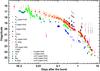 |
Fig. 1 Light curves of the optical afterglow of GRB 060526. Filled and open circles (detections, Bg′VRCCRICJHKS) and open triangles (upper limits, uvw2uvm2uvw1ubRCCRJHKS) are presented in this work, and open stars (Br′Ri′) are taken from Dai et al. (2007). The early light curve especially shows strong variability, with two flares seen in the UVOT v band data. The later light curve also shows evident variability, and the large V−R, B−R colours due to the high redshift are evident. Data in this plot are not corrected for foreground extinction. |
The light curve was followed up sparsely every night over nearly a week with DFOSC (Danish Faint Object Spectrograph and Camera) on the Danish 1.54 m telescope on La Silla/Chile under partially photometric conditions and with MOSCA (MOSaic CAmera) and ALFOSC (Andalucia Faint Object Spectrograph and Camera) at the Nordic Optical Telescope on La Palma. Furthermore, two epochs were obtained with the Tautenburg 1.34 m Schmidt telescope and two sets of images were taken several days after the GRB with Keck/LRIS simultaneously in the Kron-Cousins R and the Sloan g′ bands, the second observation was performed at high airmass under bad seeing conditions. Late images were obtained with FORS2 at the VLT on Paranal/Chile on Feb. 23, 2007 and Mar. 30, 2008 in the RC band with exposure times of 2500 and 7500 s, respectively, to look for the host galaxy. We also took observations with the Hubble Space Telescope on 9 August 2009, utilizing the Advanced Camera for Surveys with the F775W (roughly SDSS i′) filter (see Fig. 6). A total of 7844 s of observations were obtained in six dithered exposures. These were reduced via multidrizzle in the standard fashion.
Spectra of GRB 060526 from FORS1/VLT.
Near infrared data were collected with ANDICAM and the 1.3 m SMARTS telescope (Small and Moderate Aperture Research Telescope System) at CTIO under non-photometric conditions as well as with the robotic 1.3 m PAIRITEL telescope on Mt. Hopkins.
The UVOT data were reduced and analysed using the standard UVOT tasks within the heasoft package. For the photometric calibration of the ground-based data, we determined the calibrated magnitude of six comparison stars in the field using photometric zero points from DFOSC in the V, RC and IC bands (see Table 3). These stars were then used to perform relative Point-Spread Function (PSF) photometry to get the calibrated magnitude of the afterglow. For some of the late NOT images as well as the faint MIRO detections, though, we applied relative aperture photometry using a circle of 20 pixels diameter (and an annulus of 10 pixels for the sky). For the B-band, where no DFOSC data were available, we took zero points for only three comparison stars from the SDSS (see Table 3), converting them with the equations of Jester et al. (2005). g′ zero points were taken from the SDSS, and they are given as AB magnitudes. For the RTT 150 data, we used one USNO-B1 star as reference that was calibrated using Landolt standard stars. The results are in full agreement with the rest of the data set. The Watcher data were analysed using a dedicated photometry pipeline (Ferrero et al. 2010). The J, H and KS band data from SMARTS/ANDICAM and PAIRITEL were calibrated using three and ten nearby stars, respectively, from the 2MASS catalogue. For the H and KS band data, we used smaller apertures and applied aperture corrections to reduce the influence of the highly variable background.
All data and upper limits are given in Table 1, the data are not corrected for Galactic extinction. Note we give the g′ and HST F775W magnitudes in AB magnitudes. For the final light curve fitting, we add Br′RCi′ band data from Dai et al. (2007). We shift the B and RC band data of Dai et al. (2007) by 0.1 mag to bring it to our zero point. The multi-color light curves are shown in Fig. 1.
2.2. Spectroscopy
Spectra were obtained with FORS1/VLT on May 27 from 9 to 12 h after the burst. Four different grisms cover the wavelength range from 3650 to 9200 Å. For all four grisms a 1″̣0 slit was used which provides resolutions between 2.4 and 11.1 Å. Reduction, cosmic ray removal, extraction and wavelength calibration were performed using standard tasks in IRAF1. The final spectra were then normalised as no absolute flux calibration was needed. In order to improve the S/N, we combined the datasets taken with the same grism weighted with their variance. A summary of the spectroscopic observations is given in Table 2.
3. Prompt emission
Up to two hours after the burst, the light curve features an optical flare contemporaneous to the XRT/BAT flare at ≈ 250 s and a following plateau phase (Brown et al. 2006; French & Jelínek 2006; Rykoff et al. 2006). We reduced the BAT event data using standard procedures within the software provided by HEASOFT (version 6.1). The XRT observations were reduced using the standard xrtpipeline (version 0.10.4) for XRT data analysis software using the most recent calibration files. The spectral data of BAT and XRT were analysed with XSPEC version 11.3 (Arnaud 1996). The X-ray Galactic column density was fixed to 5.02 × 1020 cm-2 (Kalberla et al. 2005). We estimated the late-time extragalactic column density by fitting the XRT PC data from 517 s to 1.34 × 10⁵ s post trigger, where spectral evolution is negligible, using an absorbed power law model. We only find an upper limit of NHX < 9.8 × 1021 cm-2 (see also Campana et al. 2010).
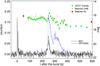 |
Fig. 2 The two early flares seen in the BAT and XRT data and temporally coincident optical observations by UVOT and Watcher. The second flare is much softer at high energies and hence it is only seen in the XRT data. Both flares are reflected in the optical data with the first optical flare being coincident with the first BAT/XRT flare while the second flare is delayed compared to the second X-ray flare. The white data have been shifted upward by 0.3 mag to the v zero point. A color version of the figure is available in the online version of the article. |
In Fig. 2 we compare the timescale of the flares at high energies (BAT and XRT) with contemporaneous optical data. The first, stronger flare is seen both by the XRT and BAT whereas the second, softer flare is only visible in the XRT data. Our earliest optical data are also coincident with the two flares. A broad early bump is observed in the optical light curve which precedes the second episode of BAT emission and the major X-ray pulse. The Watcher data only show a plateau during the high-energy flares due to a relatively low time resolution. The higher time-resolution of the UVOT data shows that there are also two significant flares in the optical. The first optical flare is contemporaneous with the peak of the BAT/XRT flare within 2σ of the temporal error. Then, there may also be a small optical bump (significance only ≈1.5σ) at the time of the second (XRT-only) flare, whereas the second significant optical flare occurs ≈90 s after the XRT-only flare implying that these two events are probably not connected. Power-law fitting of the optical light curve (with respect to the BAT trigger time T0) shows the slopes are very steep. The rising slope of the first flare is αr1 = −12.8 ± 3.0, and the decay slope is αd1 = 5.8 ± 0.8, or, if one takes the bump as a second flare, the two decay slopes are αd11 = 8.2 ± 2.0, αd12 = 8.6 ± 2.5. The rise and decay slopes for the second peak are similarly steep, but with larger uncertainties.
Prompt optical flashes attributed to reverse shocks, as seen in the landmark burst GRB 990123 (Akerlof et al. 1999), have been observed in only a few cases since the launch of Swift, e.g., GRB 060111B (Klotz et al. 2006) and GRB 060117 (Jelínek et al. 2006, see Kann et al. 2010 for a recent overview of light curves with probable reverse shock flashes/steep decays in the Swift era). Most bursts for which early optical data are available display no evidence of reverse shock emission. In a number of cases, the optical light curve is dominated by forward shock emission from very early times, e.g. GRB 050401 (Rykoff et al. 2005), GRB 060418 and GRB 060607A (Molinari et al. 2007; Nysewander et al. 2009), GRB 060605 (Ferrero et al. 2009), GRB 061007 (Mundell et al. 2007) and GRB 081008 (Yuan et al. 2010). An optical component of the emission from internal shocks has been invoked to explain the correlation between the optical and high-energy light curves observed in several bursts, e.g. GRB 041219A (Vestrand et al. 2005; Blake et al. 2005; Fan et al. 2005), GRB 050820A (Vestrand et al. 2006), and GRB 050904 (Wei et al. 2006). The very rapid variability as measured by the steep slopes and the contemporaneous first flare indicates that GRB 060526 is another case where the early optical light curve is dominated by central engine activity. Such time resolution and coincident optical and high-energy observations are still rare, however, a thorough analysis of the flares and their spectral properties goes beyond the scope of this paper.
Magnitudes of the comparison stars used for photometry.
4. Afterglow photometry and light curve modelling
4.1. The multi-color light curve
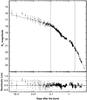 |
Fig. 3 The RC-band light curve of GRB 060526 fitted with a double smoothly-broken power law, using data starting at 0.046 days. The residuals of the fit show an early optical flare and later strong variations of up to 0.3 mag. The dashed vertical lines mark the break times, the dotted lines the 1σ region of uncertainty. The second break is soft (n ≈ 4) and is thus seen as a smooth rollover. |
To analyse the evolution of the light curve, we use the RC/CR band which has the densest sampling, a total of 319 data points in all, from 50 s to more than 7 days after the GRB. For all fits, we fix the host magnitude to mh = 29 (see Sect. 4.4). A fit with a single power law to these data is very strongly rejected, with χ2/d.o.f. = 31.89 (with 319 d.o.f.). Even if we remove the earliest data which are affected by optical flares, starting only at 400 s after the GRB, the fit is still rejected (χ2/d.o.f. = 29.46 with 308 d.o.f.). A double smoothly-broken power law gives a much better fit, but even so, the fit is formally rejected, with χ2/d.o.f. = 3.12 with 302 d.o.f. This is due to the strong variability in the light curve which was first found by Halpern et al. (2006a) and is also discussed in Dai et al. (2007). This fit, along with the residuals showing the strong variability, is shown in Fig. 3. The parameters we find for this fit (αplateau = 0.288 ± 0.026, α1 = 0.971 ± 0.008, α2 = 2.524 ± 0.052, tb1 = 0.090 ± 0.005 days, tb = 2.216 ± 0.049 days) are concurrent with those of Dai et al. (2007) (who find α1 ≈ 1.0, α2 ≈ 2.9 and tb ≈ 2.55 days).
Due to the high data density, we are able to let the break smoothness parameter n vary for the second break (the first break had to be fixed to n = 10), and our result (n = 4.3 ± 0.7) is in agreement with the tentative α1 − n correlation found by Zeh et al. (2006). Still, the significant improvement shows that the light curve is basically a double smoothly-broken power law, and the steep late decay indicates that this break is a jet break, as first noted by Thöne et al. (2006) and also found by Dai et al. (2007). The rest frame jet break time of 0.52 days is typical for the optical afterglows of the pre-Swift GRB sample (Zeh et al. 2006). Jet breaks, a common feature in well-monitored pre-Swift optical afterglows (e.g., Zeh et al. 2006), have not been found in many Swift afterglows2, especially in the X-rays (e.g., Mangano et al. 2007; Grupe et al. 2007; Sato et al. 2007; Racusin et al. 2009), and if there are breaks, then the comparison between the optical and X-ray light curves show them to often be chromatic (Panaitescu et al. 2006; Oates et al. 2007). Analysing both the optical and X-ray data of GRB 060526, Dai et al. (2007) suggest that the (jet) break is achromatic.
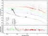 |
Fig. 4 Fit to the light curve in X-ray and optical/NIR Vr′Ri′IJHKS bands including a total of five energy injections. Data before 500 s are excluded from the modelling, as well as the strong X-ray flare. The light curves have been offset by constant factors as given in the figure legend for better legibility. The Bg′ bands are affected by additional Lyman forest absorption and were not included in the fit. For the Bg′ bands, the model predictions have been multiplied by 0.50 and 0.55 respectively to match them with the data. The residuals are clearly improved in comparison to those plotted in Fig. 3, but short-timescale variations like the one at 0.7 days are still not fitted satisfactorily. |
If we take the X-ray data from Dai et al. (2007) and fit it with the parameters of our double smoothly-broken power law fit using X-ray data from 0.06 days onward, we concur that the fit is marginally acceptable, with χ2/d.o.f. = 1.6 for 40 degrees of freedom. Using our own X-ray reduction, we obtain a worse result, with χ2/d.o.f. = 1.7 for 22 degrees of freedom. Similarly, with X-ray data from the Swift XRT repository (Evans et al. 2007, 2009), the fit is rejected (χ2/d.o.f. = 2.3 for 33 degrees of freedom). The reason is that there are less data points, but with smaller error bars, so the outliers are weighted more strongly. A fit to the X-ray data alone results in a much earlier break time and slopes that are less steep (again in agreement with Dai et al. 2007), but we caution that the late X-ray afterglow is only sparsely sampled and shows large scatter. For the three different reductions, we derive the following values using a smoothly-broken power law (a double-broken power law yields no statistical improvement), with n = 10 fixed and no host galaxy: α1 = 0.92 ± 0.05, α2 = 3.02 ± 0.63, tb = 1.38 ± 0.25 (XRT repository light curve); α1 = 0.90 ± 0.05, α2 = 2.78 ± 0.61, tb = 1.34 ± 0.28 (our XRT reduction); α1 = −0.29 ± 0.56, α2 = 1.69 ± 0.17, tb = 0.16 ± 0.05 (Dai et al. 2007 data). As can be seen, the latter fit is very different from the other two (which agree fully within error bars). Even using data from 0.01 days onward (end of the X-ray flare), the fit is still significantly different: α1 = 0.43 ± 0.06, α2 = 1.69 ± 0.17, tb = 0.25 ± 0.06.
4.2. Modelling the light curve with energy injections
Motivated by the similarities to such highly variable light curves as that of the afterglow of GRB 021004, which was successfully modelled by multiple energy injections (“refreshed shocks”) (de Ugarte Postigo et al. 2005), we used the code of Jóhannesson et al. (2006) to model the afterglow light curve. The code numerically solves the kinematic equations of an expanding shock front and calculates the resulting synchrotron emission. Relativistic effects are fully taken into account and the code supports delayed energy injection episodes. Several energy injection episodes are applied as a possible scenario to explain the rebrightenings and shallow decay of the afterglow. Preliminary results on a smaller data set were presented in Jóhannesson et al. (2009). The number and a time range for the energy injections have to be inserted as initial guess for the fit and the fit then adjusts them to the best possible time within that range and determines the magnitude of the injection. As the very early data likely contain some signature of the prompt emission, we exclude all data before 400 s as well as the very bright X-ray flare. Due to Lyman forest blanketing, data in B and g′ bands were excluded from the fit. The V band is also affected by the blanketing, but was corrected with the model from Madau (1995) (brightened by 0.17 mag) and included in the fit to have a better spectral coverage at early times.
Figure 4 shows the best fit
(χ2/d.o.f. = 2.0) found using a model with a total of five
energy injections: at 0.01, 0.04, 0.07, 0.35 and 0.60 days. Each energy injection episode
adds 2 free parametres to the fit in addition to the 6 parametres needed for the standard
afterglow model discussed below. The initial energy injected into the outflow is3 erg. The
energy injections then add 1.8, 4.1, 4.2, 8, and finally 14 times the initial energy
release E0 to the afterglow, for a total energy release in the
afterglow of
erg. The
energy injections then add 1.8, 4.1, 4.2, 8, and finally 14 times the initial energy
release E0 to the afterglow, for a total energy release in the
afterglow of  erg.
erg.
The first three injections are responsible for the shallow afterglow decay between 0.008 and 0.25 days. The quality of the data does not allow to discriminate between this three-injection scenario and a continuous injection. Using a lower number of injections does not yield a satisfactory fit to the observed data. Since there are no direct indications of injections in the light curve, the time of each of the three injections is not well determined. A direct consequence of this is that the energy of each individual injection in this phase is not well determined, while the total energy released is fairly consistent. The time and energy of the last two injections are, however, better constrained by the data.
Further results of the modelling are a high density of the circumburst medium of
 cm
-3 (a high value, comparable to the high-z GRB 050904, Frail et al. 2006), a rather low opening angle of
cm
-3 (a high value, comparable to the high-z GRB 050904, Frail et al. 2006), a rather low opening angle of
 and an
electron index of
and an
electron index of  (host galaxy
extinction is assumed to be negligible, see Sect. 4.3). The peak frequency νm passes through the
optical/NIR at very early times, while the data are most likely affected by the prompt
emission. The cooling break νc is between the optical and
X-rays up to 6 days after the burst, i.e., over the whole data span. Furthermore, we find
(host galaxy
extinction is assumed to be negligible, see Sect. 4.3). The peak frequency νm passes through the
optical/NIR at very early times, while the data are most likely affected by the prompt
emission. The cooling break νc is between the optical and
X-rays up to 6 days after the burst, i.e., over the whole data span. Furthermore, we find
 and
and
 , with
εe being the fraction of the energy in the electron
population and εB the fraction of the energy
in the magnetic field. Note that the definition of εe has been
changed in the model from Jóhannesson et al. (2006)
to the definition of Panaitescu & Kumar
(2001) to allow for p < 2 in the model.
This model reproduces the global properties of the optical/NIR light curves well, with the
rather high χ2/d.o.f. = 2.0 resulting from rapid variability
in the late time afterglow. This is incompatible with the homogeneous shock front assumed
in the numerical code. The X-ray light curve is also fitted reasonably well.
, with
εe being the fraction of the energy in the electron
population and εB the fraction of the energy
in the magnetic field. Note that the definition of εe has been
changed in the model from Jóhannesson et al. (2006)
to the definition of Panaitescu & Kumar
(2001) to allow for p < 2 in the model.
This model reproduces the global properties of the optical/NIR light curves well, with the
rather high χ2/d.o.f. = 2.0 resulting from rapid variability
in the late time afterglow. This is incompatible with the homogeneous shock front assumed
in the numerical code. The X-ray light curve is also fitted reasonably well.
4.3. The spectral energy distribution and host extinction
Following the procedures outlined in Kann et al. (2006), we derive the optical spectral energy distribution (SED) of the GRB 060526 afterglow and fit it with several dust models (Milky Way, MW; Large Magellanic Cloud, LMC; and Small Magellanic Cloud, SMC; Pei 1992) to derive the line-of-sight extinction in the host galaxy. Due to the strongly variable light curve, we choose the approach Kann et al. (2006) used for the SED of GRB 030329, and shift the other bands to the RC-band zero point to derive the colours. With this method, we can also look for colour changes. There may be marginal variations in B−R, but this colour remains constant within conservative errors, and is more sensitive to Lyman forest blanketing, as different filters will suffer a different amount of blanketing.
The SED clearly shows the decreasing flux in the B, g′ and V bands, and especially in the uvw2uvm2uvw1u bands, where only upper limits are found, due to the Lyman forest blanketing as well as the Lyman cutoff (see Fig. 5), and we thus do not include these filters in our fit. Given the size of the errors, all fits, even with no extinction, are acceptable (see Table 4) and we are thus unable to prefer one dust model over another. The lack of z band data does not allow us to constrain the existence of a 2175 Å bump, therefore we have no evidence in favor of or ruling out MW and LMC dust. We do note, though, that MW dust leads to slightly negative extinction, while the LMC dust fit yields large errors. Thus, we henceforth use the SMC dust fit, as this is the most common dust type found in GRB host galaxies, both in pre-Swift (Kann et al. 2006; Starling et al. 2007) and Swift-era (Schady et al. 2007; Kann et al. 2010) results. Note that for SMC dust, the extinction is 0 within errors as well.
Assuming the cooling break νc to lie
blueward of the optical bands (highly likely considering the X-ray spectral slope
βX ≈ 1, Dai
et al. 2007,and the result of the numerical modelling), the standard fireball
model gives for the electron power law index
p = 2β + 1 = 2.10 ± 0.40. This result (albeit with large
errors) is in agreement with the result from the broadband modelling (Sect. 4.2) and with the canonical p = 2.2, and
very similar to many other GRB afterglows (e.g. Kann
et al. 2006; Starling et al. 2007). Our
results are in contrast to Dai et al. (2007), who
derive a very steep slope  from
Br′i′ data only
(correcting for Lyman absorption) and conclude that the optical and the X-ray data lie on
the same slope.
from
Br′i′ data only
(correcting for Lyman absorption) and conclude that the optical and the X-ray data lie on
the same slope.
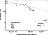 |
Fig. 5 Spectral energy distribution of the afterglow of GRB 060526 in uvw2uvm2uvw1uBg′Vr′RCi′ICJHKS, and fits with no extinction (straight black line), MW extinction (dotted line), LMC extinction (dashed line) and SMC extinction (thick dash-dotted line). The fit with MW dust finds (unphysical) negative extinction, causing an “emissive component” instead of a 2175 Å absorption bump. Data beyond 2.2 × 10¹⁵ Hz (Vg′Buuvw1uvm2uvw2) were not included in the fit due to Lyman forest blanketing, the grey curves represent extrapolations. The extinction curves of Pei (1992) are not correctly defined beyond 3.2 × 10¹⁵ Hz. The UVOT UV filters are upper limits only, showing the strong flux decrease beyond the Lyman cutoff. The flux density scale is measured at the break time. |
Fits to the spectral energy distribution of GRB 060526.
4.4. Host search
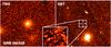 |
Fig. 6 Left panel: an image from the TNG with the afterglow present. Right panel: the same region observed with HST/ACS and a zoom-in around the region of the afterglow. There is no source detected at the afterglow position itself down to a limit of F775W(AB) > 28.5. The brighter spot to the South-East in the zoomed HST image corresponds to the host candidate from the VLT mentioned in the text. A color version of the figure is available in the online version of the article. |
In the late-time VLT images, we do not detect any source at the position of the afterglow down to a limit of RC > 27.1 mag (which transforms into an absolute magnitude limit of MR > − 20.1). There is one source present at ~1″̣5 South-East of the afterglow position with RC = 26.4 ± 0.2, which at a redshift of z = 3.221 would transform into a physical offset between GRB and host galaxy of ~11.5 kpc. A long-slit spectrum covering the afterglow position and this galaxy does not show any trace at these positions. If this galaxy was associated with the GRB, it would be one of the largest offsets between a long-duration GRB and its host galaxy known (Bloom et al. 2002). The strong absorption lines from the ISM seen in the afterglow spectrum (see Sect. 5) as well as the high circumburst density inferred from the numerical modeling (see Sect. 4.2) do in fact not favour a large distance from the host galaxy. A position outside of their host galaxies had been inferred for GRB 070125 (Cenko et al. 2008) and GRB 071003 (Perley et al. 2008b), however, those spectra showed very weak absorption lines, contrary to what we observe for GRB 060526. Concluding, we have no direct spectroscopic evidence for or against an association of the GRB with the galaxy.
We also observed the field with ACS on HST. Astrometry was performed relative to our TNG image, yielding a position accurate to ~0.1″. At the location of the burst we do not find any evidence for an underlying host galaxy. To estimate the limits we place 50 apertures randomly on the sky and measure the standard deviation in their count rates. This implies that the underlying host galaxy of GRB 060526 is fainter than F775W(AB) >28.5 (3σ) or an absolute magnitude of M(1500 Å) > –18.3 mag which is fainter than 0.5 L* according to Gabasch et al. (2004). The flux density at the host position is 0.004 ± 0.005 μJy.
Host galaxies of long-duration GRBs have often been found to be faint irregular galaxies (Fruchter et al. 2006; Christensen et al. 2004) which are difficult to detect at higher redshifts. So far, there are only eight bursts with z > 3 where the detection of a host galaxy has been published, namely GRB 971214 (z = 3.418, Kulkarni et al. 1998), GRB 000131 (z = 4.500, Andersen et al. 2000; Fruchter et al. 2006), GRB 030323 (z = 3.3718, Vreeswijk et al. 2004), GRB 060206 (z = 4.04795, Fynbo et al. 2006; Thöne et al. 2008; Chen at al. 2009), GRB 060210 (z = 3.9133, Fynbo et al. 2009; Perley et al. 2009), GRB 060605 (z = 3.773, Ferrero et al. 2009), GRB 090205 (z = 4.6503, D’Avanzo et al. 2010), and GRB 090323 (z = 3.568, Cenko et al. 2010; McBreen et al. 2010). The host galaxies of GRB 020124 (Berger et al. 2002; Chen at al. 2009), GRB 050730, GRB 050908, GRB 060607A, GRB 070721B (all Chen at al. 2009), GRB 050904 (Berger et al. 2007) and GRB 060510B (Perley et al. 2009), on the other hand, were not detected to very deep limits in the optical and the NIR.
The distribution of pre-Swift RC band host galaxy magnitudes peaks at RC(AB) = 25 (Fruchter et al. 2006) but extends out to 29 with a typical redshift z ≈ 1.4. Swift GRBs (and thus their hosts) however have a higher mean redshift of z = 2.8 (Jakobsson et al. 2006a)4, so the distribution will be shifted out to even fainter magnitudes. Ovaldsen et al. (2007) also find a higher magnitude for Swift hosts than for pre-Swift bursts by comparing the expected detection rate from pre-Swift hosts with detections and upper limits derived from imaging the fields of 24 Swift and HETE II bursts from 2005–2006.
5. Spectroscopy results
5.1. Line identification
We detect a range of metal absorption lines as well as a Lyman limit system (LLS) originating in the host galaxy of GRB 060526. A redshift of z = 3.221 was determined in Jakobsson et al. (2006b) from a number of these absorption lines using the spectra taken with the 600V grism presented in this article.
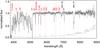 |
Fig. 7 The spectrum taken with 300V grism, the two exposures have been combined to improve the S/N. The identified lines as well as the main atmospheric absorption bands are labelled. The line at the bottom shows the error spectrum. A color version of the figure is available in the online version of the article. |
Most of the lines were fitted from the combined 600V spectrum which covers all metal absorption lines detected longwards of Ly-α, but provides a higher resolution than the 300V spectra. The 600I spectra only covers the AlII λ 1670 line at the same resolution as the 600V grism. The range of 1200B is entirely within the Lyman-α forest but does not have a high enough resolution to deblend metal transitions from absorption caused by the Ly-α forest lines. We do, however, detect Ly-β and Ly-γ absorption in the 1200B grism. In the blue end of the 300V spectrum, one can clearly see the 915 Å Lyman break at the redshift of the host galaxy. In Fig. 7, we show the combined spectrum of the 300V grism with the identified lines indicated. We note that we do not detect any intervening system in the sightline towards GRB 060526, which is rather unusual for a GRB sightline, in particular at that redshift (see, e.g., Prochter et al. 2006). Taking the strong Mg ii λ 2796, 2803 doublet, the redshift path probed for any intervening system is between z ~ 0.8 and 2.2. The 3σ limits on the non-detection of the Mg ii doublet vary between 0.17 Å (z = 0.8) and 0.82 Å (z = 2.2) (rest frame).
In order to determine the equivalent width (EW) of the strong absorption lines, we fitted the continuum around the lines in regions that were free of absorption and summed over the absorption contained within two times the full-width at half-maximum (FWHM) of the lines. For weak lines, we obtained better results due to the low S/N by fitting Gaussians. For this fit, we used a modified version of the gaussfit procedure provided in IDL5 which is more reliable in determining the continuum and fitting the actual line even if it is slightly blended with a neighbouring line. The upper limits on the EWs for a range of ions noted in Table 5 was determined from the spectra taken with the 300V grism due to the better S/N of those spectra. Between the individual spectra, we do not find any variability in the EW of the individual absorption lines.
S ii λ 1259, Si ii λ 1260 and Fe ii λ 1260 are blended and cannot be fitted separately. We therefore cannot consider them for the derivation of the column density from the curve of growth fit as described below and only give the total EW in Table 5. In contrast to what is noted in Jakobsson et al. (2006b), we cannot reliably detect any fine-structure lines and only give an upper limit for Si ii*. Fine-structure lines would be a clear indication that the detected absorption lines indeed originate in the host galaxy of the GRB, as they are assumed to be produced by UV pumping from the afterglow (e.g. Prochaska et al. 2006; Vreeswijk et al. 2007; D’Elia et al. 2009). The redshift derived is therefore to be strictly taken as a lower limit only, the detection of the Lyman α forest redward of the proposed redshift, however, excludes a significantly higher redshift for the burst.
EWs of detected absorption lines and 2σ upper limits on some undetected lines, the EW for the blended systems include the contributions from all lines.
5.2. Column densities from curve of growth analysis
Some of the strong absorption lines are saturated, which is a problem in low resolution spectra as the damping wings are not resolved and Voigt profile (VP) fitting cannot be adopted to derive a reliable column density. Furthermore, high resolution spectra of GRBs (Prochaska 2006) have shown that the strong metal absorption lines unresolved in low resolution spectra usually consist of a number of narrow, unsaturated components that would allow an accurate determination of the column density by fitting the different components separately.
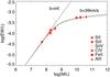 |
Fig. 8 Multi-ion single-component curve of growth fit for the absorption systems in GRB 060526 using 6 different ions. The CoG is expressed in units of the column density “N”, the oscillator strength of the transition “f” and the wavelength of the transition. As comparison, b = ∞ is plotted, the dotted line marks the 1 σ deviation from the fit. A color version of the figure is available in the online version of the article. |
If only low resolution spectra are available, one has to adopt a curve of growth (CoG) analysis (Spitzer 1978; Savage & Sembach 1996) which directly relates the EW to the column density on the linear part of the CoG where the lines are not saturated (optical depth τ0 < 1), but depends on the Doppler b parameter of the medium on the flat part of the curve which applies for mildly saturated lines. For GRBs, one usually has to do a multiple-ion single-component CoG (MISC-CoG) analysis, adopting the same effective Doppler parameter for all ions. Here, we used all unblended ionic lines that were not heavily saturated, namely S ii, Si ii, Fe ii, Al ii as well as C iv and Si iv and calculate the χ2 minimum going through the parameter space for the column densities of each ion and a range of b parameters. We then find the best fit for b = 39 ± 3 km s-1 (see Fig. 8) and the column densities as noted in Table 5. Most of the ions lie near the linear part of the CoG and are therefore rather independent of b, Si ii and Al ii lie on the flat part of the CoG and the column densities are only noted as lower limits as derived from the linear part of the CoG. We excluded the saturated O i and C ii transitions from the fit and only list lower limits for these two ions for which we take the column density resulting from the linear part of the CoG. We also discarded the blended absorption lines of Si ii λ 1260, S ii and Fe ii even though Si ii is the dominant contribution to the absorption since we detect two other unblended Si ii transitions at λ 1304 and λ 1526 Å.
There are several problems connected with the use of the CoG that have to be considered. Different ionisation levels should actually be treated in separate analyses as they might occur in different regions in the absorbing system. However, we assume that the absorption takes place in a relatively small region of the host galaxy and the resolution of the spectrum does resolve different components of the absorbing material in the host galaxy. Therefore, we also fit the higher ionisation levels of Si iv and C iv in the same CoG. Furthermore, they lie close to the linear part of the CoG and excluding them from the common fit would not change the derived b parameter very much. Another problem with doing multiple-ion CoG analysis using strong lines in low-resolution spectra has been noted by Prochaska (2006), who compared column densities derived from low resolution spectra and CoG with high resolution data and VP fitting from the same bursts. He found that when including saturated lines in the fit, column densities are generally underestimated. Indications for that are if an effective b parameter of ≫ 20 km s-1 is found, since strong lines actually consist of a range of components with b < 20 km s-1. Savaglio (2006) however performed a similar analysis using CoG and the apparent optical depth (AOD) method as described in Pettini et al. (2002), which can be applied for medium resolution high S/N spectra, and found a good agreement between the two methods. The column densities of the saturated lines Al ii and Si ii are infact rather sensitive to the adopted b parameter. These lines very likely consist of a number of unresolved weaker components which would lie on the linear part of the CoG, the real errors should therefore be larger but are difficult to estimate.
5.3. Metallicity and relative abundances
Absorption lines that are likely not affected by dust depletion can be used to derive a metallicity of the medium in the line of sight to the GRB. The least dust-depleted element is Zn, which is, however, undetected in our spectra. We then use the relatively weak lines S ii and Fe ii derive relative metallicities compared to the hydrogen density with [M/H] = log (NM/NH) − log (NM/NH)⊙ using solar abundances from Asplund et al. (2005). Here we derive metallicities of [S/H] = −0.57 ± 0.25 and [Fe/H] = −1.22 ± 0.24.
Fe is usually affected by dust depletion (Savage & Sembach 1996) and corrections have to be adopted. Using the relation between the Zn and Fe abundance in Savaglio (2006), we find a metallicity of [Fe/H] = −1.09 ± 0.24 which marginally agrees within the errors with the value derived from sulphur. The only detected and unblended S ii line at λ 1253, however, is only marginally detected and therefore the EW has large errors. The Fe ii doublet taken for the CoG fit, in contrast, is also slightly blended, but the fit of the stronger component can be considered as reliable. Despite the dust depletion, the metallicity derived from Fe might be the most reliable one in this case and we therefore assume a metallicity of [Fe/H] = –1.09 for the host of GRB 060526.
Independent of the ion used, the metallicity is rather high compared to other galaxies at redshift z ≈ 3, but among the typical metallicities derived for other GRB hosts (Fynbo et al. 2006) at that redshift. For those measurements, different ions have been used depending on the quality and the wavelength coverage of the spectra. Our results show that caution is required when comparing the metallicities derived from different elements, as they might be differently affected by dust depletion and/or evolution. This is especially true when saturated lines in low resolution spectra are used to derive the column densities and hence the abundances as it is the case for, e.g., GRB 000926 (Savaglio et al. 2003) and GRB 011211 (Vreeswijk et al. 2006). For GRB 050401 (Watson et al. 2006) and GRB 050505 (Berger et al. 2006), the authors themselves note that due to saturation the reported metallicity is indeed a lower limit.
Our spectra do not allow us to determine a dust depletion pattern from the relative abundances of heavier elements, since at least four elements out of Zn, Si, Mn, Cr, Fe, Ni or S are necessary to do such a fit. The difference in the relative abundances between S and Fe might suggest the presence of some dust in the line-of-sight towards the GRB, however, large extinction is excluded from the afterglow SED. On the other hand, this difference could also be due to an enhancement in α element production6 which is likely to happen in the young star-forming host of a GRB. Generally, GRB hosts have higher α/Fe ratios than QSO-DLAs (Prochaska et al. 2007), which can either be interpreted as large dust depletion consistent with the higher metallicities of GRB sightlines or as α element enhancement. There are indications that most of the α/Fe ratio is due to dust depletion traced by a large [Zn/Fe] or [Ti/Fe] < 0. The latter is assumed to be a clear indicator of dust depletion ([Ti/Fe] < 0) vs. α enhancement ([Ti/Fe] > 0) (Dessauges-Zavadsky et al. 2002). Both elements are, however, not detected and the limit on Zn does not lead to a strong constraint on the [Zn/Fe] ratio to settle this issue in the case of GRB 060526.
The ratio between high and low ionisation species in the spectrum clearly shows that most of the material in the line of sight is in a low ionization state. Si iv and C iv have rather low column densities and lie close to the linear part of the CoG in contrast to their low ionization species Si ii and C ii which are both saturated, whereas Al iii is not even detected in our spectra. We then derive column density ratios of log(Si iv/Si ii) = −2.37, log(C iv/C ii) < −1.45 and log(Al iii/Al ii) < −2.41. From the large sample of Swift long GRB afterglow spectra (Fynbo et al. 2009), this seems fairly normal for an average GRB sightline. However, the few GRBs occurring in LLSs (log NHI/cm-2 < 20.3) usually show a higher fraction of ionized material compared to GRB-DLA sightlines. This might either be due to decreased shielding of the highly ionizing afterglow flux by the lower hydrogen column density, by a rather special arrangement of the GRB inside the host galaxy or simply by a small host galaxy. Since our spectra show a low fraction of highly ionized material this implies that the absorbing material has a relatively large distance from the GRB.
We do not detect N v in our spectra but provide an upper limit of log N < 13.66. N v was detected in only four sightlines towards GRBs (Prochaska et al. 2008) and likely traces the immediate environment of the GRB as it has a high ionization potential and requires a strong radiation field. Our upper limit is lower than the column densities for those GRB sightlines where N v could be detected which again implies that the absorbing gas probed by our spectra are most likely not close to the GRB itself. Furthermore, we do not detect any fine structure lines and only derive an upper limit on Si ii* of log N/cm-2 < 12.76. Fine structure lines are assumed to be pumped by the UV radiation field of the GRB (Vreeswijk et al. 2007) which also indicates that the gas is likely very far from the GRB itself. Si ii* requires a less strong radiation field and has been detected in Lyman break galaxies (Pettini et al. 2002) where the UV radiation from young stars provides the necessary radiation field.
6. Discussion and conclusions
GRB 060526 had a relatively bright afterglow that allowed us to obtain a solid dataset, both photometrically and spectroscopically. We achieved a dense light curve coverage over several days which allowed a detailed study of the afterglow properties, and obtained a series of low resolution but high signal-to-noise spectra to study the host environment.
The optical light curve can be fitted with a double smoothly-broken power law with breaks at tb1 = 0.090 ± 0.005 and tb = 2.216 ± 0.049 days, and decay slopes of αplateau = 0.288 ± 0.026, α1 = 0.971 ± 0.008, and α2 = 2.524 ± 0.052. The dense sampling of especially the RC-band light curve reveals additional variability on top of the power laws. These features could be explained either by extended activity of the central engine or through interactions of the shock with the interstellar medium. For the case that the variability arises from external shocks, several mechanisms have been considered. In GRB 021004, both density variations of the external medium into which the GRB jet plows and angular inhomogenities of the jet surface were considered (Nakar et al. 2003). However, Nakar & Granot (2007) show that density variations would cause much smaller fluctuations than those observed in GRB afterglows and can therefore be ruled out. Another possibility is the injection of additional energy into the shock by slower shells that catch up with the shocked region as it decelerates, this model was used successfully to describe GRB 021004 (de Ugarte Postigo et al. 2005) and also works better than two other models (double jet and density fluctuations) to describe the highly complex light curve of GRB 030329 (Huang et al. 2006). Thus, variability can give either information on the medium surrounding the GRB or on the activity of the central engine. A more intriguing possibility is that the flares may be emitted from another region closer to the central engine, resulting from late internal shocks. Powerful X-ray flares that are attributed to late central engine activity have been observed in about 50% of all Swift GRBs (e.g. Burrows et al. 2005; Chincarini at al. 2007; Krimm et al. 2007), and strong optical/NIR flaring contemporaneous with the GRB prompt emission may also occur (Vestrand et al. 2005, 2006; Blake et al. 2005; Racusin et al. 2008), thus making optical flares from late central engine activity an interesting prospect (Kann 2007; Malesani et al. 2007).
Indeed, Dai et al. (2007) have suggested that the optical variability of the afterglow of GRB 060526 is due to flares from late internal shocks (the very early rapid optical variability we present here is very probably due to central engine activity, as it is seen contemporaneously in gamma and X-rays). Khamitov et al. (2007), on the other hand, conclude that the short timescale of the variabilities requires the jet to be non-relativistic already at ~1 day and could then be explained by external density fluctuations. Our analysis lends tentative support to the notion of flares from internal shocks, finding decay slopes for two flares that exceed what should be possible from external shocks. But we caution that the errors of these fits are large due to a low amount of data in the decaying parts. Furthermore, globally, a model using refreshed external shocks is able to account for the light curve variations, although microvariability remains. This creates the intriguing possibility of reverberation effects (see Vestrand et al. 2006, for a case of reverberation between gamma-rays and optical emission). Short flares in the X-ray or optical bands signal internal shocks from long-term central engine activity, and when these shells catch up with the forward shock front, they re-energise the external forward shock. The detection of such behaviour would probably require dense multi-band observations of a bright afterglow to search for SED changes at high time resolution combined with detailed modelling of the data. This way, one could discern between internal shocks (which are expected to have a different spectral index from the forward shock afterglow) and refreshed, external shocks (which are achromatic). Our data set of the afterglow of GRB 060526 does not allow us such a detailed decomposition.
From the analysis of our low resolution spectra with different resolutions, we detect a LLS and a number of metal absorption lines that all lie at a redshift of z = 3.221. The low resolution only allows us to derive column densities from measuring the EWs of the absorption lines and adopt a MISC-CoG analysis where we exclude the most saturated as well as blended transitions. We find a best fit for the Doppler parameter of b = 39 ± 3 km s-1 and most of the ions used for the fit lie on the linear part of the CoG which allows a relatively reliable determination of the column densities. The relative abundances of different metals in the spectra indicate some dust extinction, but an intrinsic difference due to enhancement of the production of certain elements cannot be excluded. The very low amount of dust detected in the afterglow SED may indicate that the latter might be the favored possibility.
The column density of neutral hydrogen is rather low compared to other GRBs. We derive a metallicity for the host of [Fe/H] = −1.09 which is slightly higher than metallicities determined from other GRB afterglow spectra. According to the definition of QSO absorbers, the host of GRB 060526 is classified as a LLS (19 < log NHI/cm-2 < 20.3), which seem to have on average higher metallicities than damped Lyman α systems (DLA; Peroux et al. 2007) and a steeper evolution towards lower redshifts. Around redshift 3, however, the metallicities of both samples are within the same range. Also, GRB hosts show a trend towards increasing metallicity with lower redshifts (Fynbo et al. 2006; Savaglio 2006). Taking into account that most of the sample used only low-resolution spectra to derive the metallicity (which only gives lower limits for the column densities and the metallicity) this evolution might, however, not be as pronounced as for DLAs and LLS. This might imply that the enrichment of the ISM in the early universe had taken place at earlier times than assumed. The absorbing material along the line-of-sight is mostly in the neutral state, as usually observed for long GRB-DLAs, while sightlines with lower log NHI often contain more ionized material. This might either imply that we have a very small host galaxy or that the GRB is placed somewhere in the outskirts of its host. In general, the low ionization points to a relatively large distance of the absorbing material from the GRB itself.
There is no underlying host galaxy of GRB 060526 detected down to a deep limit of 28.5 mag (in F775W AB) in HST/ACS data. At that redshift, this means the host has an absolute magnitude M(1500 Å) > −18.3 mag, fainter than an 0.5 L* galaxy at that redshift. Long GRBs have been found to occur in actively star-forming galaxies and star formation is assumed to shift towards smaller and fainter galaxies over time (e.g. Cowie et al. 1996) while massive galaxies prove to be rather unchanged throughout the history of the universe (e.g. Abraham et al. 1999; Heavens et al. 2004). One would therefore expect that GRB hosts should also have higher luminosities towards higher redshifts. Fynbo et al. (2008) concluded that the observed metallicity distribution of GRB hosts (as well as QSO absorbers) at z ≈ 3 can be explained by the luminosity function of galaxies at that redshift and assuming a luminosity-metallicity relation as derived for other high-redshift samples (Ledoux et al. 2006; Erb et al. 2006). The non-detection of the host of GRB 060526 down to deep limits, however, would not support this suggested evolution. The data neither strongly support nor allow us to rule out that the GRB is associated with a nearby galaxy at ~11.5 kpc. While the offset would be very large compared to typical long GRB offsets, it is possible the burst occurred in a locally dense star-forming region which is not detected even in our very deep imaging.
Online material
Broad band observations of GRB 060526, times given are the midpoint of the observations.
Notes. Data have not been corrected for Galactic extinction. All data except the Keck/LRIS g′ and the HST F775W data points (in AB magnitudes) are in Vega magnitudes. UVOT is the 30 cm UltraViolet and Optical Telescope onboard the Swift satellite.
Maidanak is the 1.5 m telescope of the Maidanak observatory in Uzbekistan.
RTT150 is the 1.5 m Russian-Turkish Telescope at TÜBİTAK National Observatory on Mount Bakyrlytepe, Antalya, Turkey.
MOSCA is the MOSaic CAmera on the 2.5 m Nordic Optical Telescope, La Palma, Canary Islands, Spain.
Keck/LRIS is the Low Resolution Imaging Spectrograph on the 10 m Keck I telescope, Mauna Kea, Hawaii, USA.
DOLORES is the Device Optimized for the LOw RESolution detector on the 3.6 m TNG (Telescopio Nazionale Galileo) telescope on La Palma, Canary Islands, Spain.
MIRO is the 1.2 m telescope of the Mt. Abu Infrared Observatory, India.
BFOSC is the Bologna Faint Object Spectrograph & Camera at the G. D. Cassini 152 cm telescope of the Bologna University, Loiano, Italy.
DFOSC is the Danish Faint Object Spectrograph and Camera on the Danish 1.54 m telescope on La Silla, Chile.
Watcher is the 0.3 m Watcher robotic telescope at Boyden Observatory, South Africa.
Shajn is the 2.6 m Shajn telescope of the Crimean Astrophysical Observatory (CrAO), Ukraine.
TLS 1.34 m is the 1.34 m Schmidt telescope of the Thüringer Landessternwarte Tautenburg, Germany.
ALFOSC is the Andalucia Faint Object Spectrograph and Camera on the 2.5 m Nordic Optical Telescope, La Palma, Canary Islands, Spain.
FORS2 is the FOcal Reducer and low dispersion Spectrograph 2 on the 8.2 m Very Large Telescope, Paranal Observatory, Chile.
ROTSE is the 0.3 m Robotic Optical Transient Search Experiment III-B telescope at the HESS site, Mt. Gamsberg, Namibia.
ANDICAM is the A Novel Double-Imaging CAMera detector on the 1.3 m Small and Moderate Aperture Research Telescope System (SMARTS) telescope at the Cerro Tololo Interamerican Observatory in Chile.
PAIRITEL is the 1.3 m Peters Automatic InfraRed Imaging TELescope on Mt. Hopkins, Arizona, USA.
HST ACS is the Hubble Space Telescope equipped with the Advanced Camera for Surveys.
Note, though, that Dai et al. (2008) argue that optical follow-up in the Swift era, especially with UVOT only, often does not persist long enough (and to enough depth) to find jet breaks.
The error limits presented here are 1σ estimates, but due to degeneracy in the model parameters, the actual range of parameter values can be much larger.
An updated version of the redshift distribution can be found under http://raunvis.hi.is/~pja/GRBsample.html – as of July 1, 2010, the mean redshift has become lower, z = 2.19, see also Fynbo et al. (2009), who find a mean and median of z = 2.2.
Available at http://www.pa.iasf.cnr.it/~nicastro/IDL/Lib/gfit.pro
α elements are produced in massive, metal-poor stars through the α process and include elements with integer multiples of the He nucleus mass such as O, Si, S, Ca, Mg and Ti.
Acknowledgments
We thank the referees for constructive comments that improved the paper. C.C.T. wants to thank Cédric Ledoux for comments on the curve-of-growth analysis and S. Campana for comments on the text. We thank the support astronomer and staff at the Nordic Optical Telescope for obtaining the observations.
The Dark Cosmology Centre is funded by the DNRF. H.D. acknowledges support from the Research Council of Norway. L.H. acknowledges support from Science Foundation Ireland grant 07/RFP/PHYF295. P.J. acknowledges support by a Marie Curie European Reintegration Grant within the 7th European Community Framework Program and a Grant of Excellence from the Icelandic Research Fund. I.F.B. acknowledges partial support by the RFFI grant “09-02-97013-povolzhe”. P.A.C. gratefully acknowledges the support of NWO under grant 639.043.302. C.B., A.G., and G.G. acknowledge the University of Bologna for the funds Progetti di Ricerca Pluriennali. S.F. acknowledges the support of the Irish Research Council for Science, Engineering and Technology, cofunded by Marie Curie Actions under FP7.
Based on observations made with the Nordic Optical Telescope, operated on the island of La Palma jointly by Denmark, Finland, Iceland, Norway, and Sweden, with the William Herschel Telescope and the Telescopio Nazionale Galileo in the Spanish Observatorio del Roque de los Muchachos of the Instituto de Astrofísica de Canarias and at the Astronomical Observatory of Bologna in Loiano (Italy). Collection of SMARTS data is supported by NSF-AST 0707627. MIRO is supported by the Department of Space, Govt. of India. The Peters Automated Infrared Imaging Telescope (PAIRITEL) is operated by the Smithsonian Astrophysical Observatory (SAO) and was made possible by a grant from the Harvard University Milton Fund, the camera loan from the University of Virginia, and the continued support of the SAO and UC Berkeley. The PAIRITEL project and JSB are further supported by NASA/Swift Guest Investigator Grant NNG06GH50G. We thank M. Skrutskie for his continued support of the PAIRITEL project. The W.M. Keck Observatory is operated as a scientific partnership among the California Institute of Technology, the University of California and the National Aeronautics and Space Administration and was made possible by the generous financial support of the W.M. Keck Foundation. I.F.B., R.A.B., I.M.Kh., M.N.P., R.A.S. extend thanks to TÜBİTAK, IKI, and KSU for a partial supports in using the RTT150 (Russian-Turkish 1.5-m telescope in Antalya).
References
- Abraham, R. G., Ellis, R. S., Fabian, A. C., Tanvir, N. R., & Glazebrook, K. 1999, MNRAS, 303, 641 [NASA ADS] [CrossRef] [Google Scholar]
- Akerlof, C., Balsano, R., Barthelmy, S., et al. 1999, Nature, 398, 400 [NASA ADS] [CrossRef] [Google Scholar]
- Andersen, M. I., Hjorth, J., Pedersen, H., et al. 2000, A&A, 364, L54 [NASA ADS] [Google Scholar]
- Antonelli, L. A., Testa, V., Romano, P., et al. 2006, A&A, 456, 509 [NASA ADS] [CrossRef] [EDP Sciences] [Google Scholar]
- Arnaud, K. A. 1996, Astronomical Data Analysis Software and Systems V, 101, 17 [NASA ADS] [Google Scholar]
- Asplund, M., Grevesse, N., & Sauval, A. J. 2005, Cosmic Abundances as Records of Stellar Evolution and Nucleosynthesis in honor of David L. Lambert, ed. G. Thomas, III Barnes, N. Frank Bash, ASP Conf. Ser., 336, Proc. Symp. held 17–19 June, 2004 in Austin, Texas. 25 (San Francisco: ASP) [Google Scholar]
- Berger, E., & Gladders, M. 2006, GCN 5170 [Google Scholar]
- Berger, E., Kulkarni, S. R., Bloom, J. S., et al. 2002, ApJ, 581, 981 [NASA ADS] [CrossRef] [Google Scholar]
- Berger, E., Penprase, B. E., Cenko, S. B., et al. 2006, ApJ, 462, 979 [NASA ADS] [CrossRef] [Google Scholar]
- Berger, E., Chary, R., Cowie, L. L., et al. 2007, ApJ, 665, 102 [NASA ADS] [CrossRef] [Google Scholar]
- Beuermann, K., Hessman, F. V., Reinsch, K., et al. 1999, A&A, 352, L26 [NASA ADS] [Google Scholar]
- Blake, C. H., Bloom, J. S., Starr, D. L., et al. 2005, Nature, 435, 181 [NASA ADS] [CrossRef] [PubMed] [Google Scholar]
- Bloom, J. S., Kulkarni, S. R., & Djorgovski, S. G. 2002, AJ, 123, 1111 [NASA ADS] [CrossRef] [Google Scholar]
- Brown, P. J., Campana, S., Boyd, P. T., & Marshall, F. E. 2006, GCN 5172 [Google Scholar]
- Burrows, D. N., Romano, P., Falcone, A., et al. 2005, Science, 309, 1833 [NASA ADS] [CrossRef] [PubMed] [Google Scholar]
- Campana, S., Barthelmy, S. D., Boyd, P. T., et al. 2006a, GCN 5162 [Google Scholar]
- Campana, S., Barthelmy, S. D., Burrows, D. N., et al. 2006b, GCN 5163 [Google Scholar]
- Campana, S., Moretti, A., Guidorzi, C., Chincarini, G., & Burrows, D. N. 2006c, GCN 5168 [Google Scholar]
- Campana, S., Thöne, C. C., de Ugarte Postigo, A., et al. 2010, MNRAS, 402, 2429 [NASA ADS] [CrossRef] [Google Scholar]
- Cenko, S. B., Fox, D. B., Penprase, B. E., et al. 2008, ApJ, 677, 441 [NASA ADS] [CrossRef] [Google Scholar]
- Cenko, S. B., Frail, D. A., Harrison, F. A., et al. 2010, ApJ, submitted [arXiv:1004.2900v2] [Google Scholar]
- Chen, H.-W., Perley, D. A., Pollack, L. K., et al. 2009, ApJ, 691, 152 [NASA ADS] [CrossRef] [Google Scholar]
- Chincarini, G., Moretti, A., Romano, P., et al. 2007, ApJ, 671, 1903 [NASA ADS] [CrossRef] [Google Scholar]
- Chornock, R., Perley, D. A., Cenko, S. B., & Bloom, J. S. 2009, GCN 9028 [Google Scholar]
- Christensen, L., Hjorth, J., & Gorosabel, J. 2004, A&A, 425, 913 [NASA ADS] [CrossRef] [EDP Sciences] [Google Scholar]
- Covino, S., D’Avanzo, P., Klotz, A., et al. 2008, MNRAS, 388, 347 [NASA ADS] [CrossRef] [Google Scholar]
- Cowie, L. L., Songaila, A., Hu, E. M., & Cohen, J. G., 1996, AJ, 112, 839 [Google Scholar]
- Dai, Z. G., & Lu, T. 1998, MNRAS, 298, 87 [NASA ADS] [CrossRef] [Google Scholar]
- Dai, X., Halpern, J. P., Morgan, N. D., et al. 2007, ApJ, 658, 509 [NASA ADS] [CrossRef] [Google Scholar]
- Dai, X., Garnavich, P. M., Prieto, J. L., et al. 2008, ApJ, 682, L77 [NASA ADS] [CrossRef] [Google Scholar]
- D’Avanzo, P., Perri, M., Fugazza, D., et al. 2010, A&A, 522, A20 [NASA ADS] [CrossRef] [EDP Sciences] [Google Scholar]
- D’Elia, V., Fiore, F., Perna, R., et al. 2009, ApJ, 694, 332 [NASA ADS] [CrossRef] [Google Scholar]
- Dessauges-Zavadsky, M., Prochaska, J. X., & D’Odoric, S. 2002, A&A, 391, 801 [NASA ADS] [CrossRef] [EDP Sciences] [Google Scholar]
- de Ugarte Postigo, A., Castro-Tirado, A. J., Gorosabel, J., et al. 2005, A&A, 443, 841 [NASA ADS] [CrossRef] [EDP Sciences] [Google Scholar]
- Erb, D. K., Shapley, E. A., & Pettini, M. 2006, ApJ, 644, 813 [NASA ADS] [CrossRef] [Google Scholar]
- Evans, P. A., Beardmore, A. P., Page, K. L., et al. 2007, A&A, 469, 379 [NASA ADS] [CrossRef] [EDP Sciences] [Google Scholar]
- Evans, P. A., Beardmore, A. P., Page, K. L., et al. 2009, MNRAS, 397, 1177 [NASA ADS] [CrossRef] [Google Scholar]
- Fan, Y. Z., Zhang, B., & Wei, D. M. 2005, ApJ, 628, L25 [NASA ADS] [CrossRef] [Google Scholar]
- Ferrero, P., Klose, S., Kann, D. A., et al. 2009, A&A, 497, 729 [NASA ADS] [CrossRef] [EDP Sciences] [Google Scholar]
- Ferrero, A., Hanlon, L., Felletti, R., et al. 2010, Adv. Astron., 2010, 1 [Google Scholar]
- Le Floc’h, E., Duc, P.-A., Mirabel, I. F., et al. 2003, A&A, 400, 499 [NASA ADS] [CrossRef] [EDP Sciences] [Google Scholar]
- Frail, D. A., Cameron, P. B., Kasliwal, M., et al. 2006, ApJ, 646, L99 [NASA ADS] [CrossRef] [Google Scholar]
- French, J., & Jélinek, M. 2006, GCN 5165 [Google Scholar]
- Fruchter, A. S., Levan, A. J., Strolger, L., et al. 2006, Nature, 441, 463 [NASA ADS] [CrossRef] [PubMed] [Google Scholar]
- Fynbo, J. P. U., Starling, R. L. C., Ledoux, C., et al. 2006, A&A, 451, L47 [NASA ADS] [CrossRef] [EDP Sciences] [Google Scholar]
- Fynbo, J. P. U., Prochaska, J. X., Sommer-Larsen, J., Dessauges-Zavadsky, M., & Møller, P. 2008, ApJ, 683, 321 [NASA ADS] [CrossRef] [Google Scholar]
- Fynbo, J. P. U., Jakobsson, P., Prochaska, J. X., et al. 2009, ApJS, 185, 526 [NASA ADS] [CrossRef] [Google Scholar]
- Gabasch, A., Bender, R., Seitz, S., et al. 2004, A&A, 421, 41 [NASA ADS] [CrossRef] [EDP Sciences] [Google Scholar]
- Garnavich, P. M., Loeb, A., & Stanek, K. Z. 2000, ApJ, 544, L11 [NASA ADS] [CrossRef] [Google Scholar]
- Gehrels, N., Chincarini, G., Giommi, P., et al. 2004, ApJ, 611, 1005 [NASA ADS] [CrossRef] [Google Scholar]
- Gehrels, N., Ramirez-Ruiz, E., & Fox, D. B. 2009, ARA&A, 47, 567 [NASA ADS] [CrossRef] [Google Scholar]
- Gorosabel, J., Castro-Tirado, A. J., Ramirez-Ruiz, E., et al. 2006, ApJ, 641, L13 [NASA ADS] [CrossRef] [Google Scholar]
- Greiner, J., Krühler, T., McBreen, S., et al. 2009a, ApJ, 692, 1912 [NASA ADS] [CrossRef] [Google Scholar]
- Greiner, J., Krühler, T., Fynbo, J. P. U., et al. 2009b, ApJ, 693, 1610 [NASA ADS] [CrossRef] [Google Scholar]
- Grupe, D., Gronwall, C., Wang, X.-Y., et al. 2007, ApJ, 662, 443 [NASA ADS] [CrossRef] [Google Scholar]
- Guidorzi, C., Monfardini, A., Gomboc, A., et al. 2005, ApJ, 630, L121 [NASA ADS] [CrossRef] [Google Scholar]
- Guidorzi, C., Vergani, S. D., Sazonov, S., et al. 2007, A&A, 474, 793 [NASA ADS] [CrossRef] [EDP Sciences] [Google Scholar]
- Halpern, J. P., Armstrong, E., & Mirabal, N. 2006a, GCN 5176 [Google Scholar]
- Halpern, J. P., Armstrong, E., & Mirabal, N. 2006b, GCN 5188 [Google Scholar]
- Heavens, A., Panter, B., Jimenez, R., & Dunlop, J. 2004, Nature, 428, 625 [NASA ADS] [CrossRef] [PubMed] [Google Scholar]
- Huang, Y. F., Cheng, K. S., & Gao, T. T. 2006, ApJ, 637, 873 [NASA ADS] [CrossRef] [Google Scholar]
- Jakobsson, P., Hjorth, J., Ramirez-Ruiz, E., et al. 2004, New Astron., 9, 435 [NASA ADS] [CrossRef] [Google Scholar]
- Jakobsson, P., Levan, L., Fynbo, J. P. U., et al. 2006a, A&A, 447, 897 [NASA ADS] [CrossRef] [EDP Sciences] [Google Scholar]
- Jakobsson, P., Fynbo, J. P. U., Ledoux, C., et al. 2006b, A&A, 460, L13 [NASA ADS] [CrossRef] [EDP Sciences] [Google Scholar]
- Jelínek, M., Prouza, M., Kubánek, P., et al. 2006, A&A, 454, L119 [NASA ADS] [CrossRef] [EDP Sciences] [Google Scholar]
- Jester, S., Schneider, D. P., Richards, G. T., et al. 2005, AJ, 130, 873 [NASA ADS] [CrossRef] [Google Scholar]
- Jóhannesson, G., Björnsson, G., & Gudmundsson, E. H. 2006, ApJ, 647, 123 [Google Scholar]
- Jóhannesson, G., Thöne, C. C., Kann, D. A., et al. 2009, in Gamma-ray Burst: Sixth Huntsville Symp. AIP Conf. Proc., 1133, 221 [Google Scholar]
- Kalberla, P. M. W., Burton, W. B., Hartmann, D., et al. 2005, A&A, 440, 775 [NASA ADS] [CrossRef] [EDP Sciences] [Google Scholar]
- Kann, D. A., Klose, S., & Zeh, A. 2006, ApJ, 641, 993 [NASA ADS] [CrossRef] [Google Scholar]
- Kann, D. A. 2007, GCN 6209 [Google Scholar]
- Kann, D. A., Klose, S., Zhang, B., et al. 2010, ApJ, ApJ, 720, 1513 [NASA ADS] [CrossRef] [Google Scholar]
- Khamitov, I. M., Burenin, R. A., Bikmaev, I. F., et al. 2007, Astron. Lett., 33, 797 [NASA ADS] [CrossRef] [Google Scholar]
- Klose, S., Greiner, J., Rau, A., et al. 2004, AJ, 128, 1942 [NASA ADS] [CrossRef] [Google Scholar]
- Klotz, A., Gendre, B., Stratta, G., et al. 2006, A&A, 451, L39 [NASA ADS] [CrossRef] [EDP Sciences] [Google Scholar]
- Krimm, H. A., Granot, J., Marshall, F., et al. 2007, ApJ, 665, 554 [NASA ADS] [CrossRef] [Google Scholar]
- Kulkarni, S. R., Djorgovski, S. G., Ramaprakash, A. N., et al. 1998, Nature, 393, 35 [NASA ADS] [CrossRef] [Google Scholar]
- Laursen, L. T., & Stanek, K. Z. 2003, ApJ, 597, L107 [Google Scholar]
- Ledoux, C., Petitjean, P., Fynbo, J. P. U., Møller, P., & Srinand, R. 2006, A&A, 457, 71 [NASA ADS] [CrossRef] [EDP Sciences] [MathSciNet] [Google Scholar]
- Ledoux, C., Vreeswijk, P. M., Smette, A., et al. 2009, A&A, 506, 661 [NASA ADS] [CrossRef] [EDP Sciences] [Google Scholar]
- Lipkin, Y. M., Ofek, E. O., Gal-Yam, A., et al. 2004, ApJ, 606, 381 [NASA ADS] [CrossRef] [Google Scholar]
- Madau, P. 1995, ApJ, 441, 18 [NASA ADS] [CrossRef] [Google Scholar]
- Malesani, D., Covino, S., D’Avanzo, P., et al. 2007, A&A, 473, 77 [NASA ADS] [CrossRef] [EDP Sciences] [Google Scholar]
- Mangano, V., La Parola, V., Cusumano, G., et al. 2007, ApJ, 654, 403 [NASA ADS] [CrossRef] [Google Scholar]
- Markwardt, C., Barbier, L., Barthelmy, S. D., et al. 2006, GCN 5174 [Google Scholar]
- Masetti, N., Bartolini, C., Bernabei, S., et al. 2000, A&A, 359, L23 [NASA ADS] [Google Scholar]
- McBreen, S., Krühler, T., Rau, A., et al. 2010, A&A, 516, A71 [NASA ADS] [CrossRef] [EDP Sciences] [Google Scholar]
- Mészáros, P. 2006, Rep. Prog. Phys., 69, 2259 [NASA ADS] [CrossRef] [Google Scholar]
- Molinari, E., Vergani, S. D., Malesani, D., et al. 2007, A&A, 469, L13 [NASA ADS] [CrossRef] [EDP Sciences] [Google Scholar]
- Monfardini, A., Kobayashi, S., Guidorzi, C., et al. 2006, ApJ, 648, 1125 [NASA ADS] [CrossRef] [Google Scholar]
- Mundell, C. G., Melandri, A., Guidorzi, C., et al. 2004, ApJ, 660, 489 [Google Scholar]
- Nakar, E., & Granot, J. 2007, MNRAS, 380, 1744 [NASA ADS] [CrossRef] [Google Scholar]
- Nakar, E., Piran, T., & Granot, J. 2003, New Astron., 8, 495 [Google Scholar]
- Nysewander, M., Reichart, D. E., Crain, J. A., et al. 2009, ApJ, 693, 1417 [NASA ADS] [CrossRef] [Google Scholar]
- Oates, S. R., de Pasquale, M., Page, M. J., et al. 2007, MNRAS, 380, 270 [NASA ADS] [CrossRef] [Google Scholar]
- Oates, S. R., Page, M. J., Schady, P., et al. 2009, MNRAS, 395, 490 [NASA ADS] [CrossRef] [Google Scholar]
- Ovaldsen, J.-E., Jaunsen, A. O., Fynbo, J. P. U., et al. 2007, ApJ, 662, 294 [NASA ADS] [CrossRef] [Google Scholar]
- Panaitescu, A., & Kumar, P. 2001, ApJ, 554, 667 [NASA ADS] [CrossRef] [Google Scholar]
- Panaitescu, A., Mészáros, P., Burrows, D., et al. 2006, MNRAS, 369, 2059 [NASA ADS] [CrossRef] [Google Scholar]
- Pei, Y. C. 1992, ApJ, 395, 130 [NASA ADS] [CrossRef] [Google Scholar]
- Peroux, C., Dessauges-Zavadsky, M., D’Odorico, S., Kim, T.-S., & McMahon, R. G. 2007, MNRAS, 382, 177 [NASA ADS] [CrossRef] [Google Scholar]
- Pettini, M., Rix, A. S., Steidel, C. C., et al. 2002, ApJ, 569, 742 [NASA ADS] [CrossRef] [Google Scholar]
- Perley, D. A., Bloom, J. S., Butler, N. R., et al. 2008a, ApJ, 672, 449 [NASA ADS] [CrossRef] [Google Scholar]
- Perley, D. A., Li, W., Chornock, R., et al. 2008b, ApJ, 688, 470 [NASA ADS] [CrossRef] [Google Scholar]
- Perley, D. A., Cenko, S. B., Bloom, J. S., et al. 2009, AJ, 138, 1690 [NASA ADS] [CrossRef] [Google Scholar]
- Perna, R., & Lazzati, D. 2002, ApJ, 580, 261 [NASA ADS] [CrossRef] [Google Scholar]
- Piran, T. 2004, Rev. Mod. Phys. 76, 1143 [Google Scholar]
- Pontzen, A., Deason, A.Governato, F., et al. 2010, MNRAS, 402, 1523 [NASA ADS] [CrossRef] [Google Scholar]
- Price, P. A., Songaila, A., Cowie, L. L., et al. 2007, ApJ, 663, L57 [NASA ADS] [CrossRef] [Google Scholar]
- Prochaska, J. X. 2006, ApJ, 650, 272 [NASA ADS] [CrossRef] [MathSciNet] [Google Scholar]
- Prochaska, J. X., Chen, H.-W., & Bloom, J. S. 2006, ApJ, 648, 95 [NASA ADS] [CrossRef] [Google Scholar]
- Prochaska, J. X., Chen, H.-W., Dessauges-Zavadsky, M., & Bloom, J. S. 2007, ApJ, 666, 267 [NASA ADS] [CrossRef] [Google Scholar]
- Prochaska, J. X., Dessauges-Zavadsky, M., Ramirez-Ruiz, E., & Chen, H.-W. 2008, ApJ, 685, 344 [NASA ADS] [CrossRef] [Google Scholar]
- Prochaska, J. X., Sheffer, Y., Perley, D. A., et al. 2009, ApJ, 691, L27 [NASA ADS] [CrossRef] [Google Scholar]
- Prochter, G. E., Prochaska, J. X., Chen, H.-W., et al. 2006, ApJ, 648, L93 [NASA ADS] [CrossRef] [Google Scholar]
- Racusin, J. L., Karpov, S. V., Sokolowski, M., et al. 2008, Nature, 455, 183 [Google Scholar]
- Racusin, J. L., Liang, E. W., Burrows, D. N., et al. 2009, ApJ, 698, 43 [NASA ADS] [CrossRef] [Google Scholar]
- Rau, A., Savaglio, S., Krühler, T., et al. 2010, ApJ, 720, 862 [NASA ADS] [CrossRef] [Google Scholar]
- Rykoff, E. S., Yost, S. A., Krimm, H. A., et al. 2005, ApJ, 631, L121 [NASA ADS] [CrossRef] [Google Scholar]
- Rykoff, E. S., Yost, S. A., Swan, H., & Rujopakarn, W. 2006, GCN 5166 [Google Scholar]
- Rykoff, E. S., Aharonian, F., Akerlof, C. W., et al. 2009, ApJ, 702, 489 [NASA ADS] [CrossRef] [Google Scholar]
- Sari, R., Piran, T. & Narayan, R. 1998, ApJ, 497, L17 [NASA ADS] [CrossRef] [Google Scholar]
- Sato, G., Yamazaki, R., Ioka, K., et al. 2007, ApJ, 657, 359 [NASA ADS] [CrossRef] [Google Scholar]
- Savaglio, S. 2006, New J. Phys., 8, 195 [NASA ADS] [CrossRef] [Google Scholar]
- Savaglio, S., Fall, S. M., & Fiore, F. 2003, ApJ, 585, 638 [NASA ADS] [CrossRef] [Google Scholar]
- Savage, B. D., & Sembach, K. R. 1996, ARA&A, 34, 279 [NASA ADS] [CrossRef] [Google Scholar]
- Schady, P., Mason, K. O., Page, M. J., et al. 2007, MNRAS, 377, 273 [NASA ADS] [CrossRef] [Google Scholar]
- Sheffer, Y., Prochaska, J. X., Draine, B. T., Perley, D. A., & Bloom, J. S. 2009, ApJ, 701, L63 [NASA ADS] [CrossRef] [Google Scholar]
- Spergel, D. N., Verde, L., Peiris, H. V., et al. 2003, ApJS, 148, 175 [NASA ADS] [CrossRef] [Google Scholar]
- Spitzer, L. 1978, Physical processes in the interstellar medium, (New York: Wiley-Interscience) [Google Scholar]
- Stanek, K. Z., Garnavich, P. M., Nutzman, P. A., et al. 2005, ApJ, 626, L5 [NASA ADS] [CrossRef] [Google Scholar]
- Stanek, K. Z., Dai, X., Prieto, J. L., et al. 2007, ApJ, 654, L21 [NASA ADS] [CrossRef] [Google Scholar]
- Starling, R. L. C., Wijers, R. A. M. J., Wiersema, K., et al. 2007, ApJ, 661, 787 [NASA ADS] [CrossRef] [Google Scholar]
- Swenson, C. A., Maxham, A., Roming, P. W. A., et al. 2010, ApJ, 718, L14 [NASA ADS] [CrossRef] [Google Scholar]
- Thöne, C. C., Fynbo, J. P. U., & Jørgensen, U. G. 2006, GCN 5179 [Google Scholar]
- Thöne, C. C., Greiner, J., Savaglio, S., & Jehin, E. 2007, ApJ, 671, 628 [NASA ADS] [CrossRef] [Google Scholar]
- Thöne, C. C., Wiersema, K., Ledoux, C., et al. 2008, A&A, 489, 37 [NASA ADS] [CrossRef] [EDP Sciences] [Google Scholar]
- Uemura, M., Taichi, K., Ishioka, R., et al. 2003, Nature, 423, 843 [NASA ADS] [CrossRef] [PubMed] [Google Scholar]
- Updike, A. C., Haislip, J. B., Nysewander, M. C., et al. 2008, ApJ, 685, 381 [Google Scholar]
- Vestrand, W. T., Woźniak, P. R., Wren, J. A., et al. 2005, Nature, 435, 178 [NASA ADS] [CrossRef] [PubMed] [Google Scholar]
- Vestrand, W. T., Wren, J. A., Woźniak, P. R., et al. 2006, Nature, 442, 172 [NASA ADS] [CrossRef] [PubMed] [Google Scholar]
- Vreeswijk, P. M., Ellison, S. L., Ledoux, C., et al. 2004, A&A, 419, 927 [NASA ADS] [CrossRef] [EDP Sciences] [Google Scholar]
- Vreeswijk, P. M., Smette, A., Fruchter, A. S., et al. 2006, A&A, 447, 145 [NASA ADS] [CrossRef] [EDP Sciences] [Google Scholar]
- Vreeswijk, P. M., Ledoux, C., Smette, A., et al. 2007, A&A, 468, 83 [NASA ADS] [CrossRef] [EDP Sciences] [Google Scholar]
- Watson, D., Fynbo, J. P. U., Ledoux, C., et al. 2006, ApJ, 652, 1011 [NASA ADS] [CrossRef] [Google Scholar]
- Waxman, E., & Draine, B. T. 2000, ApJ, 537, 796 [NASA ADS] [CrossRef] [Google Scholar]
- Wei, D. M., Yan, T., & Fan, Y. Z. 2006, ApJ, 636, L69 [NASA ADS] [CrossRef] [Google Scholar]
- Woosley, S. E., & Heger, A. 2006, ApJ, 637, 914 [NASA ADS] [CrossRef] [Google Scholar]
- Woźniak, P. R., Vestrand, W. T., Wren, J. A., et al. 2006, ApJ, 642, L99 [NASA ADS] [CrossRef] [Google Scholar]
- Yuan, F., Schady, P., Racusin, J. L., et al. 2010, ApJ, 711, 870 [NASA ADS] [CrossRef] [Google Scholar]
- Zeh, A., Klose, S., & Kann, D. A. 2006, ApJ, 637, 889 [NASA ADS] [CrossRef] [Google Scholar]
- Zhang, B. 2007, ChJAA, 7, 1 [Google Scholar]
All Tables
EWs of detected absorption lines and 2σ upper limits on some undetected lines, the EW for the blended systems include the contributions from all lines.
Broad band observations of GRB 060526, times given are the midpoint of the observations.
All Figures
|
Fig. 1 Light curves of the optical afterglow of GRB 060526. Filled and open circles (detections, Bg′VRCCRICJHKS) and open triangles (upper limits, uvw2uvm2uvw1ubRCCRJHKS) are presented in this work, and open stars (Br′Ri′) are taken from Dai et al. (2007). The early light curve especially shows strong variability, with two flares seen in the UVOT v band data. The later light curve also shows evident variability, and the large V−R, B−R colours due to the high redshift are evident. Data in this plot are not corrected for foreground extinction. |
| In the text | |
|
Fig. 2 The two early flares seen in the BAT and XRT data and temporally coincident optical observations by UVOT and Watcher. The second flare is much softer at high energies and hence it is only seen in the XRT data. Both flares are reflected in the optical data with the first optical flare being coincident with the first BAT/XRT flare while the second flare is delayed compared to the second X-ray flare. The white data have been shifted upward by 0.3 mag to the v zero point. A color version of the figure is available in the online version of the article. |
| In the text | |
|
Fig. 3 The RC-band light curve of GRB 060526 fitted with a double smoothly-broken power law, using data starting at 0.046 days. The residuals of the fit show an early optical flare and later strong variations of up to 0.3 mag. The dashed vertical lines mark the break times, the dotted lines the 1σ region of uncertainty. The second break is soft (n ≈ 4) and is thus seen as a smooth rollover. |
| In the text | |
|
Fig. 4 Fit to the light curve in X-ray and optical/NIR Vr′Ri′IJHKS bands including a total of five energy injections. Data before 500 s are excluded from the modelling, as well as the strong X-ray flare. The light curves have been offset by constant factors as given in the figure legend for better legibility. The Bg′ bands are affected by additional Lyman forest absorption and were not included in the fit. For the Bg′ bands, the model predictions have been multiplied by 0.50 and 0.55 respectively to match them with the data. The residuals are clearly improved in comparison to those plotted in Fig. 3, but short-timescale variations like the one at 0.7 days are still not fitted satisfactorily. |
| In the text | |
|
Fig. 5 Spectral energy distribution of the afterglow of GRB 060526 in uvw2uvm2uvw1uBg′Vr′RCi′ICJHKS, and fits with no extinction (straight black line), MW extinction (dotted line), LMC extinction (dashed line) and SMC extinction (thick dash-dotted line). The fit with MW dust finds (unphysical) negative extinction, causing an “emissive component” instead of a 2175 Å absorption bump. Data beyond 2.2 × 10¹⁵ Hz (Vg′Buuvw1uvm2uvw2) were not included in the fit due to Lyman forest blanketing, the grey curves represent extrapolations. The extinction curves of Pei (1992) are not correctly defined beyond 3.2 × 10¹⁵ Hz. The UVOT UV filters are upper limits only, showing the strong flux decrease beyond the Lyman cutoff. The flux density scale is measured at the break time. |
| In the text | |
|
Fig. 6 Left panel: an image from the TNG with the afterglow present. Right panel: the same region observed with HST/ACS and a zoom-in around the region of the afterglow. There is no source detected at the afterglow position itself down to a limit of F775W(AB) > 28.5. The brighter spot to the South-East in the zoomed HST image corresponds to the host candidate from the VLT mentioned in the text. A color version of the figure is available in the online version of the article. |
| In the text | |
|
Fig. 7 The spectrum taken with 300V grism, the two exposures have been combined to improve the S/N. The identified lines as well as the main atmospheric absorption bands are labelled. The line at the bottom shows the error spectrum. A color version of the figure is available in the online version of the article. |
| In the text | |
|
Fig. 8 Multi-ion single-component curve of growth fit for the absorption systems in GRB 060526 using 6 different ions. The CoG is expressed in units of the column density “N”, the oscillator strength of the transition “f” and the wavelength of the transition. As comparison, b = ∞ is plotted, the dotted line marks the 1 σ deviation from the fit. A color version of the figure is available in the online version of the article. |
| In the text | |
Current usage metrics show cumulative count of Article Views (full-text article views including HTML views, PDF and ePub downloads, according to the available data) and Abstracts Views on Vision4Press platform.
Data correspond to usage on the plateform after 2015. The current usage metrics is available 48-96 hours after online publication and is updated daily on week days.
Initial download of the metrics may take a while.